Abstract
Tool condition monitoring (TCM) systems are essential in milling operations to guarantee the product’s quality, and when they are paired with indirect measuring techniques, such as vibration or acoustic emission sensors, the monitoring can happen without sacrificing productivity. Some more advanced techniques in tool wear estimation are based on supervised machine learning algorithms, like several other applications in Industry 4.0’s context; however, a satisfactory performance can be obtained with simple techniques and low computational power. This work focuses on an application of tool wear estimation using a simple backpropagation neural network in a milling dataset. Statistical techniques, i.e., the mean, variance, skewness, and kurtosis, were used as features that were extracted from indirect measurements from vibration and acoustic emission sensors’ data in a real milling testbench dataset containing multiple experiments with sensor data and a direct measure of the flank wear (VB) in most instances. The data were preprocessed, specifically to acquire clean and normalized values for the neural network training, assuming that the VB measure would be the target variable used to predict tool wear; all incomplete samples without a VB measure, as well as outliers, were removed beforehand. The train and test subsets were chosen randomly after making sure that the maximum values of every variable were represented in the training subset. A multiple topology approach was implemented to test the configurations of multiple backpropagation neural networks to determine the most suitable one based on two performance criteria, i.e., the mean absolute percent error (MAPE) and variance. Although only a simple backpropagation algorithm was used, the results were adequate to demonstrate a balance between accuracy and computational resource usage.
1. Introduction
Machining is a material removal process that is mainly used in computer numerical control (CNC) systems. The system’s cutting tool is worn down by the workpiece with each operation, and this can irreversibly affect the surface of the workpiece, so tool condition monitoring (TCM) systems are essential to preventing failures and guaranteeing the quality of the product [1].
The use of TCM systems can be divided into two groups [2]: (1) direct monitoring, which directly measures fault values such as tool wear (TW) and utilizes more expensive lasers and optical sensors, and (2) indirect monitoring, which measures the physical parameters that represent the tool condition parameters indirectly. Some direct monitoring methods that use microscopy or vision systems require the machining process to be interrupted and the tool to be removed from the system, while indirect methods can measure with lower precision without affecting the production line [3]. Various types of sensors can be used for indirect measurements, such as dynamometers to measure cutting forces, accelerometers to measure vibration, acoustic emission (AE) sensors to measure this very parameter in the system, motor current sensors, and even microphones to measure the sound of the process to indirectly measure TW [4].
The next step is to remove signal characteristics (vibration, AE, electric current, etc.) from the pre-processed data. Such techniques can be only in the time domain, e.g., mean and variance, in the frequency domain, e.g., fast Fourier transform (FFT), or in both the time and frequency domain, such as the Wavelet transform (WT) [5].
Several artificial intelligence (AI) tools can be used in the decision-making process for the estimated condition of the tool based on the characteristics of the signals, specifically classical supervised machine learning algorithms such as decision trees and k-nearest neighbors (KNN) for classification and linear regression. However, deep learning algorithms such as convolutional neural networks (CNN) and recurrent neural networks (RNNs) are also used [6].
Indirect measurement can be applied to a specific type of machining operation, such as turning, grinding, or milling. Among these, milling is one of the most common and important, so reducing costs and increasing product quality is essential. The use of TCM systems can provide parameters such as AE, vibration, cutting force, etc., to detect any faults or adverse conditions in the operation [7]. The proposed work focuses on monitoring the milling operation.
Several studies focus on monitoring the TW of milling operations. The authors of [8] propose a method that uses the short-time Fourier transform (STFT) to extract the characteristics of the vibration signal from milling operations. The STFT is used to form a time–frequency map that inputs an image in a supervised convolutional neural network (CNN) to predict the tool flank wear. Another work [1] with the same goal as the previous one uses a comparative approach between statistical techniques and discrete WT with or without the Hölder exponent to analyze milling vibration signals. It also compares the performance of various machine learning algorithms, such as decision trees, k-nearest neighbors (KNN), and multi-layer perceptron (MLP) neural networks. Another method in the literature that predicts flank wear in a milling operation uses the characteristics of a cutting force model and Wavelet packet decomposition (WPD) as the input for a deep MLP neural network [9].
The supervised machine learning methods used to estimate TW using indirect methods, specifically AE and vibration sensor signals, can accurately estimate the wear state of the machining tool. Therefore, this work proposes an MLP artificial neural network (ANN) model to estimate the TW, with the support of statistical techniques for AE and vibration signals. The public dataset used [10] provides real information from milling experiments with several measurements, enough to train a few MLP ANN configurations and test their ability to predict TW.
2. Materials and Methods
This section presents the methods and materials used in the work, specifically the dataset pre-processing and the conditions for implementing, training, and testing the proposed neural networks.
The chosen dataset is made up of experimental data from the milling operation and is called the mill dataset. The pre-processing of the data is necessary to obtain clean and normalized values to serve as inputs for the ANN. The file is a MATLAB-specific. mat file with a mill structure made up of 167 samples and 13 fields with different variables. The explanations of each variable, as well as important information about the dataset, are described in the Readme file next to the data file.
The target variable for the ANN to estimate is called VB, the flank TW. The values of case, a specific test condition, are a combination of the variables DOC, feed, and material, meaning, respectively, the depth of cut, the feed rate of the tool, and the type of material, which can be cast iron (1) or steel (2).
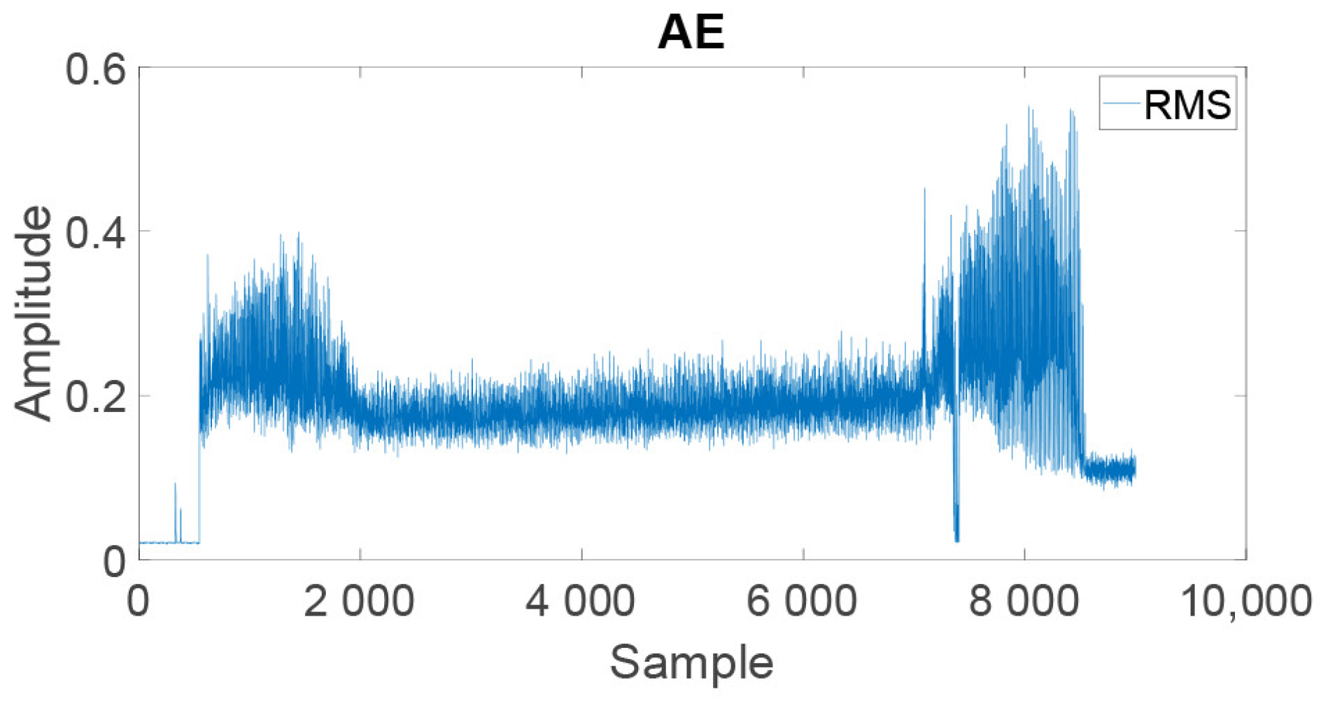
Each case has a unique number of passes in the tool on the workpiece; this variable is called run. The duration of each case is represented by the variable time. Finally, the sensor variables are the root mean square (RMS) values collected in around 9000 samples. Only two of these are used, namely the vibration signals from the variable vib_table and AE from the variable AE_table. Typical raw AE signal values are shown in Figure 1.
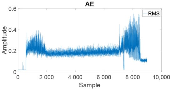
Figure 1.
Typical raw RMS values of AE sensor in a run.
Some missing values (NaN) were found in the MATLAB structure. This had already been considered, as the Readme of the dataset mentions that the VB was not measured for each run. Therefore, the samples (run) with missing values were simply removed using MATLAB’s own function. The DOC and feed variables were also removed, considering that they were redundant as the case already represents a combination of these variables.
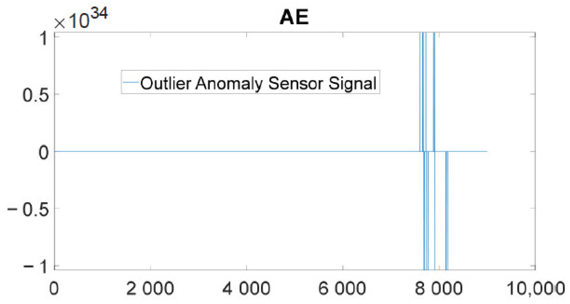
The vib_table and AE_table sensor variables were split into statistical variables, specifically the mean, variance, skewness, and kurtosis for each signal. A simple analysis of the mean values of the statistics highlighted an anomaly in the mean and variance values, leading to a huge difference between the values. The outlier sample value was highlighted (Figure 2); it appears that the signal was corrupted and, consequently, removed from all tables, resulting in much more realistic values. The statistical values replaced the signal values with 8 new variables, specifically, m_AE, m_vib, v_AE, v_vib, s_AE, s_vib, k_AE and k_vib. Each variable’s name represents a combination of the first letter of the mean, variance, skewness or kurtosis, and AE or vibration specifying the statistical value and sensor. The resulting table had 145 samples and 13 scalar variables.
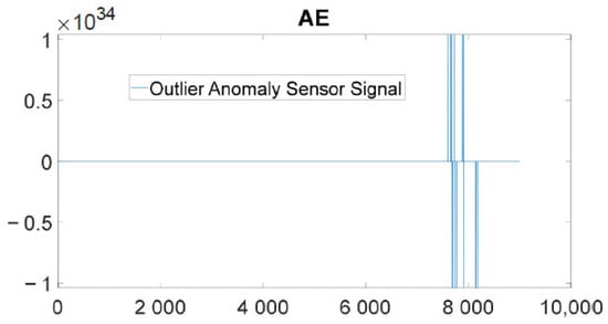
Figure 2.
Outlier anomaly AE sensor signal.
The resulting values were normalized between 0 and 1 with a MATLAB function, but the run variable range was dependent on each case; therefore, it needed to be normalized separately, as there are different numbers of runs for each case, especially after removing some samples. The run variable was added to the normalized table after that.
Samples were split into random training and test sets, using 80% for training and 20% for testing, according to the guidelines in [11]. The same author also pointed out that the minimum and maximum values of each variable must be in the training set, so these values were removed from the random selection of the test set, with the rest going into the training set.
2.1. Backpropagation Neural Network
The MLP neural network was used as a universal function approximator, as it estimates a real value between 0 and 1, according to the normalization performed previously. The candidate topologies were 3 when using only one hidden layer, respectively, with 5, 10, and 15 neurons.
The MLP networks were trained using the generalized delta rule three times for each candidate topology. The training set had 116 samples for each training with a maximum number of 1000 epochs, all of which converged for a network accuracy and a learning rate .
The final training results (T1, T2, and T3) are compiled in Table 1, based on the number of epochs, i.e., how many times the algorithm had to be presented with all the training samples until it converged, and the mean squared error (MSE).

Table 1.
Training results.
The network only converges when the absolute value of the difference between the MSE of the current and previous epoch is less than the precision. All the training sessions had good results, except for T3 in Network 2; the best results were for T2 in Network 1 and T1 in Network 3, with the lowest MSE and the lowest number of epochs, so it converged faster.
2.2. Tests
The results are based on 9 different tests for each training and topology configuration. The main metrics used are as follows: the mean absolute percentage error (MAPE) and variance ().
3. Results and Discussion
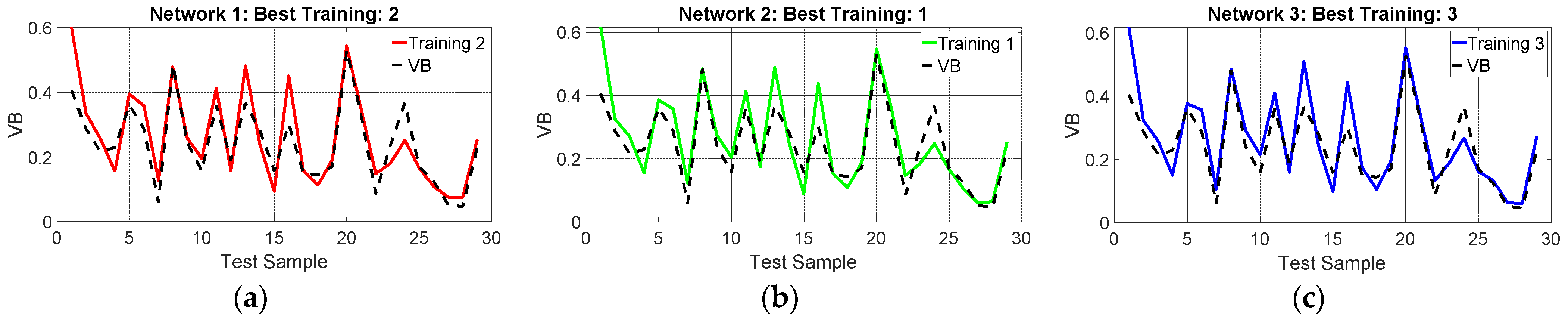
The plots in Figure 3a–c coincide with the smallest MAPE, all resulting from one of the training sessions (T1, T2, or T3) for each network compiled in Table 2. The output values are very close to the desired values, represented by a black dotted line, but there was no VB result greater than 0.5, contributing to a higher MAPE value. All the networks failed on the first sample. One solution would be to obtain more training data with high values (above 0.5) to balance the distribution, or to even have a better method for separating training and test sets, such as the k-partition cross-validation method, the aim of which would be to evaluate each network topology on different training and test subsets with a specific size (k) [11]. The best results were close to 24% MAPE and 0.43 variance in Network 3.
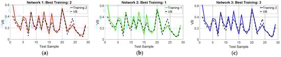
Figure 3.
Best training estimation results in (a) Network 1; (b) Network 2; (c) Network 3.
Table 2.
Test results.
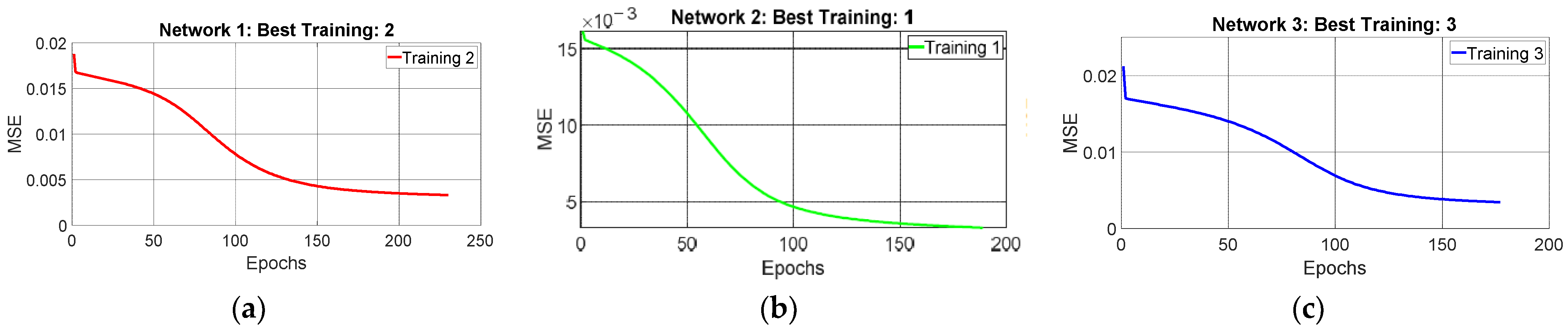
Figure 4a–c shows the convergence of each network in its best training, i.e., the MSE for each epoch. All networks had similar convergence curves, but both Networks 2 and 3 managed to converge in fewer epochs. Network 2 had the smallest MSE in the test, converging in a similar number of epochs to Network 3 in training; however, it did not perform better in the test phase.
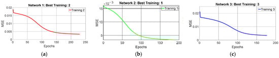
Figure 4.
Best training convergence in (a) Network 1; (b) Network 2; (c) Network 3.
4. Conclusions
This work demonstrated how a relatively simple supervised machine learning algorithm can estimate the values that come from the complex relationships between the milling tool and the workpiece. Simple methods were also used to remove features from the signal and the result was satisfactory as a proof of concept of the power of an ANN for estimating values. Clearly, more complex ANN models such as CNNs and more robust feature extraction methods such as WT would have better results, but they have higher computation costs for training compared to the MLP, which has only one layer and fast training convergences.
Still, it is possible to improve the MLP’s performance with more efficient algorithms and better data preparation, including adding two or more hidden layers and being able to reach the deep MLP (DMLP) with at least four hidden layers. Therefore, future studies should compare a more robust MLP with another more advanced ANN, considering both the accuracy and the computational cost of training and implementation. The best algorithm will be the most appropriate considering the problem constraints.
Author Contributions
Conceptualization, data curation, formal analysis, investigation, methodology, validation, writing—original draft, writing—review and editing G.O.d.S.; funding acquisition, project administration, resources, supervision, visualization, writing—review and editing, funding P.O.C.J.; formal analysis, conceptualization, methodology, resources, visualization, writing—review and editing I.N.d.S.; Data curation, methodology, resources, visualization, supervision D.B.; Conceptualization, formal analysis, software, visualization, supervision F.R.L.D. All authors have read and agreed to the published version of the manuscript.
Funding
Pro-Rectory of Research and Innovation of the University of São Paulo under grant: #22.1.09345.01.2.
Institutional Review Board Statement
Not applicable.
Informed Consent Statement
Not applicable.
Data Availability Statement
Publicly available dataset was analyzed in this study. This data can be found here: https://data.nasa.gov/Raw-Data/Milling-Wear/vjv9-9f3x/data (accessed on 1 July 2023).
Acknowledgments
The authors would like to thank the University of São Paulo (USP) and the São Paulo Research Foundation (FAPESP) for the opportunity to carry out and publish the research.
Conflicts of Interest
The authors declare no conflicts of interest.
References
- Mohanraj, T.; Yerchuru, J.; Krishnan, H.; Aravind, R.S.N.; Yameni, R. Development of Tool Condition Monitoring System in End Milling Process Using Wavelet Features and Hoelder’s Exponent with Machine Learning Algorithms. Measurement 2021, 173, 108671. [Google Scholar] [CrossRef]
- Aghazadeh, F.; Tahan, A.; Thomas, M. Tool Condition Monitoring Using Spectral Subtraction and Convolutional Neural Networks in Milling Process. Int. J. Adv. Manuf. Technol. 2018, 98, 3217–3227. [Google Scholar] [CrossRef]
- Mohanraj, T.; Shankar, S.; Rajasekar, R.; Sakthivel, N.R.; Pramanik, A. Tool Condition Monitoring Techniques in Milling Process—A Review. J. Mater. Res. Technol. 2020, 9, 1032–1042. [Google Scholar] [CrossRef]
- Kuntoğlu, M.; Aslan, A.; Pimenov, D.Y.; Usca, Ü.A.; Salur, E.; Gupta, M.K.; Mikolajczyk, T.; Giasin, K.; Kapłonek, W.; Sharma, S. A Review of Indirect Tool Condition Monitoring Systems and Decision-Making Methods in Turning: Critical Analysis and Trends. Sensors 2020, 21, 108. [Google Scholar] [CrossRef] [PubMed]
- Teti, R.; Mourtzis, D.; D’Addona, D.M.; Caggiano, A. Process Monitoring of Machining. CIRP Ann. 2022, 71, 529–552. [Google Scholar] [CrossRef]
- Iliyas Ahmad, M.; Yusof, Y.; Daud, M.E.; Latiff, K.; Abdul Kadir, A.Z.; Saif, Y. Machine Monitoring System: A Decade in Review. Int. J. Adv. Manuf. Technol. 2020, 108, 3645–3659. [Google Scholar] [CrossRef]
- Sener, B.; Serin, G.; Gudelek, M.U.; Ozbayoglu, A.M.; Unver, H.O. Intelligent Chatter Detection in Milling Using Vibration Data Features and Deep Multi-Layer Perceptron. In Proceedings of the 2020 IEEE International Conference on Big Data (Big Data), Atlanta, GA, USA, 10–13 December 2020; pp. 4759–4768. [Google Scholar]
- Huang, Z.; Zhu, J.; Lei, J.; Li, X.; Tian, F. Tool Wear Monitoring with Vibration Signals Based on Short-Time Fourier Transform and Deep Convolutional Neural Network in Milling. Math. Probl. Eng. 2021, 2021, 9976939. [Google Scholar] [CrossRef]
- Zhang, X.; Han, C.; Luo, M.; Zhang, D. Tool Wear Monitoring for Complex Part Milling Based on Deep Learning. Appl. Sci. 2020, 10, 6916. [Google Scholar] [CrossRef]
- Agogino, A.; Goebel, K. Milling Data Set; Nasa Ames Prognostics Data Repository: Moffett Field, CA, USA, 2007. [Google Scholar]
- Nunes, I.S.; Spatti, D.H.; Flauzino, R.A.; Liboni, L.H.B.; Alves, S.F.R. Artificial Neural Networks: A Practical Course; Springer: Berlin/Heidelberg, Germany, 2018. [Google Scholar]
Disclaimer/Publisher’s Note: The statements, opinions and data contained in all publications are solely those of the individual author(s) and contributor(s) and not of MDPI and/or the editor(s). MDPI and/or the editor(s) disclaim responsibility for any injury to people or property resulting from any ideas, methods, instructions or products referred to in the content. |
© 2023 by the authors. Licensee MDPI, Basel, Switzerland. This article is an open access article distributed under the terms and conditions of the Creative Commons Attribution (CC BY) license (https://creativecommons.org/licenses/by/4.0/).