Evaluation of Combined Effect of Zero Flux and Convective Boundary Conditions on Magnetohydrodynamic Boundary-Layer Flow of Nanofluid over Moving Surface Using Buongiorno’s Model ^†

Abstract

This study explores the synergistic impact of zero flux and convective boundary conditions on the magnetohydrodynamic (MHD) boundary-layer slip flow of nanofluid over a moving surface, utilizing Buongiorno’s model. In a landscape of expanding nanofluid applications, understanding boundary condition interactions is crucial. Employing a systematic approach, we varied key parameters, including surface velocity, thermophoresis, Brownian motion, Eckert number, Prandtl number, and Lewis number, systematically investigating their effects on flow and heat transfer. Numerical simulations focused on critical metrics such as skin friction coefficients; Nusselt and Sherwood numbers; and temperature, concentration, and velocity profiles. Noteworthy findings include the amplifying effect of a magnetic field and viscous dissipation on temperature profiles and the dual impact of heightened velocity slip on temperature and velocity profiles, which result in a thicker concentration boundary layer. Beyond academia, we envision our research having practical applications in optimizing high-temperature processes, bio-sensors, paints, pharmaceuticals, coatings, cosmetics, and space technology.

1. Introduction

In recent decades, the exploration of nanofluids has evolved into a dynamic field of study, driven by the pursuit of enhanced heat transfer performance. Buongiorno’s groundbreaking model in 2006 [1] has been pivotal in unraveling the intricate dynamics of nanofluids, providing a foundational framework for subsequent investigations. This literature review navigates through key studies, all grounded in Buongiorno’s model, to elucidate the multifaceted nature of nanofluid behavior and its implications across diverse applications. Buongiorno’s seminal work in 2006 laid the groundwork for nanofluid exploration, dissecting the mechanisms behind heightened thermal conductivity and heat transfer coefficients. Brownian diffusion and thermophoresis were identified as critical slip mechanisms, not only demystifying fundamental nanofluid behavior but also setting the stage for subsequent inquiries into convective heat transfer augmentation.

Extending the scope, studies such as [2], in which an investigation into natural convection over a vertical plate was carried out, illuminated the nuanced impact of Brownian motion and thermophoresis. Ref. [3], simulations within a square cavity optimized nanoparticle volume fractions for maximal heat transfer efficiency. In 2015, ref. [4] explored lid-driven cavity flow, highlighting the influence of volume fraction and nanoparticle diameter on heat transfer dynamics.

Venturing into magnetohydrodynamic realms, ref. [5] examined nanofluid behavior over a porous stretching sheet with MHD effects, contributing insights into velocity and temperature profiles, nanoparticle concentration, and local Nusselt and Sherwood numbers. The use of the Optimal Homotopy Analysis Method in [6] unveiled the complexities of MHD nanofluid flow over a stretching permeable surface. Ref. [7] explored thermal and velocity slips and delved into the nuanced effects of various parameters on nanofluid characteristics. Refs. [8,9] modified the Buongiorno nanoliquid model, offering a fresh perspective on nanofluid behavior near a stretching/shrinking sheet and expanding the applications of nanofluids in science and technology.

In recent years, studies like [10] have propelled us into the future, focusing on the mixed convective flow of a hybrid nanofluid over a heated stretching disk with zero-mass flux. Employing the modified Buongiorno model, this research delved into the impacts of mass suction and viscous dissipation, providing comprehensive insights into diverse aspects of heat and mass transfer.

This comprehensive literature review encapsulates the trajectory of nanofluid research, all anchored in the foundational insights provided by Buongiorno’s model. Each study acts as a vital building block in the collective edifice of knowledge, propelling us toward advanced thermal management and innovative engineering solutions.

The research landscape has witnessed significant endeavors to unravel the complexities of convective boundary conditions in fluid dynamics and heat transfer. Crucial for applications across industries such as thermal management systems, energy conversion technologies, and heat exchangers, understanding fluid behavior under convective conditions has been a persistent focus. Notable contributions include [9], in which early insights into the effects of convective boundary conditions on the flow and heat transfer characteristics of a stretching sheet were presented. Subsequent studies by [11,12,13] expanded our understanding by exploring convective boundary-layer flow over vertical plates and stretching sheets. Ref. [14] delved into the influence of convective conditions on mixed-convection boundary-layer flows, while [15] examined convective boundary conditions in the context of a cylinder with zero flux [16] provided insights into convective heat transfer characteristics on rotating surfaces. The research horizon extended to 2023 with [17], in which a comprehensive analysis of dusty fluid flow in a resistive porous medium under magnetohydrodynamic conditions was carried out, considering the impact of convective boundary conditions on heat transfer. This collective body of work forms the foundation for our current exploration of the combined effect of zero flux and convective boundary conditions in the MHD boundary-layer flow of nanofluids over a moving surface, aiming to contribute to the evolving understanding of fluid dynamics and heat transfer.

The study of boundary-layer flow over a moving plate has been of significant research interest in the field of fluid mechanics and thermal sciences. Several studies have investigated the behavior of fluid flow over moving surfaces, considering various influencing factors such as magnetic fields, slip conditions, viscous dissipation, radiation, chemical reactions, and nanofluids. Refs. [18,19] presented a mathematical model of boundary-layer flow over a moving plate in a nanofluid with viscous dissipation. Ref. [19] conducted a numerical simulation of boundary-layer flow over a moving plate in the presence of a magnetic field and slip conditions. Ref. [20] investigated the influence of a transverse magnetic field, viscous dissipation, and slip conditions on a steady two-dimensional incompressible laminar boundary-layer flow across a moving plate in a nanofluid. Additionally, ref. [21] unveiled the behavior of MHD mixed-convective nanofluid slip flow over a moving vertical plate with radiation, chemical reaction, and viscous dissipation, making significant contributions to future research in this area.

Despite the extensive exploration of nanofluids and convective boundary conditions, a notable research gap persists. The existing body of work has significantly advanced our understanding of nanofluid behavior, particularly under the influence of convective boundary conditions. However, a comprehensive investigation into the combined effect of zero flux and convective boundary conditions in the MHD boundary-layer flow of nanofluid over a moving surface remains limited. Existing studies have focused on specific aspects such as thermal conductivity enhancement, heat transfer coefficients, and various slip mechanisms, yet a holistic understanding of the intricate interplay between zero flux and convective conditions in the context of nanofluid dynamics is lacking.

This research aims to bridge this gap by delving into unexplored territory, offering a nuanced perspective on the combined influence of zero flux and convective boundary conditions. By employing Buongiorno’s model, this study seeks to provide a comprehensive analysis of MHD boundary-layer flow, contributing essential insights to the evolving landscape of fluid dynamics and heat transfer. The outcomes of this research endeavor aspire to fill the existing void, offering valuable contributions to the scientific community and paving the way for further advancements in the field.

2. Mathematical Formulation

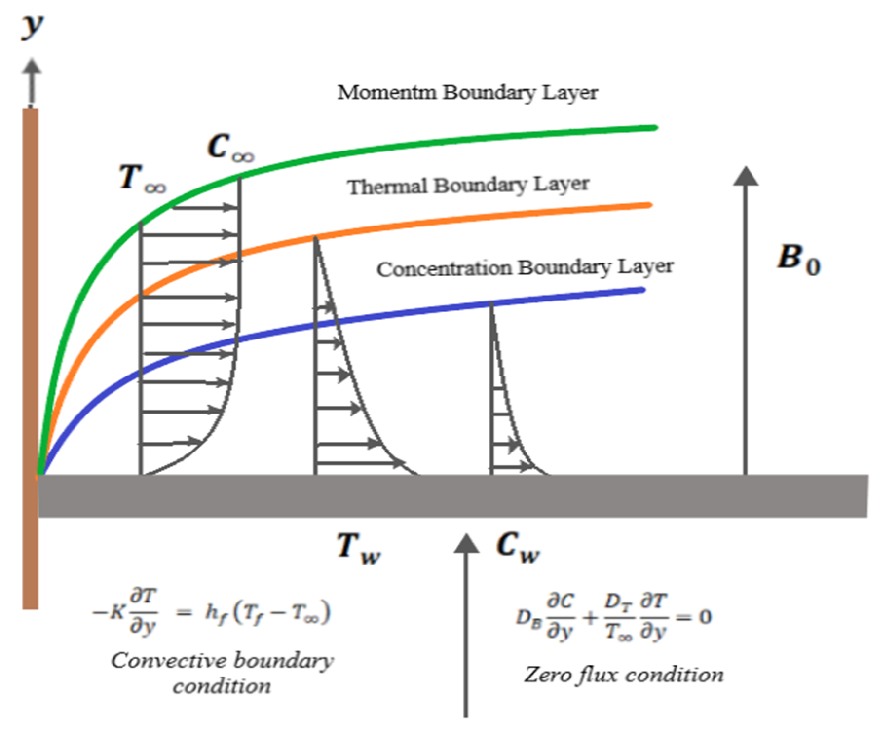
A steady two-dimensional, incompressible, laminar boundary-layer flow over a moving plate immersed in a nanofluid with the impact of a traverse magnetic field, viscous dissipation, and slip conditions is considered. It is assumed that at time $t=0$, the plate starts to move with the constant velocity $u_{w }\left(x\right)=\epsilon U_{\infty }$ in an external free stream of uniform velocity $U_{\infty }$, where $\epsilon$is a plate velocity parameter defined by Weidman [22]. The flow takes place at $y\ge 0$, where $y$ is the coordinate measured normal to the moving surface. The velocity components $u$ and $v$ are along the $x$and $y$ axis, respectively. A traverse magnetic field $B_0$ is applied in the direction of x. It is also assumed that $T$ is the temperature inside the boundary layer, $T_{\infty }$ is the ambient temperature, and $T_w$ is the wall temperature. Furthermore, $C$ is the nanoparticle volume fraction, $C_w$ is the nanoparticle volume fraction at the surface, and $C_{\infty }$ is the ambient nanoparticle volume fraction. The physical geometry of the problem is shown in Figure 1.

$$\frac{\partial u}{\partial x}+\frac{\partial v}{\partial y}=0$$

(1)

$$u\frac{\partial u}{\partial x}+v\frac{\partial u}{\partial y}=\nu \frac{{\partial }^{2}u}{\partial y^2}-\frac{\sigma B_0^2}{\rho }u$$

(2)

$$u\frac{\partial T}{\partial x}+v\frac{\partial T}{\partial y}=\frac{k}{\rho C_p}\frac{{\partial }^{2}T}{\partial y^2}+\tau \left(D_B \frac{\partial C}{\partial y}\frac{\partial T}{\partial y}+\frac{D_T}{T_{\infty }} {\left(\frac{\partial T}{\partial y}\right)}^2\right)+\frac{\mu }{\rho C_p}{\left(\frac{\partial u}{\partial y}\right)}^2$$

(3)

$$u\frac{\partial C}{\partial x}+v\frac{\partial C}{\partial y}=D_B\frac{{\partial }^{2}C}{\partial y^2}+\frac{D_{T }}{T_{\infty }}\frac{{\partial }^{2}T}{\partial y^2}$$

(4)

Subjected to the boundary conditions

$$\{\begin{array}{c}v=\epsilon V_0,\hspace{1em}u=U_{\infty },\hspace{1em}T=T_{\infty },\hspace{1em}C=C_{\infty },\hspace{1em}{D}_B\frac{\partial C}{\partial y}+\frac{D_T}{T_{\infty }}\frac{\partial T}{\partial y}=0,\hspace{1em}-K\frac{\partial T}{\partial y}=h_f(T_f-T)\hspace{1em}\mathit{at}\hspace{1em}y=0\\ u\to U_{\infty },\hspace{1em}T\to T_{\infty },\hspace{1em}C\to C_{\infty },\hspace{1em}\hspace{1em}\hspace{1em}\hspace{1em}\hspace{1em}\hspace{1em}\mathit{at}\hspace{1em}y\to \infty \end{array}$$

(5)

where $u$ and $v$ are the velocity component along the $x$ and $y$ direction, respectively, $\mu$ is the dynamic velocity, $v\left(=\frac{m}{r}\right)$ is the kinematic viscosity, $\rho$is the density of fluid, $k$ is the thermal conductivity, and $C_p$ is the specific heat capacity at constant pressure. Also, $D_B$ is the Brownian diffusion coefficient, $D_T$ is the thermophoresis diffusion coefficient, and $\mathsf{\tau }$is the ratio of the effective heat capacity of the nanoparticle material and the heat capacity of the ordinary fluid. The lower surface of the plate is heated by convection from a hot fluid at temperature $T_f$, which provides a heat transfer coefficient $h_f$.

Equation (1) is the well-known equation of continuity which signifies the principle of mass conservation, while Equation (2) represents the Navier–Stokes equation based on the law of conservation of momentum. The terms on the left-hand side (LHS) of Equation (2) are known as the advective terms, whereas the second terms on the right-hand side (RHS) are due to a magnetic field. The third term on the RHS of energy in Equation (3) adds the impact of viscous dissipation.

The set of similarity for Equations (1)–(4) subjected to the boundary conditions (5) are presented.

Similarity transformation is defined as follows:

$$\begin{gathered} \eta ={\left(\frac{U_{\infty }}{2\nu x}\right)}^{1/2}y,\psi ={\left(2U_{\infty }\nu x\right)}^{1/2}f\left(\eta \right) \\ T=T_{\infty }+\left(T_w-T_{\infty }\right)\theta \left(\eta \right) \\ C=C_{\infty }+\left(C_w-C_{\infty }\right)\varphi \left(\eta \right) \\ \theta \left(\eta \right)=\frac{T-T_{\infty }}{T_w-T_{\infty }},\varphi \left(\eta \right)=\frac{C-C_{\infty }}{C_w-C_{\infty }} \end{gathered}$$

(6)

where $\theta \mathrm{and}\varphi$ are the dimensionless temperature and resealed nanoparticle volume fraction of the fluid, respectively. The stream function $\psi \mathrm{is}\mathrm{defined}\mathrm{by}u=\frac{\partial \psi }{\partial y}$ and $v=-\frac{\partial \psi }{\partial x}$, so that Equation (1) is satisfied identically, which results in

$$u=U_{\infty }{f}^{\prime }\left(\eta \right)$$

(7)

$$v=-{\left(\frac{U_{\infty }\nu }{2x}\right)}^{\frac{1}{2}}f\left(\eta \right)+\frac{U_{\infty }y}{2x}{f}^{\prime }\left(\eta \right)$$

(8)

By applying the similarity transforms on the remaining governing Equations (2)–(5), the similarity equations are obtained as follows:

$$f^{‴}+f{f}^{″}-M{f}^{\prime }=0$$

(9)

$$\frac{1}{P_r}{\theta }^{″}+f{\theta }^{\prime }+N_b{\theta }^{\prime }{\varphi }^{\prime }+N_t{\theta }^{\prime 2}+Ec{f}^{″2}=0$$

(10)

$${\varphi }^{″}+\frac{N_t}{N_b}{\theta }^{″}+Lef{\varphi }^{\prime }=0$$

(11)

where $Pr=\frac{v\rho C_p}{k}$ is the Prandtl number, $N_b=\frac{\tau D_B\left(C_{w }-C_{\infty }\right)}{v}$ is the Brownian motion parameter, $N_t=\frac{\tau D_T\left(T_{w }-T_{\infty }\right)}{T_{\infty }v}$ is the thermophoresis parameter, $Ec=\frac{{\left(U_{\infty }\right)}^2}{C_p\left(T_w-T_{\infty }\right)}$ is the Eckert number and $Le=\frac{v}{D_B}$ is the Lewis number, $M=\frac{2x\sigma B_0^2}{\rho U_{\infty }}$ is the magnetic parameter, and $h_f=\frac{c}{\sqrt{x} }$, where c is the constant.

The corresponding boundary conditions are as follows:

$$\{\begin{array}{c}f(\eta )=\epsilon V_0,f^{\prime }(\eta )=0,{\theta }^{\prime }(\eta )=-{\beta }_i(1-\theta (\eta )),\\ N_b{\varphi }^{\prime }(\eta )+N_t{\theta }^{\prime }(\eta )=0,\hspace{1em}\hspace{1em}\mathit{at}\eta =0\\ f^{\prime }(\infty )\to 1,\hspace{1em}\theta (\infty )\to 0,\hspace{1em}\varphi (\infty )\to 0,\hspace{1em}\mathit{at}\eta \to \infty \end{array}$$

(12)

Note that ${\beta }_i=\frac{c}{k}\sqrt{\frac{v}{U}}$ is the Biot number. The physical quantities of interest, the skin friction coefficient $C_f$, the local Nusselt number $N{u}_x$, and the local Sherwood number ${\mathit{Sh}}_x$, are given by

$$C_f=\frac{{\tau }_w}{\rho u_e^2},N{u}_x=\frac{x{q}_w}{k\left(T_w-T_{\infty }\right)},S{h}_x=\frac{x{j}_w}{D_B\left(C_w-C_{\infty }\right)}.$$

(13)

The surface shear stress ${\mathsf{\tau }}_w$, the surface heat flux $q_w$, and the surface mass flux $j_w$ are given by

$${\tau }_w=\mu {\left(\frac{\partial u}{\partial y}\right)}_{y=0},q_w=-k{\left(\frac{\partial T}{\partial y}\right)}_{y=0},j_w=-D_B{\left(\frac{\partial C}{\partial y}\right)}_{y=0}$$

(14)

with µ = ρv being the dynamic viscosity. Using the similarity variables in Equation (6), the following relations are obtained:

$$C_f{\left(2R{e}_x\right)}^{1/2}=f^{″}\left(0\right),N{u}_x{\left(\frac{R{e}_x}{2}\right)}^{-1/2}=-{\theta }^{\prime }\left(0\right),S{h}_x{\left(\frac{R{e}_x}{2}\right)}^{-1/2}=-{\varnothing }^{\prime }\left(0\right)$$

(15)

where $R{e}_x=\frac{U_{\infty }x}{v}$ is the local Reynolds number and ${\left(2R{e}_x\right)}^{1/2},N{u}_x{\left(\frac{R{e}_x}{2}\right)}^{-\frac{1}{2}},\mathrm{and}S{h}_x{\left(\frac{R{e}_x}{2}\right)}^{-1/2}$ are referred to as the reduced skin friction coefficient, the reduced Nusselt number, and the reduced Sherwood number and can be denoted as $C_{fr},$ Nur, and Shr, which are represented by $f^{″}\left(0\right),-{\theta }^{\prime }\left(0\right),\mathrm{and}-{\varnothing }^{\prime }\left(0\right),$ respectively.

3. Method of Solution

To solve Equations (9)–(11) along with the boundary conditions (12), we will transform the third-order derivative into a second-order derivative by replacing $f^{\prime }=F$.

Then, the above system of equations will become

$$f^{\prime }=F$$

(16)

$$F^{″}+f{F}^{\prime }-MF=0$$

(17)

$${\theta }^{″}+P_{r}f{\theta }^{\prime }+P_r{N}_b{\theta }^{\prime }{\varphi }^{\prime }+P_r{N}_t{\theta }^{\prime 2}+P_{r}Ec{F}^{\prime 2}=0$$

(18)

$${\varphi }^{″}+\frac{N_t}{N_b}{\theta }^{″}+L_{e}f{\varphi }^{\prime }=0$$

(19)

The corresponding boundary conditions will be transformed to

$$\{\begin{array}{c}f(\eta )=V_0,F(\eta )=c+F^{\prime }(\eta ),\hspace{1em}\theta (\eta )=\lambda {\theta }^{\prime }(\eta ),\hspace{1em}\varphi (\eta )=\lambda {\varphi }^{\prime }(\eta ),\hspace{1em}\hspace{1em}\mathit{at}\eta =0\\ F(\eta )\to 1,\theta (\eta )\to 0,\hspace{1em}\varphi (\eta )\to 0,\hspace{1em}\hspace{1em}\mathit{at}\hspace{1em}\eta \to \infty \end{array}$$

(20)

System (16) to (19) is a nonlinear one. To obtain the solution of this system, it is firstly required to convert these equations into a system of linear differential equations. This is performed by the Newton linearization method, which is mentioned in the following sections.

4. Linearization of Equations

Equation (16) is linear in variable $f$; therefore, it is not necessary to make it linear. We will make Equation (16) linear in variable $F$ while taking all other variables as constants. The same will be done for Equation (18). Equation (19), however, is linear in variable $\varphi$.

Equation (17) is written as follows:

$$F^{″}=-f{F}^{\prime }+MF$$

Defining the right hand side as $h_F\left(\eta ,F,F^{\prime }\right)$, it is defined as follows:

$$h_F\left(\eta ,F,F^{\prime }\right)=-f{F}^{\prime }+MF$$

Now,

$${\left(A_F\right)}_n=-{\left(\frac{\partial h_F}{\partial F^{\prime }}\right)}_n=-\left[-f_n\right]=f_n$$

$n$ in the above equation represents the solution at the previous iteration; $A_n$ from the above equation will become

$${\left(A_F\right)}_n=f_n$$

$${\left(B_F\right)}_n=-{\left(\frac{\partial h_F}{\partial F}\right)}_n=-\left[M\right]=-M$$

$${\left(B_F\right)}_n=-M$$

$${\left(D_F\right)}_n=h_F\left(\eta ,F_n,F_n^{\prime }\right)-{\left(\frac{\partial h_F}{\partial F} \right)}_n F_n-{\left(\frac{\partial h_F}{\partial F_n^{\prime }} \right)}_n{F}_n^{\prime }$$

$${\left(D_F\right)}_n=h_F\left(\eta ,F_n,F_n^{\prime }\right)+{\left(B_F\right)}_n F_n+{\left(A_F\right)}_n{F}_n^{\prime }$$

Hence, the linearized equation in variable $F$ is given as

$$F_{n+1}^{″}+A_n{F}_{n+1}^{\prime }+B_n{F}_{n+1}=h_F\left(\eta ,F_n,F_n^{\prime }\right)+{\left(B_F\right)}_n F_n+{\left(A_F\right)}_n{F}_n^{\prime }$$

(21)

$$F_{n+1}^{″}+{\left(A_F\right)}_n F_{n+1}^{\prime }+{\left(B_F\right)}_n F_{n+1}={\left(D_F\right)}_n$$

(22)

Similarly, Equations (18) and (19) are now linear and will be iteratively solved as linear second-order differential equations. Thus, the system of equations to be solved is as follows:

$$\{\begin{array}{l}{f}^{\prime }=F\\ F_{n+1}^{″}+{\left(A_F\right)}_n{F}_{n+1}^{\prime }+{\left(B_F\right)}_n{F}_{n+1}={\left(D_F\right)}_n\\ {\theta }_{n+1}^{″}+{\left(A_{\theta }\right)}_n{\theta }_{n+1}^{\prime }+{\left(B_{\theta }\right)}_n{\theta }_{n+1}={\left(D_{\theta }\right)}_n\\ {\varphi }^{″}+\frac{N_t}{N_b}{\theta }^{″}+L_{e}f{\varphi }^{\prime }=0\end{array}$$

(23)

Along with the following boundary conditions:

$$\{\begin{array}{c}f=V_0, F\left(\eta \right)=c+F^{\prime }\left(\eta \right), \theta \left(\eta \right)=\lambda {\theta }^{\prime }\left(\eta \right), \varphi \left(\eta \right)=\lambda {\varphi }^{\prime }\left(\eta \right), at \eta =0\\ F\to 0, \theta \to 0, \varphi \to 0, at \eta \to \infty \end{array}$$

(24)

The system of four linear equations in (23) is solved using the Finite Element Method in MATLAB. Each equation undergoes discretization, numerical differentiation for coefficient evaluation, and reformulation into a weak form. MATLAB is then employed to solve the system, accounting for Dirichlet boundary conditions. This process is repeated for the second, third, and fourth equations, with the first equation being directly integrated in the weak form for a separate solution.

5. Results and Discussion

In our comprehensive exploration of nanofluid behavior in boundary-layer flow over a stretching surface, we scrutinize six pivotal parameters: Prandtl number $(P_r)$, plate velocity parameter $\left(ϵ\right)$, Brownian motion parameter $(N_b)$, thermophoresis parameter$(N_t)$, Eckert number $\left(Ec\right)$, and Lewis number$\left(Le\right)$. These parameters, consistent with the established literature [18,19,20,21,22], form the basis of our analysis.

Understanding the interplay between these parameters is crucial. Figure 2 unveils the temperature profiles, θ(η), under varying $N_t$ conditions. As $N_t$ escalates, a discernible upward trend emerges in the temperature profile. Physically, this aligns with the heightened Brownian motion of the nanoparticles, resulting in an expanded thermal boundary-layer thickness and an elevated overall temperature, as corroborated by the increased nanoparticle volume fraction. This trend continues in Figure 3, where concentration profiles ∅(η) under various $N_t$ conditions exhibit a notable decline with increasing $N_t$. The heightened Brownian motion expands the thermal boundary layer, influencing the concentration of nanoparticles near the surface through the stronger impact of thermophoresis.

.

.

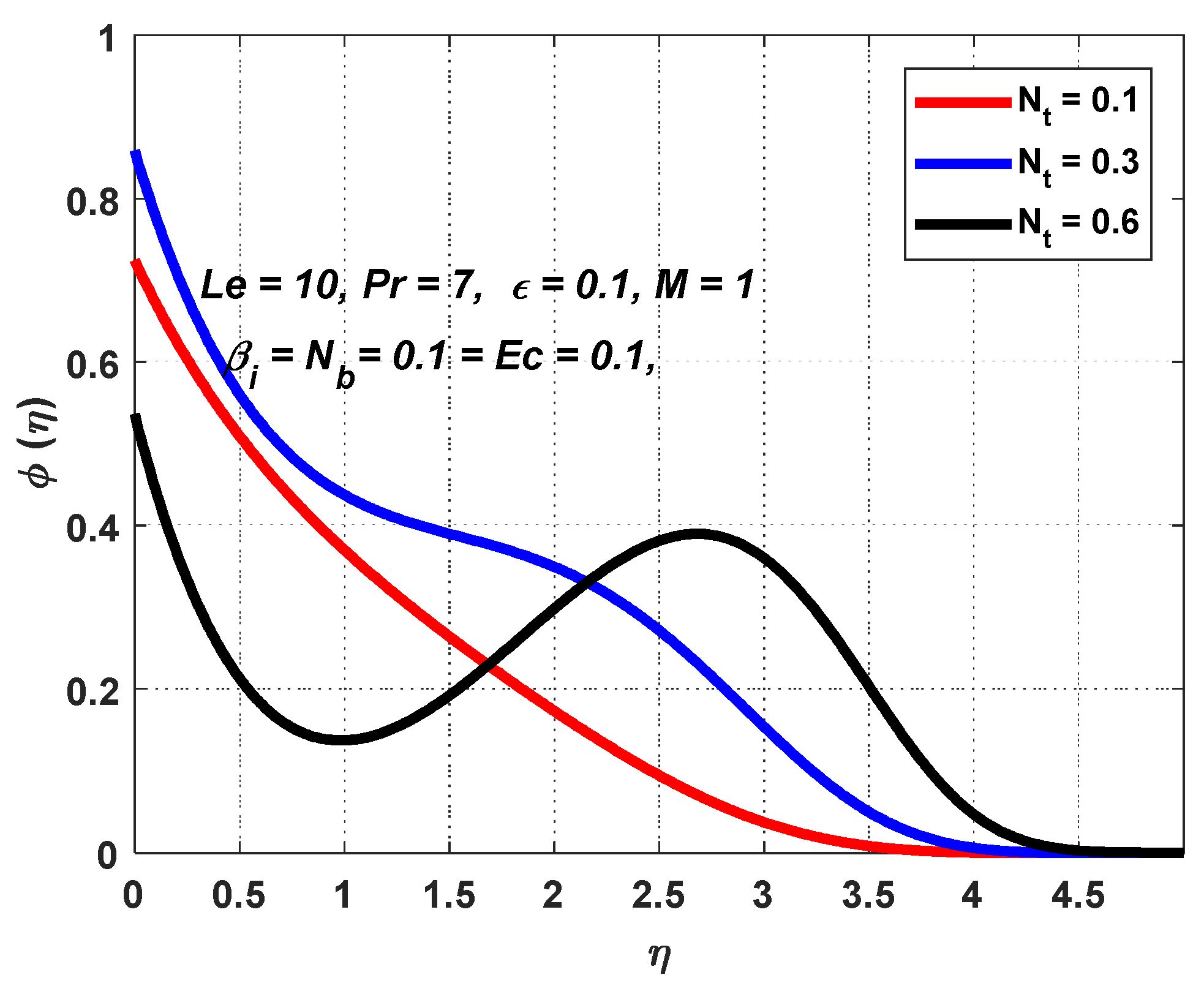
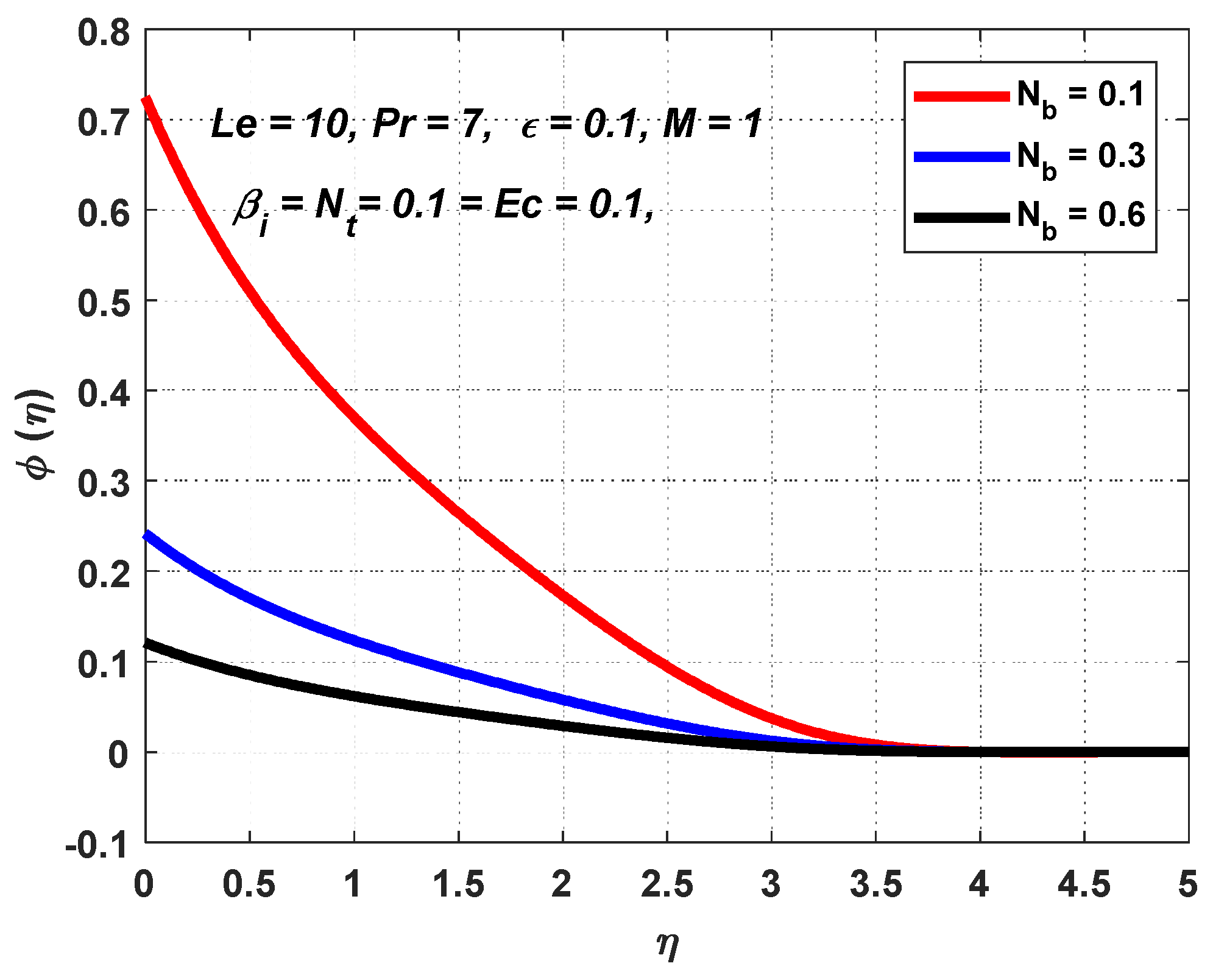
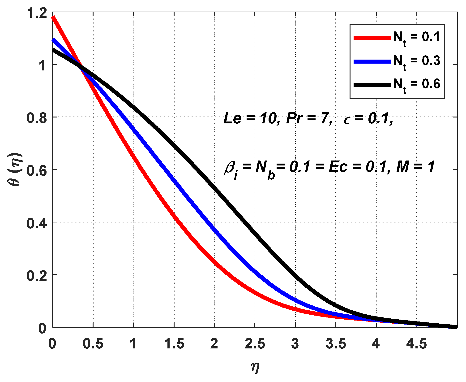
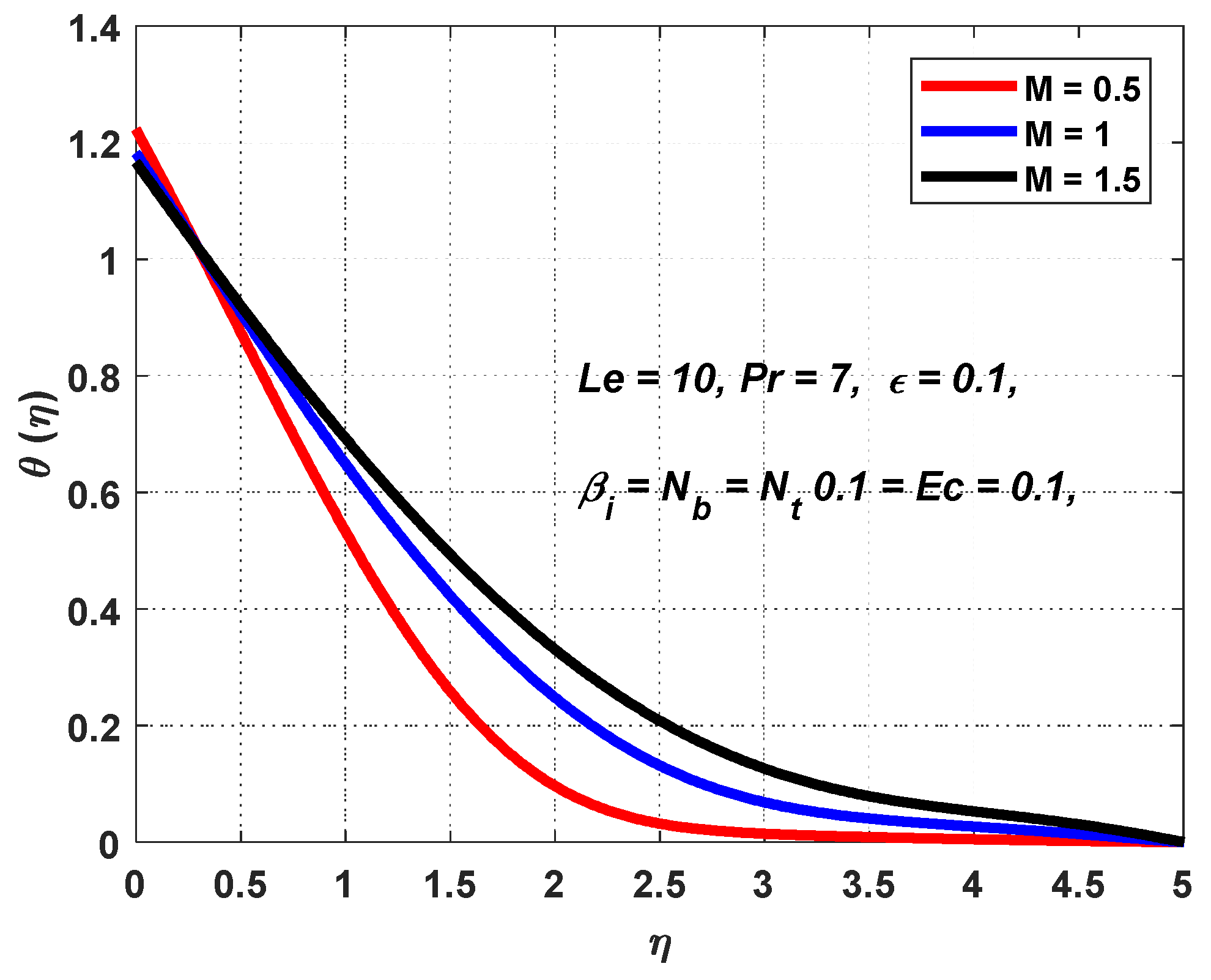
Expanding our understanding, Figure 4 delves into concentration profiles, ϕ(η), for varying $N_b$ values. As $N_b$ increases, the concentration near the surface decreases due to enhanced Brownian motion, aligning seamlessly with prior studies on $N_b$’s influence on nanofluid concentration profiles. Figure 5 introduces magnetic field strength (M) into the discussion. As M increases, temperature profiles, θ(η), rise, indicating an expanded thermal boundary layer and intensified heat transfer. This effect is attributed to the heightened magnetic field, influencing the Lorentz force, fluid velocity, and heat transfer coefficient.

.

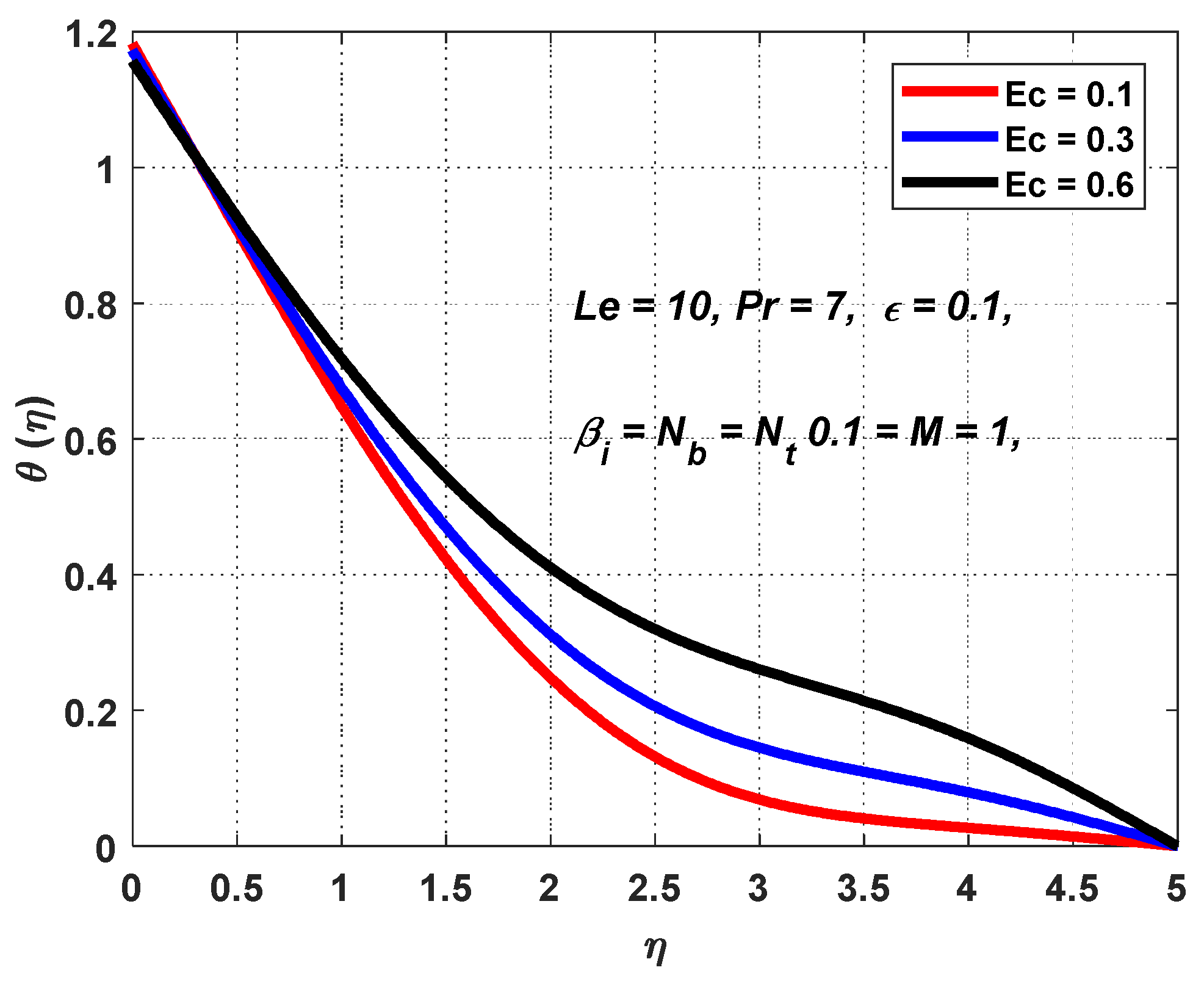
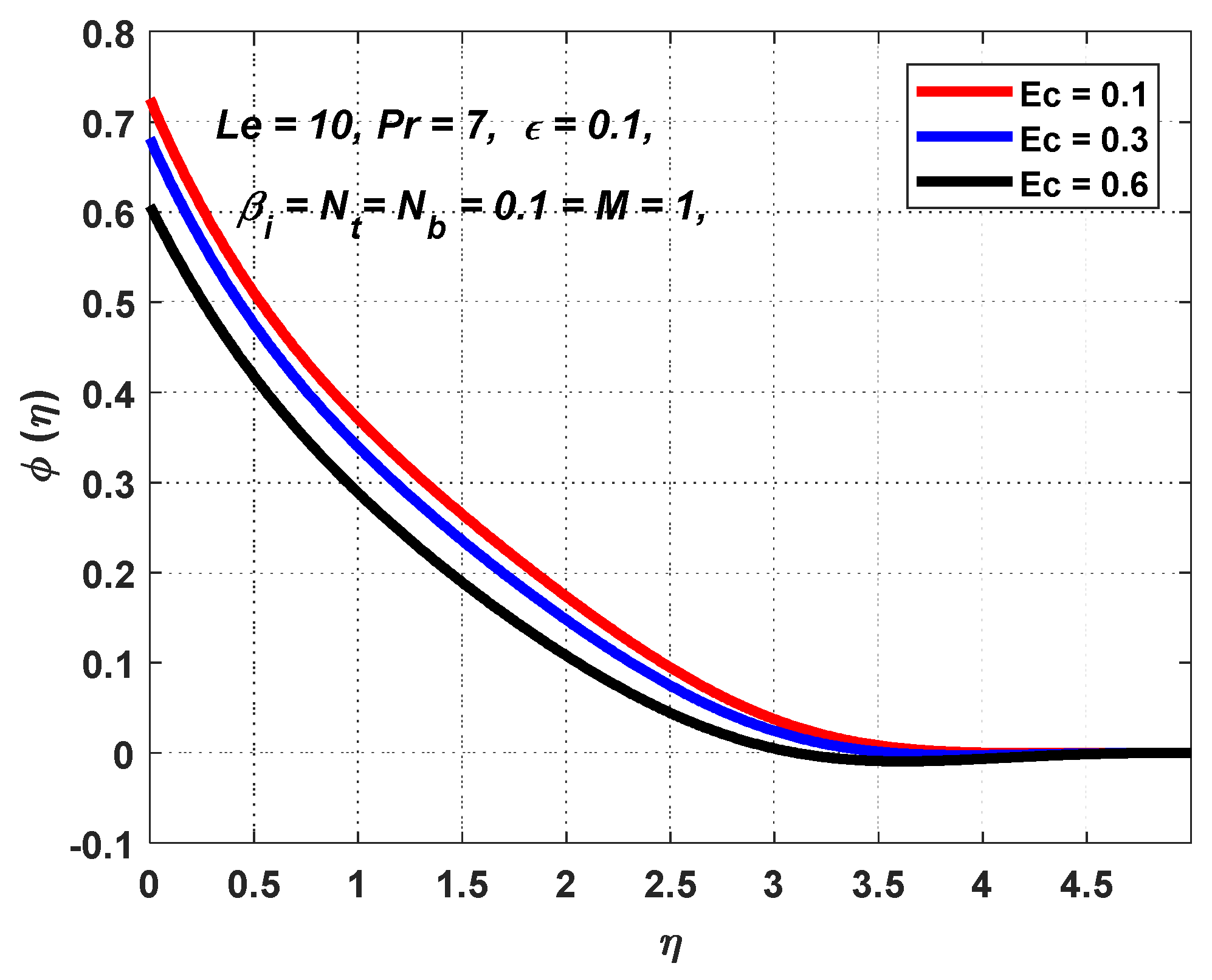
In Figure 6, temperature profiles, θ(η), vary with different Eckert numbers (Ec). Elevated Ec leads to increased temperature profiles, pointing to an expanded thermal boundary layer and heightened heat transfer. This aligns with the expected rise in fluid kinetic energy, influencing the heat transfer coefficient and resulting in an increased temperature. Shifting our focus to the concentration profiles in Figure 7 under varying Eckert numbers Ec, we observe a decrease as Ec increases. This reveals reduced nanoparticle density near the surface due to intensified Brownian motion and heightened kinetic energy, aligning with previous studies on Ec’s impact on nanofluid concentration profiles.

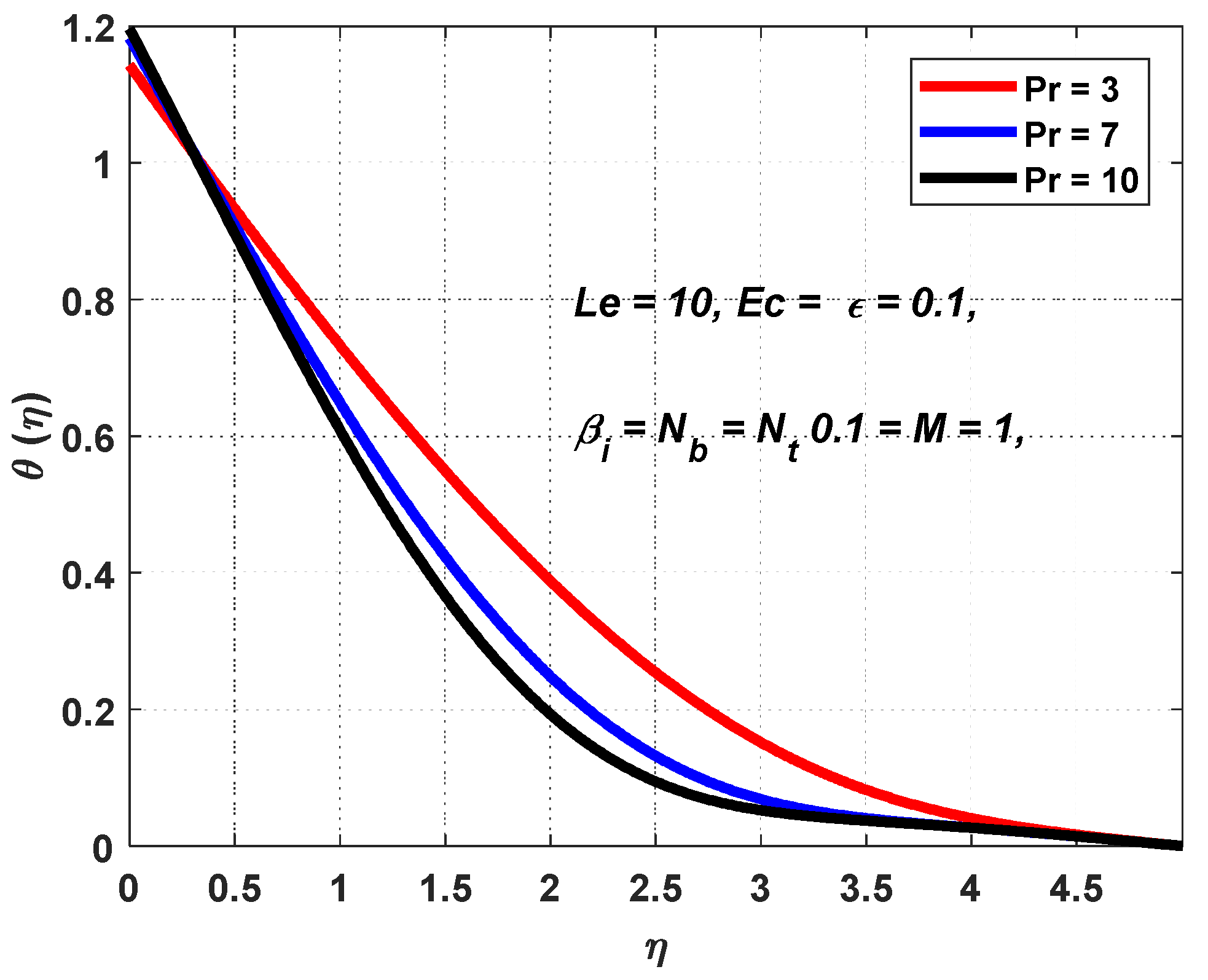
In Figure 8, temperature profiles, θ(η), at different Prandtl numbers $P_r$ are explored. As $P_r$ increases, the temperature profile decreases, indicating a reduction in thermal boundary-layer thickness due to diminished heat transfer. Elevated $P_r$ results in heightened fluid viscosity, limiting heat transfer capability and consequently lowering the temperature.

Figure 9 illustrates temperature profiles, θ(η), under varying values of the moving plate parameter ($ϵ$). An increase in $ϵ$ correlates with a decrease in temperature profiles, indicative of a thinner thermal boundary layer resulting from reduced heat transfer between the surface and the fluid. Elevated $ϵ$ leads to greater plate velocity, reducing the fluid residence time near the surface and subsequently lowering the temperature. 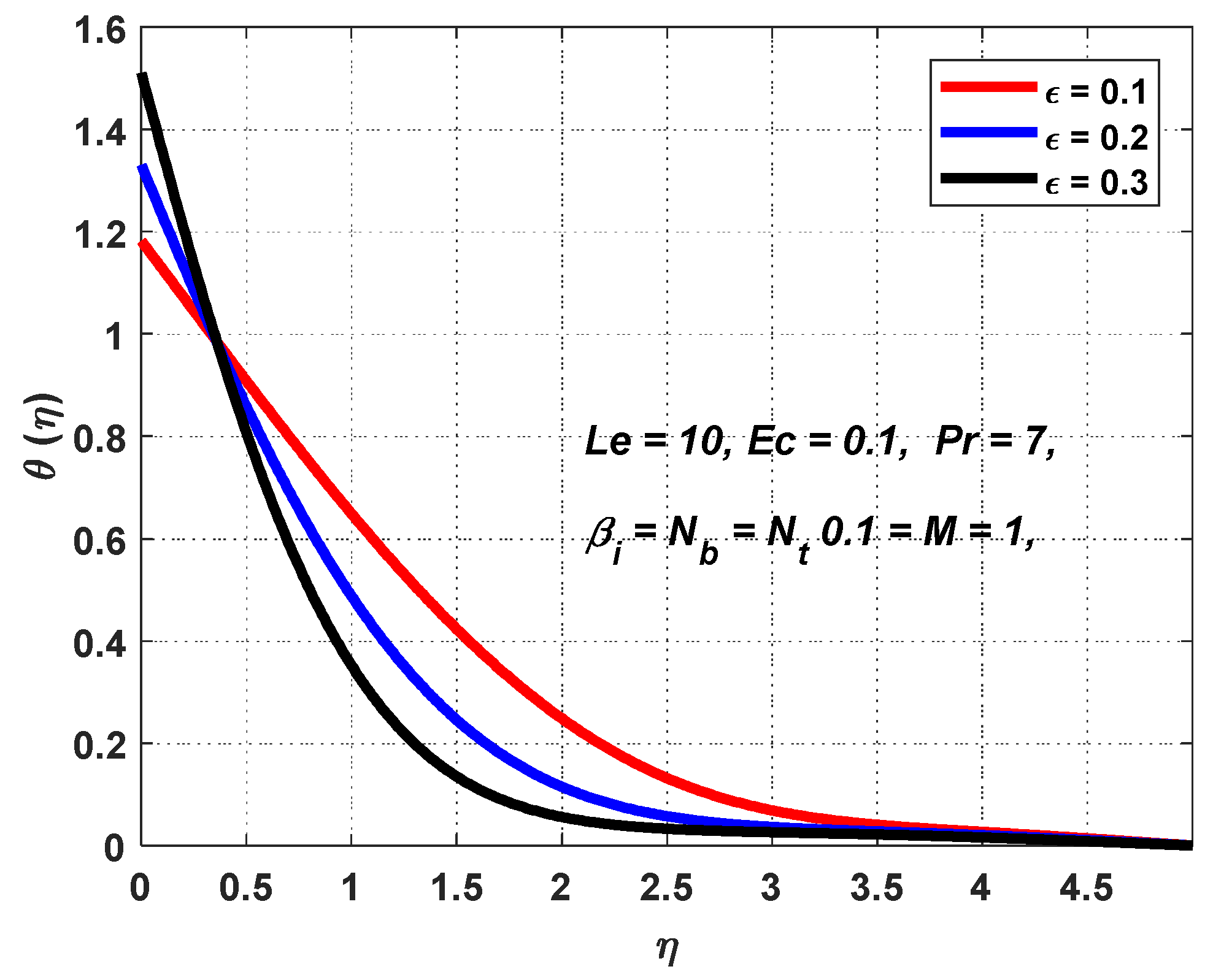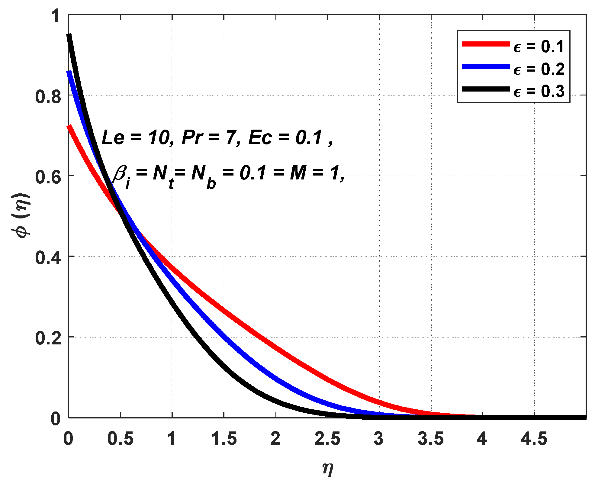Figure 10, depicting the concentration profile, ϕ(η), with different values of $ϵ$, illustrates that as the $ϵ$increases, the concentration profile (ϕ) decreases. This indicates that higher plate velocities lead to improved fluid convection, enhancing the removal of nanoparticles from the surface vicinity. Consequently, the concentration of nanoparticles near the surface decreases, aligning with expected fluid dynamics behavior, where elevated flow velocities result in reduced concentrations of suspended particles near the surface.

.

.

The observed trends collectively highlight the intricate interplay between Brownian motion, thermophoresis, magnetic fields, fluid kinetic energy, and plate velocity. These findings not only consolidate existing knowledge but also pave the way for future advancements in optimizing nanofluid applications, particularly in thermal management systems, energy conversion technologies, and heat exchangers.

6. Conclusions

In this comprehensive analysis of nanofluid behavior in boundary-layer flow over a stretching surface, the examination of key parameters provides valuable insights, shedding light on the complex interplay between these factors and their influence on thermal and concentration profiles. The nuanced understanding contributes significantly to optimizing the design of heat transfer systems and enhancing the efficiency of energy conversion technologies.

In the context of our research topic, which focuses on the combined effect of zero flux and convective boundary conditions on the MHD boundary-layer flow of nanofluid over a moving surface using Buongiorno’s model, the observed interplays present crucial insights. The specifics are as follows:

• The Prandtl number (Pr) demonstrates a clear inverse relationship with temperature profiles, emphasizing the role of fluid viscosity in heat transfer.
• The plate velocity parameter (ε) reveals that higher plate velocities lead to thinner thermal boundary layers, impacting heat transfer efficiency.
• The Brownian motion parameter ($(N_b)$ findings showcase a decrease in concentration near the surface with increasing $(N_b)$, indicating enhanced Brownian motion effects on nanoparticle diffusion.
• The thermophoresis parameter $(N_t)$ highlights an upward trend in temperature profiles, showcasing the impact of heightened Brownian motion and expanded thermal boundary layers.
• The Eckert number (Ec) demonstrates increased temperature profiles with elevated values, emphasizing the role of fluid kinetic energy in heat transfer.
• The Lewis number (Le) is not explicitly addressed in the provided text. If specific findings are available, they can be included in the comprehensive analysis.

These collective findings underscore the intricate relationships governing nanofluid behavior. The comprehensive understanding lays a foundation for future advancements in thermal management systems, energy conversion technologies, and heat exchangers, driven by the interconnected nature of these parameters. Further exploration and research are imperative to unlock the full potential of nanofluids in various engineering applications, reinforcing the significance of our study’s outcomes.