Abstract
In science and technology, the application of mathematics and mathematical modelling is crucial. A more conceptual and axiomatic approach has been taken in developing the narrative from geometry in the enormous history of mathematics. Mathematics is distinct from all other topics due to its use of theorems, proofs, axioms, corollaries, examples, results, and analysis. Applications of mathematics can be found, among others, in management sciences, biosciences, chemical technology, computer sciences, information technology, and the medical industry. Differentiation and its extensions are among the most frequently used branches in mathematics. Different curves are created when a plane connects with the surface of a cone. They are called conic sections. Conic sections have uses in physics and architecture, among other fields. In this study, differential equations are used to determine the conic section’s type and locate its center. The effectiveness of conventional and innovative teaching strategies is compared using Bayesian inference. The Bayesian method is employed to update the prior assumptions regarding the relative efficacy of the two approaches. Data on student performance in four different types of classes are gathered for the analysis.
1. Introduction
The advancement of science and technology is significantly supported by the application of mathematics. The mathematical model is the most widely used and regarded as the best among the numerous models offered for the reliability of methods and the efficiency of a given methodology. Even though theory experiments might support a problem’s methods, only mathematical development and representation of those methods are recognized as the best model. Numerous fields use mathematics in some capacity [1,2]. Numerous mathematical modelling strategies can be used to represent research problems due to the diversity of the mathematics field [3,4]. The ideas of limits and continuity are the foundational elements of differentiation. Physically, differentiation is referred to as the rate of change. The best illustration of this is given by acceleration and velocity; the time parameter is brought up in reference to both. Limits and continuity served as the foundation for differentiation; later, several approaches to identifying derivative rules were created. Then, equations involving the ideas of partial derivatives, total derivatives, derivatives of explicit functions, and so on, were established. Differential and partial differential equations are terms used to describe equations with partial derivatives. Differential and partial differential equations were created, and solutions to those equations were established.
Application of mathematical models can be found in RT-PCR [5], usability problems [6], constraint problems [7], microspheres [8], neural networks [9], estimation of flood loss [10], road cycling power [11], plant nutrition [12], product allocation and warehousing [13], hear structure [14], chemotherapy [15], bacterial growth and inactivation [16,17], malaria sensitivity analysis [18], and caspase function [19]. Various research problems are represented and analyzed using differential equations, like analyses on HIV infection [20], tumor growth [21], cancer prediction [22], forest stand [23], and the spread of disease [24]; these equations are also involved in studies of bio models using delay equations [25], virus infection [26], psychological regulations [27], toxic substances [28], flood risk [29], environment development [30], harvesting [31], and biological systems [32].
Differential equations (DE) and partial differential equations (PDE) have been applied in many fields. In physical science and chemical engineering, rates of change are modeled using differential equations and partial differential equations. This model’s ability to be solved analytically or numerically is one of its main advantages. The same can be used to model voltage and current systems in electrical and electronic technology. The solution of the modified models is ascertained by means of transforming procedures. A mathematical equation with unknown function derivatives is known as a differential equation. It describes the temporal or spatial evolution of a quantity or system. We can represent and comprehend dynamic processes in many disciplines, including physics, engineering, and economics, by solving differential equations. A differential equation with partial derivatives for several independent variables is known as a partial differential equation (PDE). PDEs investigate multidimensional phenomena like fluid dynamics, wave propagation, and heat diffusion. PDE solutions are difficult to solve, and frequently need sophisticated mathematical methods [33,34].
To locate the center and determine the type of conic section, differential and partial differential equations are applied in this study. Bayesian inference is used to compare the efficacy of various teaching strategies for various student types. An educator may have previously held the opinion that those students with a particular learning type benefit more from the standard teaching approach. The posterior distribution will, however, be more likely to favor the new strategy if the study’s data demonstrate that it is more beneficial for these learners.
2. Conic Section and Pedagogical Approach
In addition to being an essential component of mathematics, conic sections are widely used in a variety of real-world contexts, including physics, engineering, astronomy, and architecture. Their unique characteristics and forms make them great tools for understanding and addressing problems in the real world. A plane and a double-napped cone can cross to form a conic section, which is a geometric shape. Conic sections have special properties that make them interesting study subjects. Introducing novel teaching techniques into the classroom is a creative strategy. Its purpose is to make arithmetic ideas easier for children to understand, and to tackle the problem of motivating and engaging today’s tech-savvy students. The approaches and methods used by educators to impart knowledge and promote student learning are referred to as teaching methods. Engaging students, encouraging critical thinking, and ensuring improved information retention all depend on effective teaching techniques [35,36]. Different teaching techniques, including lectures, discussions, group projects, practical experiments, and multimedia presentations, accommodate various learning preferences and support the development of an engaging and welcoming learning environment. The topic at hand, student makeup, and targeted learning outcomes should all be taken into consideration when selecting a teaching strategy. To increase their efficiency in the classroom, teachers must constantly develop and be flexible [37,38].
Introducing new teaching methods could help students become much better at solving problems. It may make mathematics easier to understand and make tech-savvy students more interested in the subject. This may improve their critical thinking and make them adept at using what they have learned to solve all sorts of real-life problems. Innovative teaching methods aim to make mathematics more accessible, enjoyable, and relatable for students, ultimately improving their mathematics skills and confidence in the subject. Mathematics helps students become great at handling challenges in their studies and in real life, giving them skills they can use forever.
3. Methodology-1
It is known that the differentiation of a curve with respect to x gives the slopes of tangent that can be drawn at that point. Let us consider a few examples, as follows.
Illustration 1
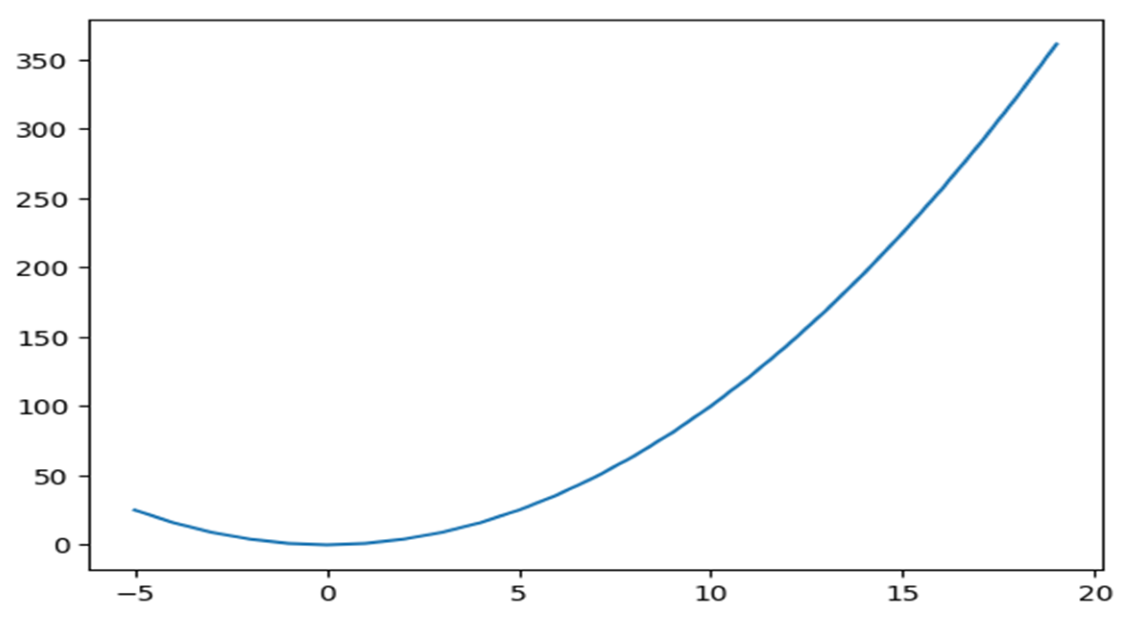
Let the curve be a parabola y = x2, as shown in Figure 1. Then, y’(x) = 2x; The point must now be substituted in the dy/dx equation in order to determine the slope of the tangent drawn at (1, 1). The slope will therefore be 2.
Figure 1.
Curve representing y = x2.
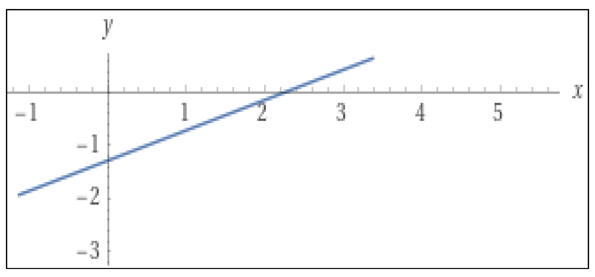
Let the curve be a straight line 4x − 7y = 9, as shown in Figure 2. Here, dy/dx = 4/7. This can be achieved straight away, since it is an equation of a straight line. From 4x − 7y = 9, y = (−4/−7) x + (9/−7); therefore, the slope is 4/7. In general, the slope of ax + by = c will be – a/b.

Figure 2.
Curve representing 4x − 7y = 9.
Let the curve be x3 + y3 + 3 × 2y + 3xy2 + x + y + 9 = 0, as shown in Figure 3. When dividing by x, dy/dx equals − (3x2 + 6xy + 3y2 + 1)/(3y2 + 3x2 + 6xy +1). By replacing the point in the dy/dx equation, we can now obtain the slope of the tangent drawn at the point (1, 1), which is −1.
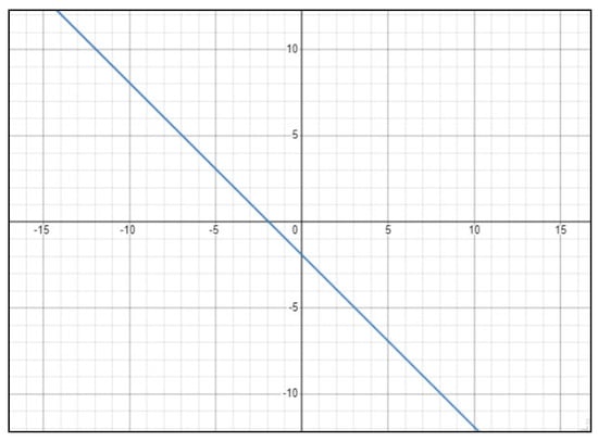
Figure 3.
Curve representing x3 + y3 + 3x2y + 3xy2 + x + y + 9 = 0.
4. Methodology-2
Partial differentiation is a field of mathematics wherein we can find the slope of a particular tangent from the set of all the tangents that can be drawn. Now, we will extend this concept of partial differentiation to finding the centers of conic sections. To be able to do this, we must follow some steps. When considering any given equation,
- Find ∂/∂x, ∂/∂y;
- Equate both to zero;
- This will give two first-order linear equations;
- These equations can be solved to obtain the required point.
Illustration 2
- (i)
- In view of a pair of straight lines, ax2 + by2 + 2hxy + 2gx + 2fy + c = 0. In the case where in h2-ab is not equal to zero, ∂/∂x = 2ax + 2hy + 2g = 0; ∂/∂y = 2by + 2hx + 2f = 0; Now, we solve x = (bg − hf)/h2 − ab, and y = (af − hg)/h2 − ab. This represents that the two straight lines converges.
- (ii)
- Considering the ellipse, (x − h)2/a2 + (y − k)2 /b2 = 1. Now, ∂/∂x = 2x − 2h = 0 implies x = h; similarly, y = k; This is the center of the ellipse. The result will be the same for the hyperbola.
- (iii)
- Now let us consider a parabola. The general equation is (y − k)2 = 4a(x − h). Now, ∂/∂y = 0, which implies y = k and x = k; this is the vertex of the parabola.
- (iv)
- Consider the Equation 5x2 + 6y2 +6x + 4y + 2 = 0. Now, Ә/Әx = 10x + 6 = 0, which implies x = −3/5; similarly, Ә/Әy = 12y + 4 = 0, which implies y = −1/3. So, the center is (−3/5, −1/3)
Now, we may find out which type of conic section the new approach is.
- i.
- Hyperbola: if the coefficient of x2 is greater than the coefficient of y2.
- ii.
- Find the eccentricity of the hyperbola by taking the x2 coefficient as b2 and the y2 coefficient as a2, and substituting in the formula b2 = a2 (e2 − 1).
- iii.
- Circle: If the coefficient of x2 is equal to coefficient of y2.
- iv.
- Parabola: If there is only one square term, that is either x2 or y2,and its eccentricity is 1.
- v.
- A pair of straightlines: If there is a xy term in the equation.
5. Bayesian Inference
Using Bayesian Inference and Bayesian Analysis, we update our beliefs and understanding of a scenario or model when new facts become available. The method is named after Thomas Bayes, a mathematician and philosopher from the 18th century. Starting with basic views about the uncertainty of a parameter or a model, probability distributions are used to express these beliefs in Bayesian inference. The posterior distribution is the result of combining new information about the parameter with prior beliefs to reach those updated beliefs. After considering the new data, the posterior distribution represents the current knowledge regarding the parameter or model. Using Bayes’ theorem, which establishes a mathematical relationship between the posterior distribution, the likelihood of observing the data, given the parameter and the prior distribution, is the fundamental concept of Bayesian inference. This is one way to express Bayes’ theorem:
where
P (Factor | Data) = P (Data | Factor) P (Factor)/P (Data)
P (Factor | Data) is the posterior distribution, representing our updated beliefs after observing the data.
P (Data | Factor) is the likelihood function, which describes the probability of observing the data, given a specific parameter value.
P (Factor) is the prior distribution, representing our initial beliefs or knowledge about the Factor before observing the data.
P (Data) is the marginal likelihood, also known as the evidence, which acts as a normalization constant to ensure that the posterior distribution is a valid probability distribution.
Bayesian analysis allows us to quantify uncertainty and incorporate prior knowledge in a principled manner. It is advantageous when dealing with small sample sizes, complex models, or situations where prior information is available or relevant. The following steps are part of the Bayesian analysis process:
- (1)
- Specifying a prior distribution entails utilizing a probability distribution to reflect our initial assumptions or level of uncertainty regarding the parameter or model;
- (2)
- Data gathering involves compiling observed data that pertain to the parameter or model;
- (3)
- Defining the likelihood function involves creating a procedure that explains the likelihood of obtaining the observed data given various parameter values.
- (4)
- Applying the Bayes theorem, the posterior distribution can be generated by integrating the likelihood function and prior distribution.
- (5)
- Interpreting the results: based on updated ideas about the parameter, we can draw conclusions, make forecasts, or revise decision making by analysing the posterior distribution.
Overall, Bayesian inference is a useful tool in many disciplines like statistics, machine learning, and data analysis, because it offers a coherent and adaptable framework for updating and fine-tuning our ideas as new data become available. To conduct a Bayesian analysis, we must contrast a novel approach with the standard approach in four groups of students.
- (1)
- We indicate the number of students who passed and failed using the new and customary approaches; we define the observed data for the four categories.
- (2)
- In order to illustrate our initial assumption about the success rate, we specify the Beta distribution parameters.
- (3)
- To visualize the distributions, we generate a range of success probabilities (x-axis values).
- (4)
- Considering the observed data and prior knowledge, we use the Beta distribution to generate the posterior parameters for each group.
- (5)
- To display the distributions for the new and conventional approaches, we plot the likelihood, prior, and posterior distributions for each group in distinct subplots.
- (6)
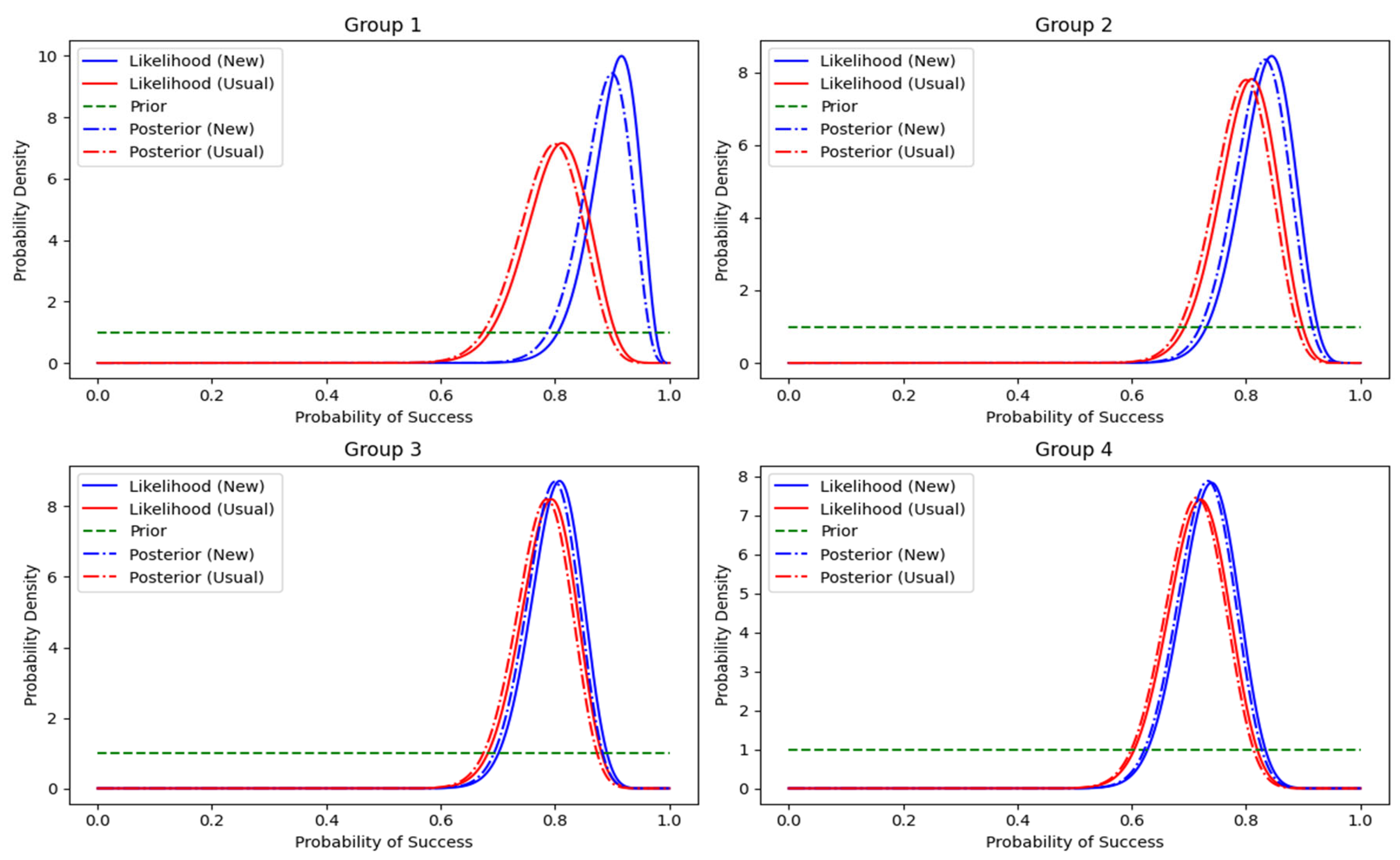
- Figure 4 shows the likelihood, prior, and posterior probabilities for each group so that the two methods may be compared.
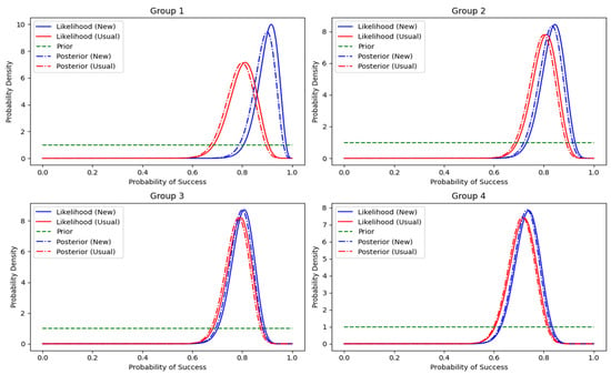 Figure 4. Bayesian inference—likelihood, prior and posterior probability—comparison between usual and new approach.
6. Result and Conclusions
In this study, the kind of conic section and its center are determined through the use of partial differential equations. An introduction differential equation is used in finding the slope as a basic result. The methodology is briefed with few examples. By extension, partial differential equation is used in determining the center of the conic section. The methodology is explained with few examples. To analyze the ease of the methodology, the working procedure was taught to different set of learners. As a result, 90% of the learners were able to learn the new working procedure. In the second attempt, they were able to complete 100% of it. Additionally, they found this methodology comparatively easier than the traditional one. Consequently, they were able to find the slope of any curve easily. To solve the above problem using the normal method, we would have to solve it in the form of a normal ellipse/hyperbola equation. This cannot be achieved easily, and we need to solve it using a trial-and-error method, which can also be used to find the equations of directrix easily. The advantage of using Bayesian inference for this purpose is that it allows incorporating prior beliefs into the analysis. This can be important, as prior beliefs can reflect knowledge of the subject matter, our experience as educators, and our intuition about how students learn. Another advantage of Bayesian inference is that it allows us to make inferences about the relative effectiveness of the two methods, even if there is only a small amount of data. This is because Bayesian methods use all the available data, including prior beliefs, to make inferences.
Author Contributions
Conceptualization, R.D., and S.V.; methodology, C.K.K.; validation, C.P.M.S.S.; formal analysis investigation, K.V.; writing—original draft preparation, R.S. and S.V.; writing—review and editing, R.D. and K.V. All authors have read and agreed to the published version of the manuscript.
Funding
This research received no external funding.
Institutional Review Board Statement
Not applicable.
Informed Consent Statement
Not applicable.
Data Availability Statement
Data can be obtained from the first author on request.
Conflicts of Interest
The authors declare no conflicts of interest.
References
- Friedman, A.; Reitich, F. Analysis of a mathematical model for the growth of tumors. J. Math. Biol. 1999, 38, 262–284. [Google Scholar] [CrossRef]
- Berthier, N.E. Learning to reach: A mathematical model. Dev. Psychol. 1996, 32, 811. [Google Scholar] [CrossRef]
- Crouch, R.; Haines, C. Mathematical modelling: Transitions between the real world and the mathematical model. Int. J. Math. Educ. Sci. Technol. 2004, 35, 197–206. [Google Scholar] [CrossRef]
- Azzoni, A.; La Barbera, G.; Zaninetti, A. Analysis and prediction of rock falls using a mathematical model. Int. J. Rock Mech. Min. Sci. Geomech. Abstr. 1995, 32, 709–724. [Google Scholar] [CrossRef]
- Pfaffl, M.W. A new mathematical model for relative quantification in real-time RT–PCR. Nucleic Acids Res. 2001, 29, 45. [Google Scholar] [CrossRef] [PubMed]
- Nielsen, J.; Landauer, T.K. A mathematical model of the finding of usability problems. In Proceedings of the INTERACT’93 and CHI’93 Conference on Human Factors in Computing Systems, Amsterdam, The Netherlands, 24–29 April 1993; pp. 206–213. [Google Scholar]
- Brantingham, P.J.; Kuhn, S.L. Constraints on Levallois core technology: A mathematical model. J. Archaeol. Sci. 2001, 28, 747–761. [Google Scholar] [CrossRef]
- Brach, R.M.; Dunn, P.F. A mathematical model of the impact and adhesion of microsphers. Aerosol Sci. Technol. 1992, 16, 51–64. [Google Scholar] [CrossRef]
- Kuo, C.C.J. Understanding convolutional neural networks with a mathematical model. J. Vis. Commun. Image Represent. 2016, 41, 406–413. [Google Scholar] [CrossRef]
- Dutta, D.; Herath, S.; Musiake, K. A mathematical model for flood loss estimation. J. Hydrol. 2003, 277, 24–49. [Google Scholar] [CrossRef]
- Martin, J.C.; Milliken, D.L.; Cobb, J.E.; McFadden, K.L.; Coggan, A.R. Validation of a mathematical model for road cycling power. J. Appl. Biomech. 1998, 14, 276–291. [Google Scholar] [CrossRef]
- Roose, T.; Fowler, A.C.; Darrah, P.R. A mathematical model of plant nutrient uptake. J. Math. Biol. 2001, 42, 347–360. [Google Scholar] [CrossRef] [PubMed]
- Heragu, S.S.; Du, L.; Mantel, R.J.; Schuur, P.C. Mathematical model for warehouse design and product allocation. Int. J. Prod. Res. 2005, 43, 327–338. [Google Scholar] [CrossRef]
- LeGrice, I.J.; Hunter, P.J.; Smaill, B.H. Laminar structure of the heart: A mathematical model. Am. J. Physiol.-Heart Circ. Physiol. 1997, 272, 2466–2476. [Google Scholar] [CrossRef] [PubMed]
- Panetta, J.C.; Adam, J. A mathematical model of cycle-specific chemotherapy. Math. Comput. Model. 1995, 22, 67–82. [Google Scholar] [CrossRef]
- Huang, L. Optimization of a new mathematical model for bacterial growth. Food Control 2013, 32, 283–288. [Google Scholar] [CrossRef]
- Xiong, R.; Xie, G.; Edmondson, A.E.; Sheard, M.A. A mathematical model for bacterial inactivation. Int. J. Food Microbiol. 1999, 46, 45–55. [Google Scholar] [CrossRef]
- Chitnis, N.; Hyman, J.M.; Cushing, J.M. Determining important parameters in the spread of malaria through the sensitivity analysis of a mathematical model. Bull. Math. Biol. 2008, 70, 1272. [Google Scholar] [CrossRef]
- Fussenegger, M.; Bailey, J.E.; Varner, J. A mathematical model of caspase function in apoptosis. Nat. Biotechnol. 2000, 18, 768–774. [Google Scholar] [CrossRef]
- Culshaw, R.V.; Ruan, S. A delay-differential equation model of HIV infection of CD4+ T-cells. Math. Biosci. 2000, 165, 27–39. [Google Scholar] [CrossRef]
- Villasana, M.; Radunskaya, A. A delay differential equation model for tumor growth. J. Math. Biol. 2003, 47, 270–294. [Google Scholar] [CrossRef]
- Spencer, S.L.; Berryman, M.J.; Garcia, J.A.; Abbott, D. An ordinary differential equation model for the multistep transformation to cancer. J. Theor. Biol. 2004, 231, 515–524. [Google Scholar] [CrossRef] [PubMed]
- Garcia, O. A stochastic differential equation model for the height growth of forest stands. Biometrics 1983, 39, 1059–1072. [Google Scholar] [CrossRef]
- Smith, D.; Moore, L. The SIR model for spread of disease—The differential equation model. Convergence Math. Assoc. Am. 2004, 1–4. [Google Scholar]
- Chen, K.C.; Wang, T.Y.; Tseng, H.H.; Huang, C.Y.F.; Kao, C.Y. A stochastic differential equation model for quantifying transcriptional regulatory network in Saccharomyces cerevisiae. Bioinformatics 2005, 21, 2883–2890. [Google Scholar] [CrossRef] [PubMed]
- Gourley, S.A.; Kuang, Y.; Nagy, J.D. Dynamics of a delay differential equation model of hepatitis B virus infection. J. Biol. Dyn. 2008, 2, 140–153. [Google Scholar] [CrossRef] [PubMed]
- Deboeck, P.R.; Bergeman, C.S. The reservoir model: A differential equation model of psychological regulation. Psychol. Methods 2013, 18, 237. [Google Scholar] [CrossRef] [PubMed]
- Chattopadhyay, J.; Sarkar, R.R.; El Abdllaoui, A. A delay differential equation model on harmful algal blooms in the presence of toxic substances. Math. Med. Biol. J. IMA 2002, 19, 137–161. [Google Scholar] [CrossRef]
- Unami, K.; Abagale, F.K.; Yangyuoru, M.; Alam, A.H.M.B.; Kranjac-Berisavljevic, G. A stochastic differential equation model for assessing drought and flood risks. Stoch. Environ. Res. Risk Assess. 2010, 24, 725–733. [Google Scholar] [CrossRef]
- Tamura, Y.; Yamada, S. A flexible stochastic differential equation model in distributed development environment. Eur. J. Oper. Res. 2006, 168, 143–152. [Google Scholar] [CrossRef]
- Myerscough, M.R.; Gray, B.F.; Hogarth, W.L.; Norbury, J. An analysis of an ordinary differential equation model for a two-species predator-prey system with harvesting and stocking. J. Math. Biol. 1992, 30, 389–411. [Google Scholar] [CrossRef]
- Gennemark, P.; Wedelin, D. Efficient algorithms for ordinary differential equation model identification of biological systems. IET Syst. Biol. 2007, 1, 120–129. [Google Scholar] [CrossRef] [PubMed]
- Salahshour, S.; Ahmadian, A.; Senu, N.; Baleanu, D.; Agarwal, P. On analytical solutions of the fractional differential equation with uncertainty: Application to the Basset problem. Entropy 2015, 17, 885–902. [Google Scholar] [CrossRef]
- Shah, K.; Khalil, H.; Khan, R.A. Investigation of positive solution to a coupled system of impulsive boundary value problems for nonlinear fractional order differential equations. Chaos Solitons Fractals 2015, 77, 240–246. [Google Scholar] [CrossRef]
- Semenova, I.N. Methodology of Teaching Mathematics Methods Designing in the Modern Educational Paradigm; Science Book Publishing House LLC: Yelm, WA, USA, 2014; pp. 1–156. [Google Scholar]
- Izquierdo, N.V.; Viloria, A.; Gaitan-Angulo, M.; Bonerg, O.; Lezama, P.; Erase, J.J.C.; Gutierrez, A.S. Methodology of application of diffuse mathematics to performance evaluation. Int. J. Control Theory Appl. 2016, 9, 201–207. [Google Scholar]
- Nortvedt, G.A.; Buchholtz, N. Assessment in mathematics education: Responding to issues regarding methodology, policy, and equity. ZDM—Math. Educ. 2018, 50, 555–570. [Google Scholar] [CrossRef]
- Asiedu-Addo, S.K.; Yidana, I. Mathematics teachers’ knowledge of the subject content and methodology. Math. Connect. 2004, 4, 45–51. [Google Scholar] [CrossRef]
Disclaimer/Publisher’s Note: The statements, opinions and data contained in all publications are solely those of the individual author(s) and contributor(s) and not of MDPI and/or the editor(s). MDPI and/or the editor(s) disclaim responsibility for any injury to people or property resulting from any ideas, methods, instructions or products referred to in the content. |
© 2023 by the authors. Licensee MDPI, Basel, Switzerland. This article is an open access article distributed under the terms and conditions of the Creative Commons Attribution (CC BY) license (https://creativecommons.org/licenses/by/4.0/).

