
An Innovative Ranking Method for Hexagonal Intuitionistic Fuzzy Transportation Issues †

Abstract
1. Introduction
2. Preliminaries
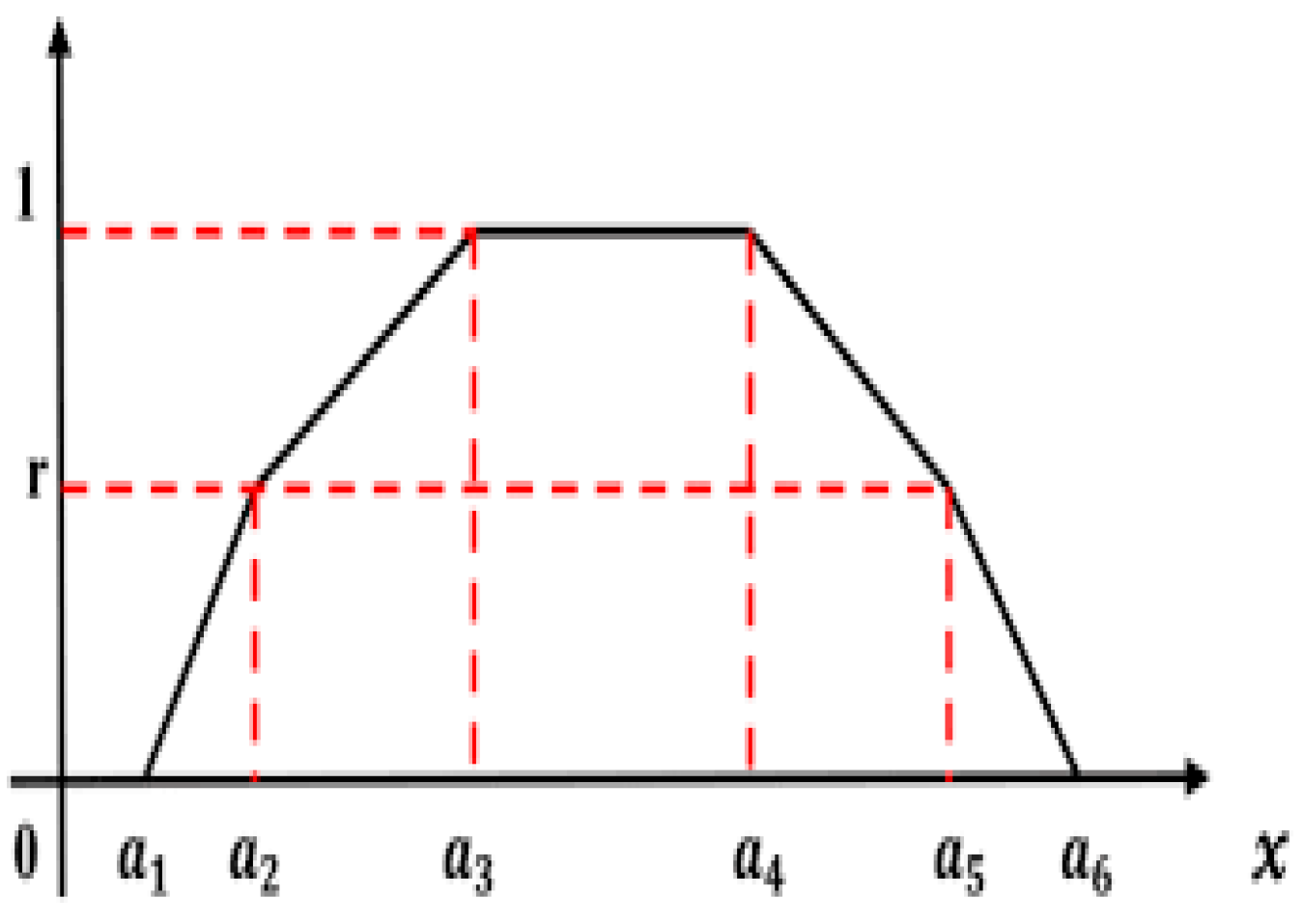
- has a continuous piece-wise pattern.
- appears to be a convex fuzzy subgroup.
- represents a fuzzy subset of a piecewise continuous pattern, indicating that the value originally filled for a minimum of one member must be 1, that is, .
3. The Proposed Ranking Approach for HIFNs
4. Comparison of HIFNs
- (i)
- (ii)
- (iii)
- (i)
- (ii)
- .
Mathematical Formulation of Hexagonal Intuitionistic Fuzzy Transportation Problem (HIFTP)
5. Transportation Strategy
5.1. Proposed Transportation Strategy
6. Numerical Example
7. Conclusions
Author Contributions
Funding
Institutional Review Board Statement
Informed Consent Statement
Data Availability Statement
Conflicts of Interest
References
- Atanassov, K.T. Intuitionistic fuzzy sets. Fuzzy Sets Syst. 1986, 20, 87–96. [Google Scholar] [CrossRef]
- Atanassov, K.T. Intuitionistic Fuzzy Sets: Theory and Applications; Physica Verlag: Heidelberg, Germany; New York, NY, USA, 1999. [Google Scholar]
- Bellmann, R.E.; Zadeh, L.A. Decision making in fuzzy environment. Manag. Sci. 1970, 17, 141–164. [Google Scholar] [CrossRef]
- Rout, A.; Bbvl, D.; Biswal, B.B.; Mahanta, G.B. A fuzzy-regression-PSO based hybrid method for selecting welding conditions in robotic gas metal arc welding. Assem. Autom. 2020, 40, 601–612. [Google Scholar] [CrossRef]
- Hussain, R.J.; Senthil Kumar, P. Algorithm approach for solving intuitionistic fuzzy transportation problem. Appl. Math. Sci. 2012, 6, 3981–3989. [Google Scholar]
- Nagoor Gani, A.; Abbas, S. A New method for solving Intuitionistic Fuzzy Transportation problem using zero suffix algorithm. Int. J. Math. Sci. Eng. 2012, 6, 73–82. [Google Scholar]
- Nagoor Gani, A.; Abbas, S. A New method for solving Intuitionistic Fuzzy Transportation problem. Appl. Math. Sci. 2013, 7, 1357–1365. [Google Scholar]
- O’heigeartaigh, H. A fuzzy transportation algorithm. Fuzzy Sets Syst. 1982, 8, 235–243. [Google Scholar] [CrossRef]
- Pandian, P.; Natarajan, G. A new algorithm for finding a fuzzy optimal solution for fuzzy transportation problem. Appl. Math. Sci. 2010, 4, 79–90. [Google Scholar]
- Rout, A.; Mahanta, G.B.; Biswal, B.B.; Vardhan Raj, S.; BBVL, D. Application of fuzzy logic in multi-sensor-based health service robot for condition monitoring during pandemic situations. Robot. Intell. Autom. 2024, 44, 96–107. [Google Scholar] [CrossRef]
- Rajarajeswari, P.; Sahaya Sudha, A. Ranking of Hexagonal Fuzzy Numbers using Centroid. AARJMD 2014, 1, 265–277. [Google Scholar]
- Zadeh, L.A. Fuzzy sets. Inf. Control 1965, 8, 338–353. [Google Scholar] [CrossRef]


| 5 | 6 | 12 | 9 | (7,9,11,13,16,20) (5,7,11,13,19,23) | |
| 3 | 2 | 8 | 4 | (6,8,11,14,19,25) (4,7,11,14,21,27) | |
| 7 | 11 | 20 | 9 | (9,11,13,15,18,20) (8,10,13,15,19,22) | |
| (3,4,5,6,8,10) (2,4,5,6,10,12) | (3,5,7,9,12,15) (2,4,7,9,13,17) | (6,7,9,11,13,16) (5,6,9,11,16,18) | (10,12,14,16,20,24) (8,10,14,16,20,25) |
| Row Diff. | ||||||
|---|---|---|---|---|---|---|
| 5 | 6 | 12 | 9 | (7,9,11,13,16,20) (5,7,11,13,19,23) | 1 | |
| 3 | 2 | 8 | 4 | (6,8,11,14,19,25) (4,7,11,14,21,27) | 1 | |
| 7 | 11 | 20 | 9 | (9,11,13,15,18,20) (8,10,13,15,19,22) | 4 | |
| (3,4,5,6,8,10) (2,4,5,6,10,12) | (3,5,7,9,12,15) (2,4,7,9,13,17) | (6,7,9,11,13,16) (5,6,9,11,16,18) | (10,12,14,16,20,24) (8,10,14,16,20,25) | 6 | ||
| Col. Diff | 2 | 4 | 4 | 5 | C = 15 | R = 12 |
| 5 | 6 | 12 | 9 | (7,9,11,13,16,20) (5,7,11,13,19,23) | |
| 3 | 2 | 8 | 4 (6,8,11,14,19,25) (4,7,11,14,21,27) | 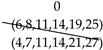 | |
| 7 | 11 | 20 | 9 | (9,11,13,15,18,20) (8,10,13,15,19,22) | |
| (3,4,5,6,8,10) (2,4,5,6,10,12) | (3,5,7,9,12,15) (2,4,7,9,13,17) | (6,7,9,11,13,16) (5,6,9,11,16,18) | (−15,−7,0,5,12,18) (−19,−11,0,5,13,21) |
| 5 | 6 | 12 | 9 | (7,9,11,13,16,20) (5,7,11,13,19,23) | |
| 7 | 11 | 20 | 9 | (9,11,13,15,18,20) (8,10,13,15,19,22) | |
| (3,4,5,6,8,10) (2,4,5,6,10,12) | (3,5,7,9,12,15) (2,4,7,9,13,17) | (6,7,9,11,13,16) (5,6,9,11,16,18) | (−15,−7,0,5,12,18) (−19,−11,0,5,13,21) |
| Row Diff | ||||||
|---|---|---|---|---|---|---|
| 5 | 6 | 12 | 9 | (7,9,11,13,16,20) (5,7,11,13,19,23) | 1 | |
| 7 | 11 | 20 | 9 | (9,11,13,15,18,20) (8,10,13,15,19,22) | 2 | |
| (3,4,5,6,8,10) (2,4,5,6,10,12) | (3,5,7,9,12,15) (2,4,7,9,13,17) | (6,7,9,11,13,16) (5,6,9,11,16,18) | (−15,−7,0,5,12,18) (−19,−11,0,5,13,21) | C = 3 | ||
| Col. Diff | 2 | 5 | 8 | 0 | R = 15 |
| 5 | 6 (−9,−4,0,4,9,14) (−13,−9,0,4,13,18) | 12 (6,7,9,11,13,16) (5,6,9,11,16,18) | 9 | |
| 3 | 2 | 8 | 4 (6,8,11,14,19,25) (4,7,11,14,21,27) | |
| 7 (3,4,5,6,8,10) (2,4,5,6,10,12) | 11 (−11,−4,3,9,16,24) (−16,−9,3,9,22,30) | 20 (−15,−7,0,5,12,18) (−19,−11,0,5,13,21) | 9 |
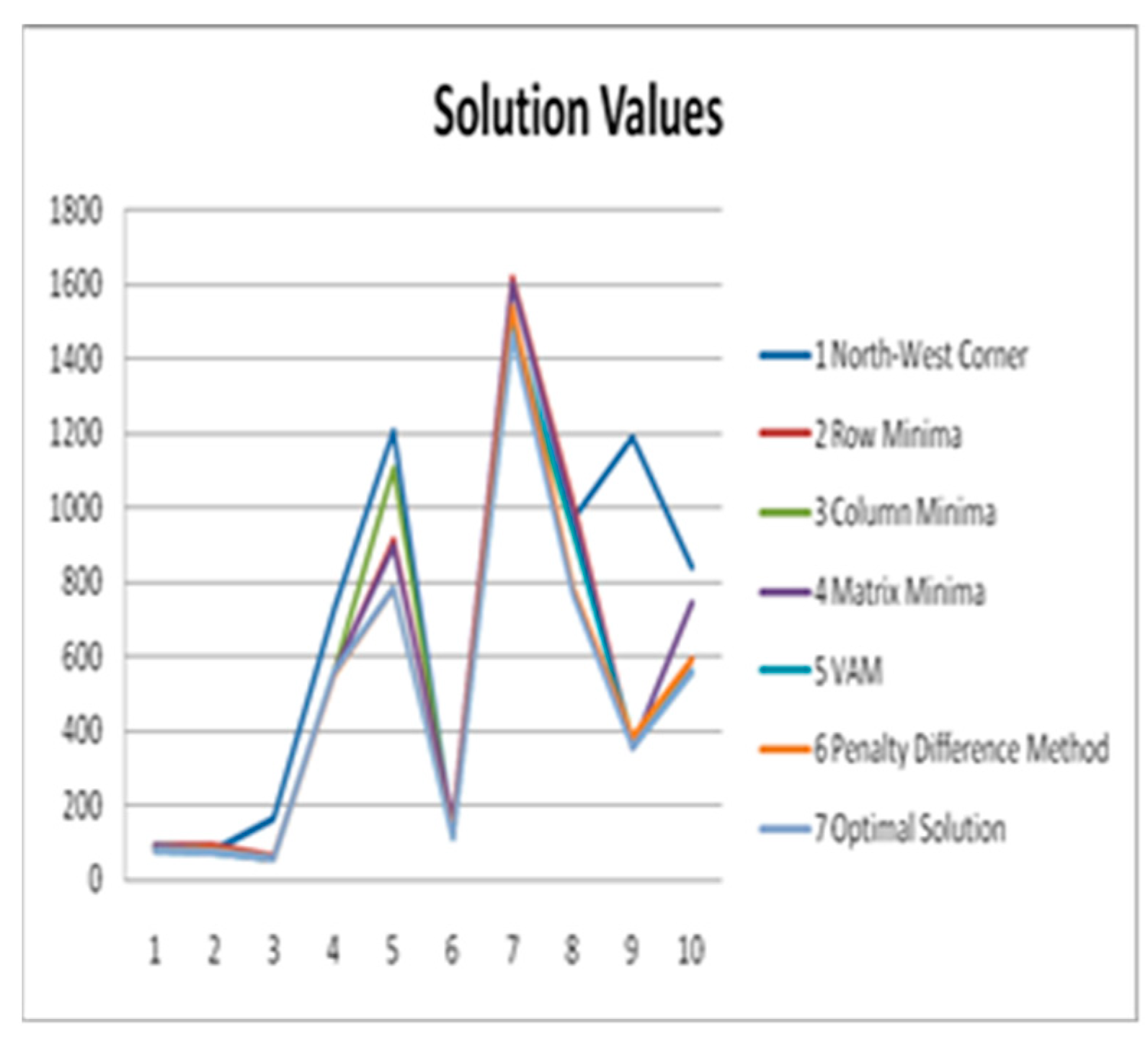
| Name of the Method | North–West Corner | Row Minima | Column Minima | Matrix Minima | VAM | Penalty Difference Algorithm | Optimum Cost |
|---|---|---|---|---|---|---|---|
| Problem 1 | 90 | 92 | 92 | 92 | 76 | 76 | 76 |
| Deviation % | 0.18 | 0.21 | 0.21 | 0.21 | 0.00 | 0.00 | 0.00 |
| Problem 2 | 82 | 88 | 77 | 77 | 73 | 77 | 73 |
| Deviation % | 0.12 | 0.21 | 0.05 | 0.05 | 0.00 | 0.05 | 0.00 |
| Problem 3 | 167 | 61 | 56 | 56 | 56 | 56 | 56 |
| Deviation % | 1.98 | 0.09 | 0.00 | 0.00 | 0.00 | 0.00 | 0.00 |
| Problem 4 | 730 | 555 | 555 | 555 | 555 | 555 | 555 |
| Deviation % | 0.32 | 0.00 | 0.00 | 0.00 | 0.00 | 0.00 | 0.00 |
| Problem 5 | 1207 | 916 | 1102 | 896 | 782 | 782 | 782 |
| Deviation % | 0.54 | 0.17 | 0.41 | 0.15 | 0.00 | 0.00 | 0.00 |
| Problem 6 | 128 | 152 | 121 | 156 | 114 | 123 | 114 |
| Deviation % | 0.12 | 0.33 | 0.06 | 0.37 | 0.00 | 0.08 | 0.00 |
| Problem 7 | 1615 | 1620 | 1465 | 1600 | 1510 | 1540 | 1465 |
| Deviation % | 0.10 | 0.11 | 0.00 | 0.09 | 0.03 | 0.05 | 0.00 |
| Problem 8 | 974 | 1014 | 931 | 984 | 936 | 783 | 768 |
| Deviation % | 0.27 | 0.32 | 0.21 | 0.28 | 0.22 | 0.02 | 0.00 |
| Problem 9 | 1195 | 355 | 380 | 355 | 355 | 385 | 355 |
| Deviation % | 2.37 | 0.00 | 0.07 | 0.00 | 0.00 | 0.08 | 0.00 |
| Problem 10 | 845 | 590 | 555 | 745 | 555 | 590 | 555 |
| Deviation % | 0.52 | 0.06 | 0.00 | 0.34 | 0.00 | 0.06 | 0.00 |
| Number of best solution | 0 | 2 | 3 | 3 | 8 | 5 | |
| Mean deviation (%) | 0.65 | 0.15 | 0.10 | 0.15 | 0.03 | 0.03 |
Disclaimer/Publisher’s Note: The statements, opinions and data contained in all publications are solely those of the individual author(s) and contributor(s) and not of MDPI and/or the editor(s). MDPI and/or the editor(s) disclaim responsibility for any injury to people or property resulting from any ideas, methods, instructions or products referred to in the content. |
© 2024 by the authors. Licensee MDPI, Basel, Switzerland. This article is an open access article distributed under the terms and conditions of the Creative Commons Attribution (CC BY) license (https://creativecommons.org/licenses/by/4.0/).
Share and Cite
Singuluri, I.; Nemani, R.; Swetha, C.U. An Innovative Ranking Method for Hexagonal Intuitionistic Fuzzy Transportation Issues. Eng. Proc. 2024, 66, 44. https://doi.org/10.3390/engproc2024066044
Singuluri I, Nemani R, Swetha CU. An Innovative Ranking Method for Hexagonal Intuitionistic Fuzzy Transportation Issues. Engineering Proceedings. 2024; 66(1):44. https://doi.org/10.3390/engproc2024066044
Chicago/Turabian StyleSinguluri, Indira, Ramya Nemani, and CH. Uma Swetha. 2024. "An Innovative Ranking Method for Hexagonal Intuitionistic Fuzzy Transportation Issues" Engineering Proceedings 66, no. 1: 44. https://doi.org/10.3390/engproc2024066044
APA StyleSinguluri, I., Nemani, R., & Swetha, C. U. (2024). An Innovative Ranking Method for Hexagonal Intuitionistic Fuzzy Transportation Issues. Engineering Proceedings, 66(1), 44. https://doi.org/10.3390/engproc2024066044