Impact of Climate Change on the Thermoeconomic Performance of Binary-Cycle Geothermal Power Plants ^†

Abstract

The thermoeconomic performance of geothermal power plants is influenced by a variety of site-specific factors, major economic variables, and the type of the involved technology. In addition to those, ambient conditions also play a role in geothermal power generation by acting on the cooling towers. This study focuses on the performance analysis of a binary cycle with isobutane for geothermal power generation under the impact of climate change. Long-term temperature variations in ambient air are described by temperature anomalies under two shared socioeconomic pathways (SSP). These are the intermediate SSP2-4.5 scenario and the extreme SSP5-8.5 scenario, over the period from 2021 to 2100. Different climate models from the most recent Climate Model Intercomparison Project (CMIP6) are compared against each other and against the observed temperature data. The predictive power of the CMIP6 climate models is evaluated using the root mean square error (RMSE) and the Kullback–Leibler (KL) criteria. The thermoeconomic performance of the geothermal power plant is expressed in terms of net power output, annual electricity generation (AEG), and levelized cost of electricity (LCOE). The geothermal power plant achieves a net power output of 10 MW and an LCOE of 79.2 USD/MWh for an ambient air temperature of 12 °C. This temperature is the average temperature over the reference period of 1991–2020 in Bjelovar, Croatia (45.8988° N, 16.8423° E). Under the impact of climate change, the same geothermal power plant will have the AEG reduced by between 0.5% and 2.9% in the intermediate (SSP2-4.5) scenario and by between 2.0% and 8.7% in the extreme (SSP5-8.5) scenario. The LCOE will increase between 0.4% and 1.8% in the intermediate scenario and from 1.3% to 5.6% in the extreme scenario.

1. Introduction

A general misconception is that geothermal energy is an infinite resource of renewable energy and that geothermal power plants operate with zero environmental impact. However, the overdevelopment of geothermal resources can cause accelerated depletion and productivity decline. For instance, electricity generation from the Geysers geothermal field in California started to decline after excessive extraction of dry steam in the 1980s. In 1987, the Geysers power plants operated with an average net capacity between 1500 and 1600 MW, and the capacity factor was between 91 and 97% relative to the net nameplate capacity of 1640 MW. After that, net generation dropped by more than 40%, and net generation capacity was less than 900 MW by 1995. Augmented injection of steam condensate and surface runoff was implemented, aiming to boost the rechange rates of the Geysers field and stabilize electricity generation [1]. In 2022, the Geysers power plants generated 5847 GWh of electricity, equal to an average net capacity of 835 MW, assuming 7000 full load hours per year [2]. Concerning greenhouse gas emissions (expressed in kg of CO₂ equivalents), geothermal power plants operate at an average global emission rate of 122 kg/MWh. The emissions from geothermal sources exhibit high variability and depend on the reservoir properties, as well as on the technologies involved in extracting the energy content from the geothermal fluid. The New Zealand Geothermal Association reports that geothermal power plants in New Zealand emit between 21 and 341 kg_CO2/MWh, with a weighted average of 76 kg_CO2-eq/MWh [3]. Recent data from other countries shows that the emissions from geothermal power plants were 34 kg/kWh in Iceland, 107 kg/kWh in California, and 330 kg/kWh in Italy [4].

Climate change and extreme weather events will affect the reliability and availability of electricity generation from renewable energy sources, both on the supply side and on the demand side [5]. On the supply side, changing rainfall quantities and wind patterns will impact hydropower [6,7] and wind-power [8,9] generation. Increasing air temperatures and prolonged droughts will affect the efficiency of cooling systems in nuclear, thermal, and geothermal power plants, even forcing shutdowns in periods of extreme heat [10]. Extreme weather events, such as wildfires, floods, hurricanes, and storms will damage the electricity transmission and distribution infrastructure, leading to power outages [11,12]. On the demand side, hotter summers will increase cooling and air-conditioning energy demand [13], while milder winters may reduce the need for heating [14].

The general assertion is that climate change will not affect geothermal energy because geothermal energy is influenced by the structure and physical processes within the Earth’s interior [15]. Ground-source heat pumps should remain unaffected by climate change because their performance will adapt to the gradual changes in ambient temperatures through technological development [16]. However, climate change could affect heat rejection systems in nuclear, thermal, and geothermal power plants, causing a decline in electricity generation. Linnerud et al. [17] estimated that the loss of electricity generation could be more than 2.0% for each degree Celsius of global warming in nuclear power plants. Petrakopoulou et al. [18] determined that a 10 °C increase in ambient temperature would increase the steam turbine outlet pressure by 43–60% and reduce coal power-plant efficiency in the range between 0.3 and 0.7% pts., depending on the cooling-system type. Canales et al. [19] conclude that climate change will impact shallow geothermal resources and ground-source heat pumps. Warmer future climates may also impact the performance of air-cooled chillers supplying cooling energy for buildings [20].

Furthermore, climate change could affect the availability and productivity of geothermal resources. Changes in precipitation patterns and prolonged droughts may affect groundwater levels. This, in turn, could slow down the recharge rates of wells and reduce geothermal electricity generation. For example, geothermal power generation in the tropical regions of the Pacific Ocean may be at risk of more frequent and intensive El Niño–Southern Oscillation (ENSO) events [21]. The El Niño phenomenon is expected to cause longer periods of drought, resulting in severe water shortages and competing water use between geothermal projects and agricultural communities. Geothermal drilling operations and the power-plant availability factors may be seriously affected as a result. Generally, the El Niño is followed by the La Niña event, which is marked by intense rainfalls over short periods of time. This could affect geothermal energy through increased risk of floods in plains and valleys and landslides in mountain regions.

The aim of this work is to quantify the impact of climate change on the thermal and economic performance of a binary-cycle power plant using an air-cooled condenser. The analysis is performed for two representative climate-change scenarios, namely the intermediate scenario (SSP2-4.5) and the extreme scenario (SSP5-8.5), over the period from 2021 to 2100.

2. Methods

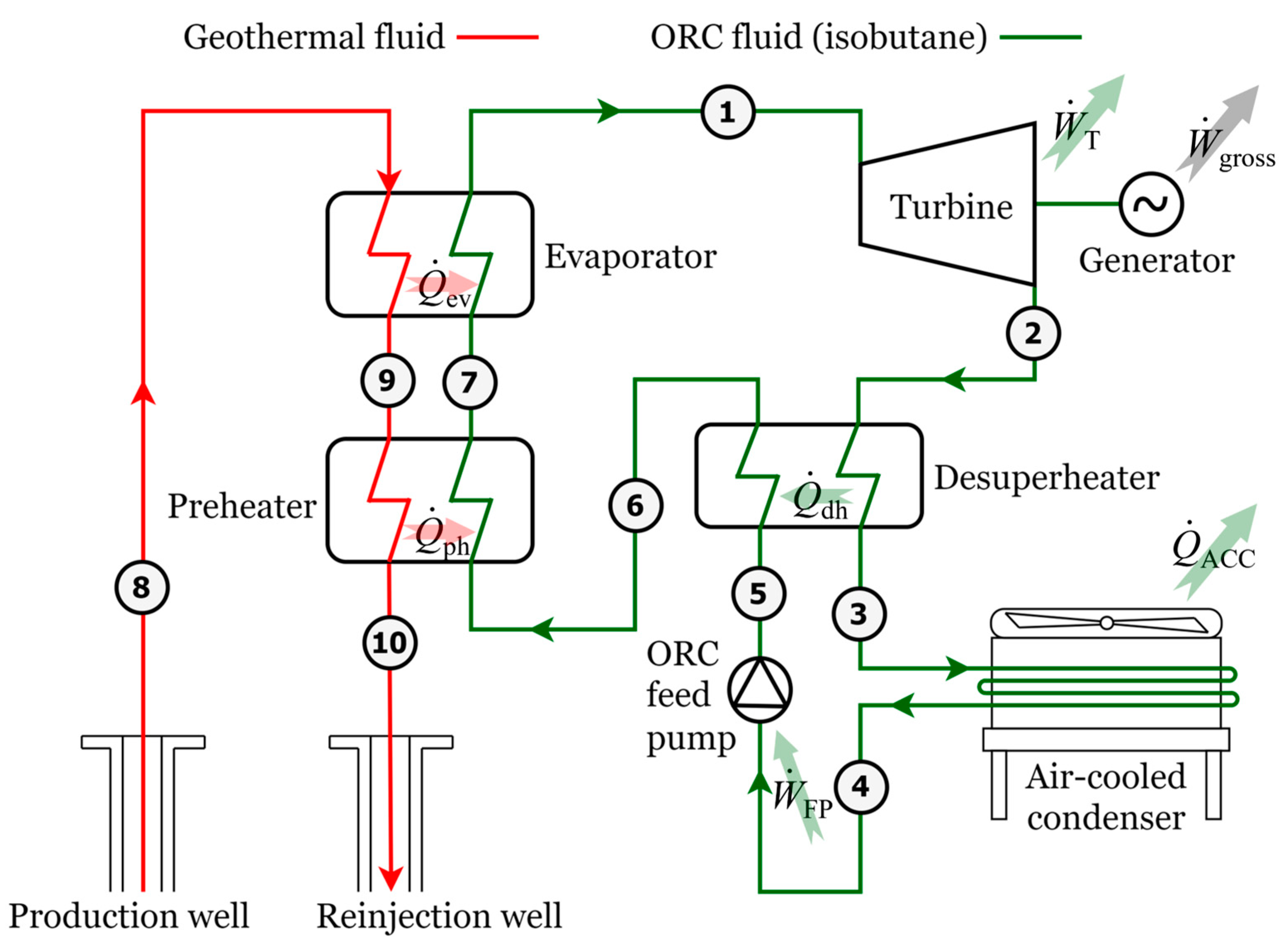
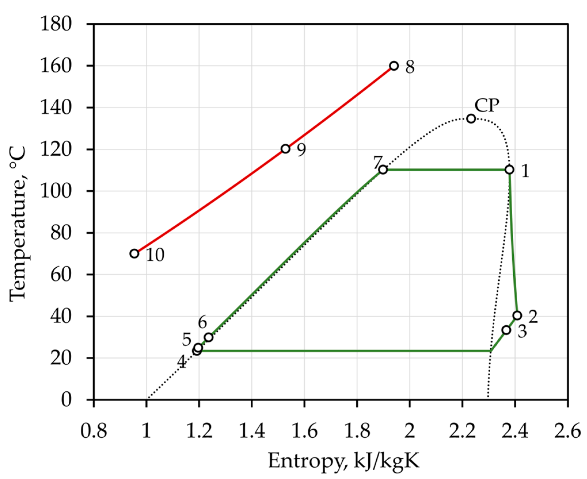
2.1. Thermodynamic Model

The geothermal power plant is modeled as an Organic Rankine Cycle (ORC) single-stage configuration using isobutane as the working fluid. The geothermal fluid flows from the production well, with a temperature of 160 °C, a pressure of 25 bar, and a mass flow rate of 225 kg/s (state ⑧). Thermal energy is transferred to isobutane in the preheater, ⑨ → ⑩, and evaporator, ⑧ → ⑨, as shown in Figure 1. Isobutane flows in a closed loop and runs the ORC turbine, ① → ②. Isobutane condenses inside the air-cooled condenser, ③ → ④. The ORC feed pump ensures the pressure difference in the isobutane circuit, ④ → ⑤. The desuperheater recovers the sensible heat content, ⑤ → ⑥, from the exhaust vapor of the turbine, ② → ③. This is because, unlike water vapor, isobutane is a dry working fluid, and its expansion ends in the superheated region.

The thermodynamic model applies mass and energy conservation equations to the major components of the binary cycle (heat exchangers, pumps, and turbines). The heating duty of the evaporator and preheater are

$${\dot{Q}}_{\mathrm{ev}}={\dot{m}}_{\mathrm{ORC}}\left(h_1-h_7\right)={\dot{m}}_{\mathrm{GTF}}\left(h_8-h_9\right){\eta }_{\mathrm{EV}}$$

(1)

$${\dot{Q}}_{\mathrm{ph}}={\dot{m}}_{\mathrm{ORC}}\left(h_7-h_6\right)={\dot{m}}_{\mathrm{GTF}}\left(h_9-h_{10}\right){\eta }_{\mathrm{PH}}$$

(2)

The heating duty of the desuperheater and air-cooled condenser are:

$${\dot{Q}}_{\mathrm{dh}}={\dot{m}}_{\mathrm{ORC}}\left(h_2-h_3\right){\eta }_{\mathrm{RE}}={\dot{m}}_{\mathrm{ORC}}\left(h_6-h_5\right)$$

(3)

$${\dot{Q}}_{\mathrm{ACC}}={\dot{m}}_{\mathrm{ORC}}\left(h_3-h_4\right)={\dot{m}}_{\mathrm{air}}\left(h_{\mathrm{a},\mathrm{out}}-h_{\mathrm{a},\mathrm{in}}\right)$$

(4)

Heat losses from the evaporator and the preheater to the ambient are assumed as 10% of the total heating duty (η_EV = 0.90, η_PH = 0.90), reflecting the non-ideal thermal insulation of the heat exchangers and piping [22]. Heat losses in the desuperheater are 5% (η_RE = 0.95). To prevent silica precipitation, a minimum reinjection temperature of 70 °C was assumed. The minimum pinch-point temperature difference between the geothermal fluid and the ORC fluid is 10 °C. The turbine and the feed pump power duties are calculated as

$${\dot{W}}_{\mathrm{T}}={\dot{m}}_{\mathrm{ORC}}\left(h_1-h_2\right)={\dot{m}}_{\mathrm{ORC}}\left(h_1-h_{2,\mathrm{is}}\right){\eta }_{\mathrm{T}}$$

(5)

$${\dot{W}}_{\mathrm{FP}}={\dot{m}}_{\mathrm{ORC}}\left(h_5-h_4\right)={\displaystyle \frac{{\dot{m}}_{\mathrm{ORC}}\left(h_{5,\mathrm{is}}-h_4\right)}{{\eta }_{\mathrm{FP}}}}$$

(6)

The isentropic efficiencies of the turbine and feed pump are assumed to be constant and equal to η_T = 0.88 and η_FP = 0.75, respectively. The high efficiencies of the turbine and feed pump are achieved with a dedicated design [23], while their constant values assume design point operation all the time. The gross electricity output of the power plant is obtained by reducing the turbine power duty for electrical and mechanical losses by 2% each. That is, η_m = 0.98 and η_el = 0.98

$${\dot{W}}_{\mathrm{gross}}={\dot{W}}_{\mathrm{T}}{\eta }_{\mathrm{m}}{\eta }_{\mathrm{el}}$$

(7)

Net electricity output is obtained by subtracting the feed pump and auxiliary duties (cooling tower fans and reinjection pump) from the gross electricity output. That is,

$${\dot{W}}_{\mathrm{net}}={\dot{W}}_{\mathrm{gross}}-\left({\dot{W}}_{\mathrm{FP}}+{\dot{W}}_{\mathrm{AUX}}\right)$$

(8)

In (8), auxiliary power is assumed equal to 5% of the gross electricity output (W_AUX = 0.05 × W_gross). The annual net electricity generation is calculated assuming N_FLH = 7000 full load hours per year, equivalent to an average capacity factor of 80%.

$$E_{\mathrm{net}}={\dot{W}}_{\mathrm{net}}·N_{\mathrm{FLH}}$$

(9)

The net efficiency of the geothermal power plant is the ratio between the net electricity output and the maximum available heating duty of the evaporator and preheater.

$${\eta }_{\mathrm{th},\mathrm{net}}={\displaystyle \frac{{\dot{W}}_{\mathrm{net}}}{{\dot{Q}}_{\mathrm{PR}}+{\dot{Q}}_{\mathrm{EV}}}}={\displaystyle \frac{{\dot{W}}_{\mathrm{T}}{\eta }_{\mathrm{m}}{\eta }_{\mathrm{el}}-({\dot{W}}_{\mathrm{FP}}+{\dot{W}}_{\mathrm{AUX}})}{{\dot{m}}_{\mathrm{GTF}}·(h_8-h_{10,T=70°\mathrm{C}})}}$$

(10)

The economic performance of the geothermal power plant is estimated with two cost metrics, namely the levelized cost of electricity (LCOE) and the specific installation cost (SIC). The LCOE calculates the net present value of the geothermal power plant, accounting for the capital investment, as well as the costs of operation, maintenance, and materials. Further, the LCOE is corrected by assuming a real cost of capital of r = 5%, a price escalation rate of e = 3%, and a decline rate for annual electricity generation of d = 1%. The power plant’s lifetime is N_y = 25 years.

$$LCOE={\displaystyle \frac{C_{\mathrm{CAP}}+{\displaystyle \sum _{t=1}^{t=N_{\mathrm{y}}}{\left(C_{\mathrm{O}\&\mathrm{M}}+C_{\mathrm{M}}\right)}_t\frac{{\left(1+e\right)}^t}{{\left(1+r\right)}^t}}}{{\displaystyle \sum _{t=1}^{t=N_{\mathrm{y}}}{E}_{\mathrm{net}}{(1-d)}^t}}}$$

(11)

Total capital costs (C_cap) are estimated from initial investment costs (C_init), which include the purchased equipment (turbine, air-cooled condenser, evaporator, preheater, pumps, fans, production, and reinjection well), as well as their installation and other auxiliary costs for a greenfield project (site development, fees and contingencies, auxiliary buildings, and utilities). Initial investment costs are financed using a bank loan at an interest rate of r = 5%. The specific installation costs of the geothermal power plant are calculated as the ratio between the initial investment costs and the net electricity output.

$$SIC={\displaystyle \frac{C_{\mathrm{init}}}{{\dot{W}}_{\mathrm{net}}}}$$

(12)

The ORC configurations shown in Figure 1 achieve a gross and a net power output of 12.1 MW and 10 MW, respectively. The net cycle efficiency is 11.6% at an ambient air temperature is 12 °C. In this case, the levelized cost of electricity (LCOE) is 79.2 USD/MWh, and the SIC is 5400 USD/kW.

The geothermal power plant uses an air-cooled condenser (ACC) to discharge the low-temperature heat into the atmosphere. The flat coil air-cooled condenser is shown in Figure 2. Isobutane enters the condenser as superheated vapor and is distributed through the coil tubes. Fans, which are positioned at the unit top, draw cool ambient air over the coil, augmenting heat transfer. Liquid-state isobutane exits the unit via the outlet header.

Unlike wet cooling towers, which rely on sensible and latent heat exchange (evaporative cooling), dry cooling towers or air-cooled condensers rely solely on sensible heat transfer. Consequently, ACCs are typically less efficient, of bigger size, and occupy more land area than wet cooling towers. However, ACCs do not require a dedicated source of fresh make-up water to replace evaporative losses from the tower. This makes them the preferred option in regions with limited water availability and cold climates. In regions with cold winters, wet cooling towers need to be equipped with electric heaters, additional thermal insulation, and antifreeze additives to prevent freezing problems and power-plant shut-downs. The heat-balance equation between isobutane and air is given with Equation (4), while the heat transfer equation of the ACC is:

$${\dot{Q}}_{\mathrm{ACC}}=U·{\left(N·A\right)}_{\mathrm{unit}}·\Delta T_{\log }$$

(13)

The ACC consists of the N unit cells, each with a 1 MW rated capacity, that are necessary to achieve the total heat rejection rate. The heat-transfer surface area of the unit cell (A_unit) is determined by manufacturer data [24]. The thermal sizing problem requires balancing the temperature difference (ΔT_log) with the heat-transfer coefficient (U) to achieve the 1 MW rated capacity of a unit cell. In ACCs, the dominant thermal resistance is on the air side (R_air), and the U-value depends mostly on the air-side velocity. However, the air velocity must be limited to prevent excessive ventilation load, which would affect the geothermal power plant’s performance. Now, as the U-value is limited by the air-side velocity, the temperature difference between isobutane and air is increased until the unit cell achieves the rated capacity. The log-mean temperature difference is determined from the saturation temperature of isobutane (T_sat) and the air inlet (T_a,in) and outlet (T_a,out) temperatures

$$\Delta T_{\log }={\displaystyle \frac{T_{\mathrm{a},\mathrm{out}}-T_{\mathrm{a},\mathrm{in}}}{\ln \left(\frac{T_{\mathrm{sat}}-T_{\mathrm{a},\mathrm{in}}}{T_{\mathrm{sat}}-T_{\mathrm{a},\mathrm{out}}}\right)}}$$

(14)

The U-value of the ACC is calculated by summing three thermal resistances in series: the air-side convection resistance (R_air), the condensing fluid convection resistance (R_cond), and the conduction resistance for circular tubes with a single-layer wall (R_tube)

$$\underset{R_{\mathrm{total}}}{\underbrace{{\displaystyle \frac{1}{U·A}}}}=\underset{R_{\mathrm{air}}}{\underbrace{{\displaystyle \frac{1}{{(\eta ·h·A)}_{\mathrm{air}}}}}}+\underset{R_{\mathrm{tube}}}{\underbrace{{\displaystyle \frac{\ln (d_{\mathrm{o}}/d_{\mathrm{i}})}{2\pi {(k·L·N)}_{\mathrm{wall}}}}}}+\underset{R_{\mathrm{cond}}}{\underbrace{{\displaystyle \frac{1}{{(h·A)}_{\mathrm{cond}}}}}}$$

(15)

In the above equation, h_air and h_cond are the heat-transfer coefficients on the air and tube side, respectively. The tube material is stainless steel (k = 15 W/m∙K) and that of the fins is aluminum (k = 220 W/m∙K). The tube’s inside diameter is d_i = 14.1 mm and the outside diameter is d_o = 15.9 mm. The transversal and longitudinal tube pitch are equal, that is X_T = X_L = 30 mm. The fin thickness is 0.2 mm, and the fin pitch is 2.3 mm. Each ACC unit subdivides the isobutane flow into 90 flow circuits, with each circuit having 6 tubes (N = 540) in a counterflow arrangement against the incoming airflow.

The ε-NTU approach is used for the thermal sizing of the ACC. The thermal effectiveness (ε) relates to the number of transfer units (NTU) of the evaporator–condenser relationship.

$$\epsilon =1-{\mathrm{e}}^{-NTU},\mathrm{for}C*=C_{\min }/C_{\max }=0$$

(16)

$$NTU={\displaystyle \frac{U·A}{C_{\min }}}$$

(17)

Here, it is assumed that the dominant heat-transfer mode in the ACC is by latent heat transfer and that the ε-NTU relationship for the pure condenser applies. Generally, isobutane enters the ACC as slightly superheated vapor and sensible heat transfer occurs until the saturation temperature is reached. Thus, the effective heat capacity rate ratio in the condenser is somewhat larger than 0, and a correction for (16) would be necessary. Heat transfer and pressure drop on the air side of the ACC are calculated using j- and f-factor correlations for plain flat fins on a staggered tube bank [25,26].

This heat-transfer geometry is typically used in the heating, air-conditioning, and refrigeration industries, and where augmented heat-transfer surfaces, such as interrupted and louvered fins, would lead to prohibitively high pressure drops. The relationship between the air-side heat transfer (h_air) and the j-factor, and the relationship between the air-side pressure drop and the f-factor are

$$Nu={\displaystyle \frac{h_{\mathrm{air}}·d_{\mathrm{h}}}{k_{\mathrm{air}}}}=j·R{e}_{\mathrm{dh}}·P{r}_{\mathrm{air}}^{1/3}$$

(18)

$$\Delta p_{\mathrm{unit}}=2f{\displaystyle \frac{L}{d_{\mathrm{h}}}}{\displaystyle \frac{{({\dot{m}}_{\mathrm{air}}/A_{\min })}_{\mathrm{unit}}^2}{{\rho }_{\mathrm{air}}}}$$

(19)

In Equations (18) and (19), d_h is the air-side hydraulic diameter, and L is the flow length. Other relevant geometrical quantities in the plain fin-and-tube heat exchanger are determined using the procedures described in [27]. The tube-side heat transfer for isobutane condensation is calculated using the Dobson–Chato approach [28], in which the single-phase (liquid) heat-transfer coefficient is multiplied by the two-phase multiplier, evaluated from the turbulent-turbulent Lockhart–Martinelli parameter (X_tt) [29]

$$Nu={\displaystyle \frac{h_{\mathrm{cond}}·d_{\mathrm{i}}}{k_{\mathrm{L}}}}=\underset{\begin{array}{c}\mathrm{single-phase}\\ \mathrm{heat}\mathrm{transfer}\end{array}}{\underbrace{0.023R{e}_{\mathrm{L}}^{0.8}P{r}_{\mathrm{L}}^{0.4}}}\underset{\begin{array}{c}\mathrm{two-phase}\\ \mathrm{multiplier}\end{array}}{\underbrace{\left(1+2.22·X_{\mathrm{tt}}^{-0.89}\right)}}$$

(20)

The preheater, evaporator, and desuperheater are modeled as shell-and-tube heat exchangers. Tube-side single-phase heat transfer for geothermal hot water is calculated using the Gnielinski correlation [30], while shell-side single-phase heat transfer is determined from the Zukauskas correlation [30] for crossflow over a staggered tube bank. Two-phase heat transfer for isobutane boiling on the shell side of the evaporator is determined from the Cooper correlation [31].

2.2. Climate Data

The impact of climate change on the future thermoeconomic performance of the binary-cycle geothermal power plants is evaluated using data from climate models developed within the sixth phase of the Coupled Model Intercomparison Project (CMIP6). Within the CMIP framework, climate models use standardized input parameters to generate an agreed set of outputs. The results generated by the CMIP6 climate models have been reviewed by the Intergovernmental Panel on Climate Change (IPCC) and have served as the basis for the 6th Assessment Report (AR6) [32], which was published in 2021 and 2022. The CMIP6 data is stored in the Earth System Grid Federation (ESGF) database, while a smaller subset of quality-controlled data from the most popular CMIP6 simulations was accessed in the present study through the Climate Data Store [33].

Different climate models are compared against observed near-surface air temperatures in the reference interval of 1991–2020 for the location of the Velika Ciglena geothermal power plant, near Bjelovar in Croatia (45.8988° N, 16.8423° E). The temperature data for this location was retrieved from the Croatian Meteorological and Hydrological Service [34]. The models use historical simulations for the period 1991–2014 and predictions for the period 2015–2020. The predictive performance of the climate models is evaluated using the root mean square error (RMSE) and the Kullback–Leibler (KL) criteria. The RMSE between the observed (T_o) and the predicted (T_p) average daily temperature is calculated as:

$$RMSE=\sqrt{{\displaystyle \frac{1}{N_{\mathrm{days}}}}{\displaystyle \sum _{i=1}^{N_{\mathrm{days}}}{\left(T_{\mathrm{o}}-T_{\mathrm{p}}\right)}^2}}$$

(21)

where N_days is the number of days in a year, equal to 365 in non-leap years and 366 in leap years. The KL difference between probability distributions of observed and predicted mean near-surface air temperatures is calculated from:

$$KL={\displaystyle \frac{1}{N_{\mathrm{days}}}}{\displaystyle \sum _{i=1}^{N_{\mathrm{days}}}\left[\ln \frac{{\sigma }_{\mathrm{o}}^2}{{\sigma }_{\mathrm{p}}^2}+\frac{{\sigma }_{\mathrm{p}}^2}{{\sigma }_{\mathrm{o}}^2}-1+\frac{{\left({\mu }_{\mathrm{p}}-{\mu }_{\mathrm{o}}\right)}^2}{{\sigma }_{\mathrm{o}}^2}\right]}$$

(22)

In Equation (22), the mean observed temperature value is μ_o, while the mean predicted temperature value is μ_p. The corresponding variances are denoted with σ_o and σ_p. Generally, the lower the values of RMSE and KL, the better the match between predictions and observations. In Croatia, the daily average air temperature is calculated using the weighted method from the values recorded at 7.00, 14.00, and 21.00 local time, that is:

$$T_{\mathrm{o}}={\displaystyle \frac{1}{4}}\left(T_{7.00}+T_{14.00}+2T_{21.00}\right)$$

(23)

The weighted method is considered a good representation of the true daily average air temperature and provides superior accuracy to values obtained by averaging maximum and minimum air temperatures or those obtained using other methods [35]. On the other hand, CMIP6 climate models calculate maximum, minimum, and average daily air temperatures on a daily or monthly basis, that is with a time step of 1 day or 1 month. Only climate models with a time step of 1 day were considered in the present study.

The majority of the evaluated climate models use the non-leap calendar, which assumes 365 days in each year. Other climate models use the Gregorian calendar, which has 366 days in leap years and 365 days in non-leap years. The climate models developed by the Met Office Hadley Centre use the 360-day calendar, which assumes that each of the 12 months consists of 30 days. All non-Gregorian climate models were first transformed into Gregorian calendar year and subsequently compared against the observed data. The temperature data for the missing days were obtained by interpolating data from the day before and the day after. This procedure was repeated once every four years in non-leap climate models but five or six times each year in climate models with “360-days”.

3. Results and Discussion

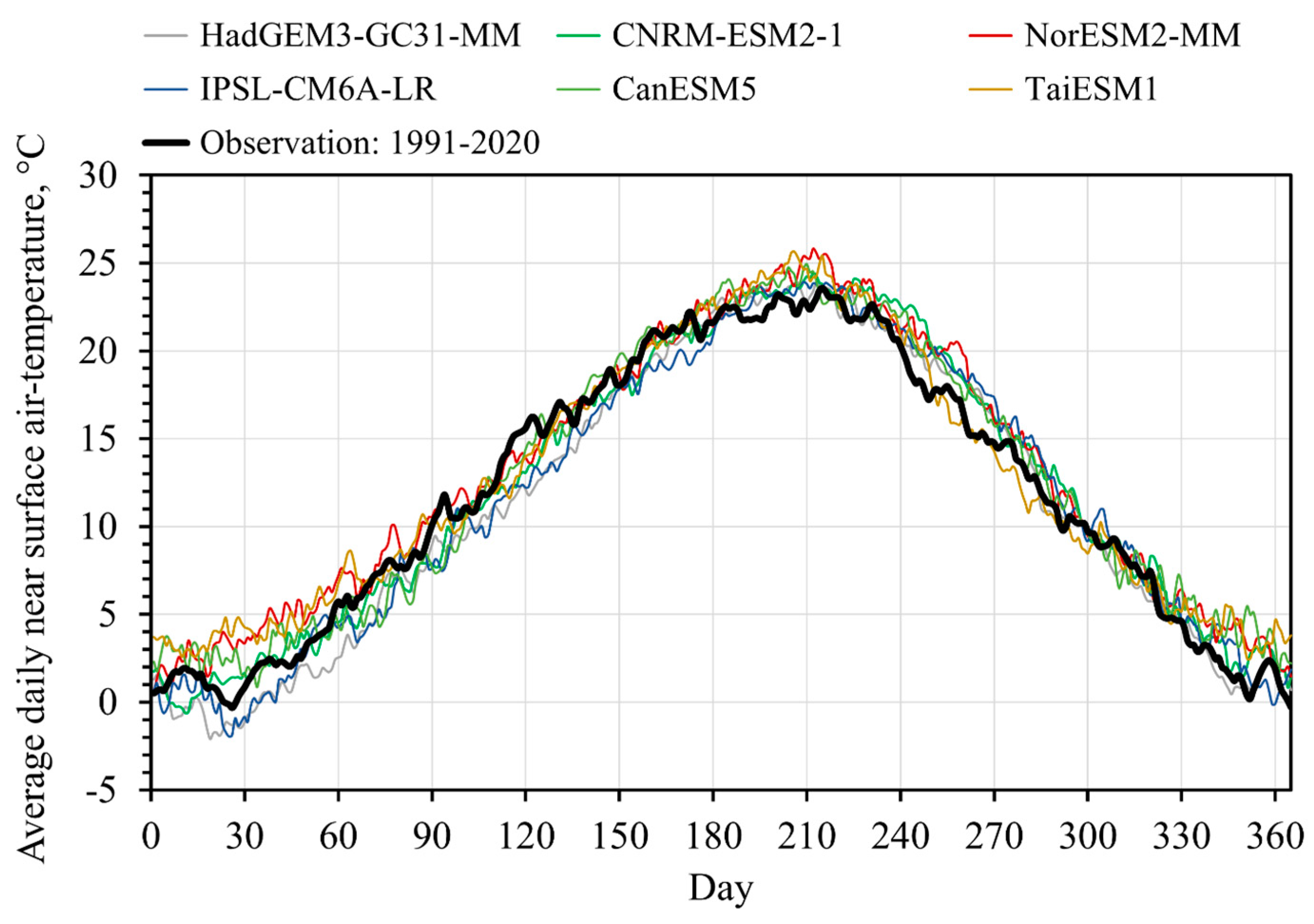
3.1. Comparison between Observed and Predicted Air Temperatures

The Climate Data Store comprises 27 climate models within the CMIP6 framework that are capable of generating historical (1850–2014) and future (2015–2100) climate data on a 1-day time basis. Historical simulations are performed using observed data for atmospheric composition, radiative forcing, and land use while initial conditions are obtained from pre-industrial control simulations. Future climate simulations assume shared socioeconomic pathways (SSP) to derive the greenhouse gas emissions, atmospheric compositions, and radiative forcings necessary for running general circulation models (GCM) into the future. Two representative SSPs are considered, namely the intermediate (SSP2-4.5) scenario and the extreme (SSP5-8.5) scenario. The intermediate climate-change scenario (SSP2-4.5) uses a radiative forcing of 4.5 W/m² and predicts a gradual shift towards sustainability. In this scenario, greenhouse gas emissions remain constant around present levels before starting to fall after mid-century but do not reach net zero by 2100. Average global temperatures are 2.7 °C higher by the end of the century. The extreme climate-change scenario (SSP5-8.5) uses a radiative forcing of 8.5 W/m² and represents a future with energy-intensive economies still based on fossil fuels. Greenhouse gas emissions continue to increase and, by 2050, are about twice as high as present-day levels. Average global temperatures rise 4.4 °C by the end of the century, a future to be avoided at all costs.

Geothermal power depends mainly on the conditions beneath the Earth’s surface, which are usually stable. However, extreme weather events, such as prolonged droughts and intense storms, could also pose an increasing risk in the future. Prolonged droughts could reduce groundwater levels, causing reduced electricity generation from geothermal units. Intense storms could damage the electricity generation and transmission infrastructure, leading to more frequent power outages.

Figure 3 shows the comparison between the observed and predicted daily average air temperatures over the period 1991–2020. Out of the 27 analyzed climate models, the best 6 models are included in Figure 3. The results comprise historical simulations for 1991–2014 and future simulations based on the SSP5-8.5 scenario for 2015–2020. The climate models are ranked by their respective RMSE and KL ranks. For instance, the HadGEM3-GC31-MM climate model achieves an RMSE value of 1.529 °C, ranking it second after the CNRM-ESM2-1 with an RMSE value of 1.377 °C, which is first. However, the former climate achieves a KL value of 0.256, ranking it in the third place, while the latter achieves a KL value of 0.283, ranking it fifth. Then, the overall rank of a climate model is calculated as the average rank score of the RMSE rank and KL rank. The HadGEM3-GC31-MM climate model is ranked first overall, with an average rank value of 2.5, while the CNRM-ESM2-1 climate model is ranked second overall, with an average rank value of 3.0. The ranks and scores of the climate models are listed in

Table 1. Prediction performance of CMIP6 climate models against observed data.

Climate Model	RMSE, °C	KL, -	RMSE Rank	KL Rank	Average Rank Score	Overall Rank
HadGEM3-GC31-MM	1.529	0.256	2	3	2.5	1
CNRM-ESM2-1	1.377	0.283	1	5	3.0	2
NorESM2-MM	1.627	0.280	5	4	4.5	3
IPSL-CM6A-LR	1.566	0.351	4	9	6.5	4
CanESM5	1.551	0.444	3	13	8.0	5
TaiESM1	1.629	0.371	6	10	8.0	5
CESM2-WACCM	1.894	0.256	15	2	8.5	7
HadGEM3-GC31-LL	2.243	0.249	16	1	8.5	7
CNRM-CM6-1	1.683	0.323	11	7	9.0	9
CNRM-CM6-1-HR	1.647	0.421	9	11	10.0	10
CMCC-ESM2	1.643	0.446	7	15	11.0	11
MRI-ESM2-0	1.858	0.344	14	8	11.0	11
MIROC6	1.664	0.487	10	17	13.5	13
EC-Earth3-CC	1.645	0.544	8	19	13.5	13
CMCC-CM2-SR5	2.319	0.439	17	12	14.5	15

.

Multiple climate models can be combined together into ensembles, which are expected to perform better than individual climate models. In the present study, the multi-model ensemble is built using the six best-performing climate models. Figure 4 compares the multi-model prediction (blue lines) with the observed temperature data (black lines). Data dispersion is represented by two standard deviations around the mean (±2 sigma), which encompass 95.45% of the data under the normality assumption. Relative to the individual climate models, the multi-model ensemble increases the prediction accuracy. The RMSE of the multi-model is 1.130 °C, while the average RMSE of the top-six climate models is 1.547 °C.

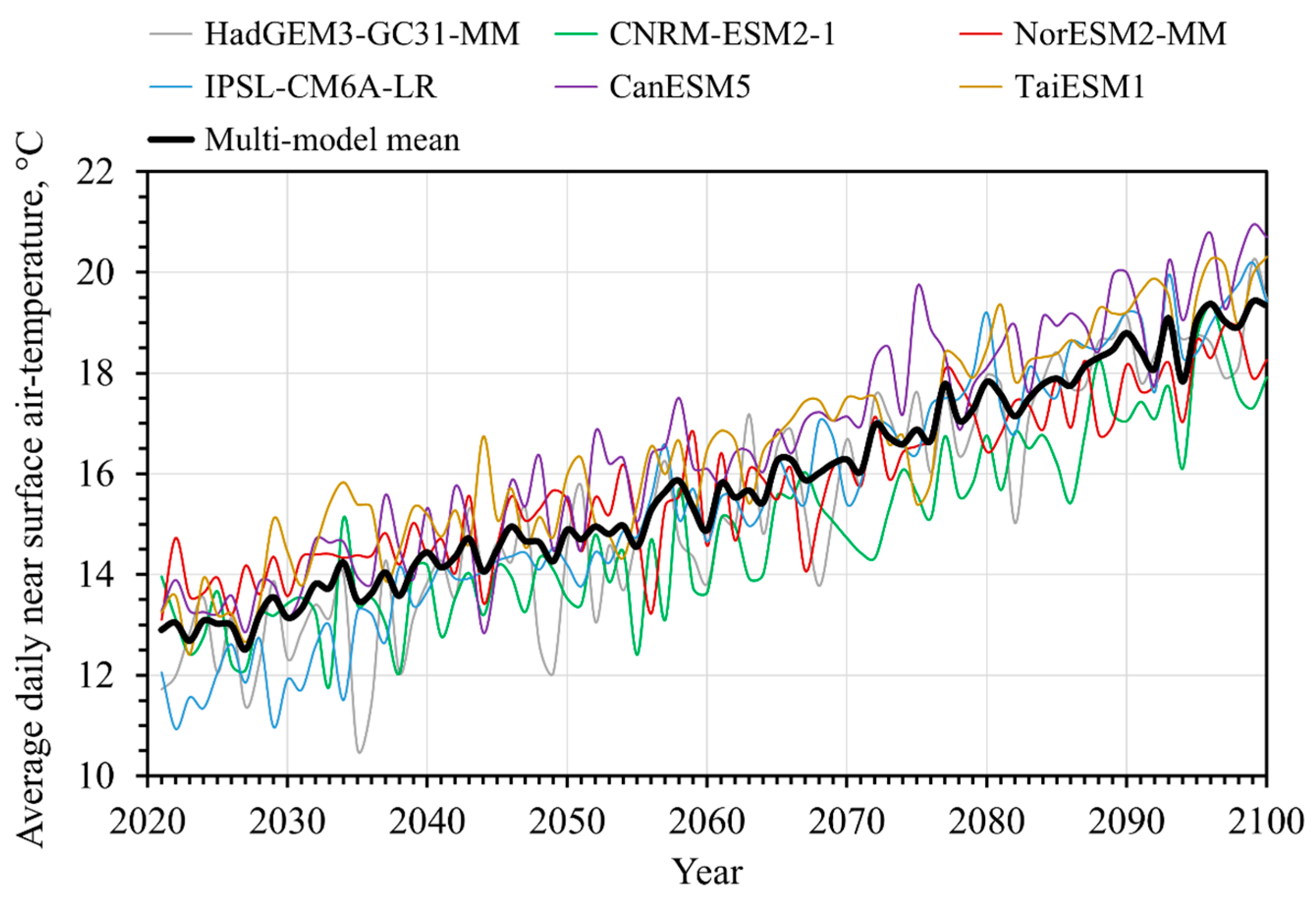
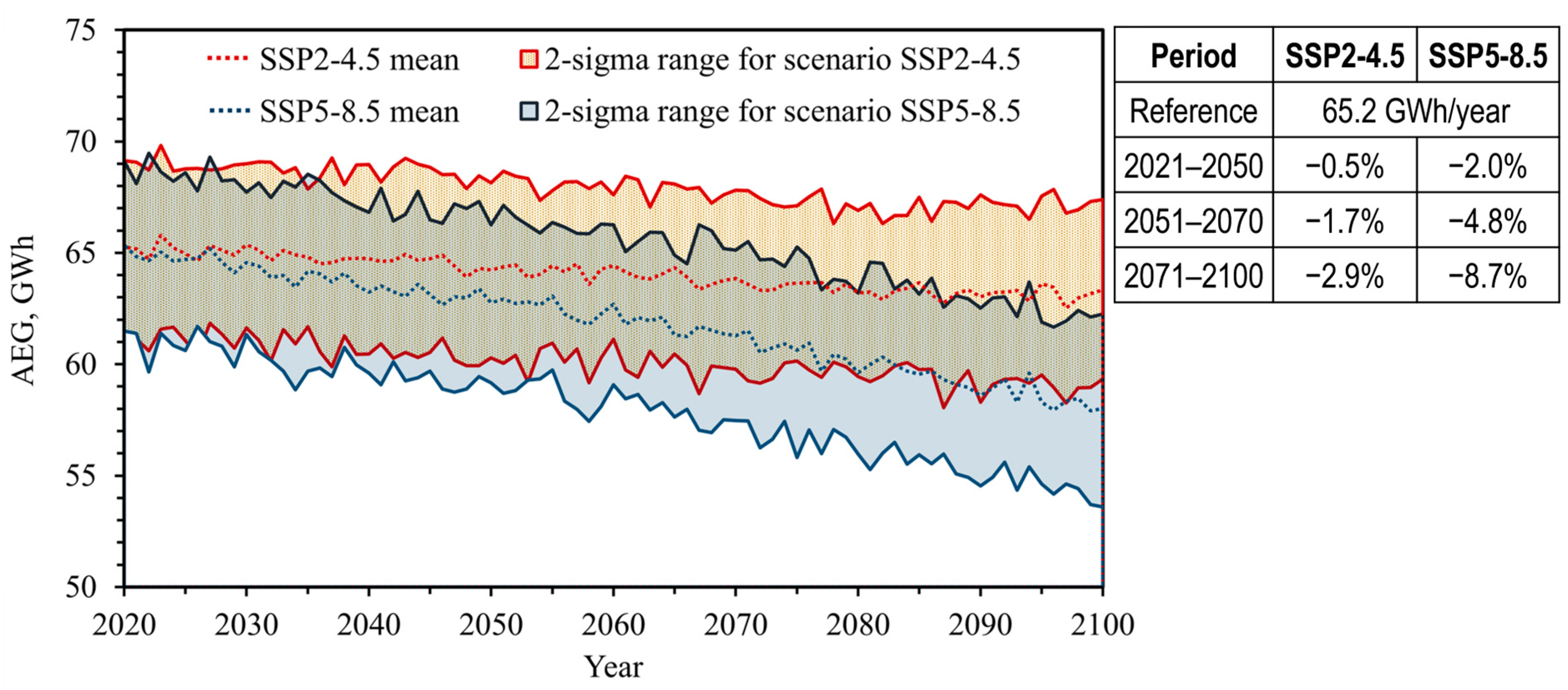
3.2. Future Thermoeconomic Performance of the Geothermal Power Plant

Figure 5 shows the average annual air temperature in Bjelovar under the extreme SSP5-8.5 scenario, as predicted by the top-six climate models and their multi-model mean. In the extreme scenario, the average annual air temperature increases from 12.0 °C in the reference period (1991–2020) up to 18.8 °C in the last decade (2091–2100) of the 21st century. The temperature rise of 6.8 °C in Bjelovar is comparable to the 6.2 °C temperature anomaly predicted by the IPCC AR6 for Croatia [36]. The intermediate (SSP2-4.5) scenario is more moderate. The temperature increase is 3.6 °C in the present analysis and 3.7 °C in the IPCC AR6 for Croatia [36].

Figure 6 shows the temperature-entropy chart of the single-stage ORC configuration (Figure 1). For an ambient air temperature of 12 °C, which is the average for 1991–2020 in Bjelovar, a geothermal fluid inlet temperature of 160 °C, and a mass flow rate of 225 kg/s (810 t/h), the gross and the net powers are 12.2 MW and 10 MW, respectively. The gross and the net thermal efficiencies of the single-stage ORC configuration are 14.3% and 11.6%, respectively. The LCOE is 79.2 USD/MWh and the SIC is 5400 USD/kW.

All simulation runs assume a dry saturated state at the turbine inlet. Cycle optimization is performed for all simulation runs to maximize heat extraction from the geothermal fluid. This involves searching for a turbine inlet pressure p₁ that leads to the optimum thermal match between the geothermal fluid and the isobutane, which is determined with a pinch-point temperature of T₁₀ − T₈ = 10 °C and a reinjection temperature of T₁₁ = 70 °C. For the cycle in Figure 6, this is obtained with p₁ = 23.5 bar (T₁ = 109.2 °C).

Figure 7 and Figure 8 show the annual electricity generation (AEG) and the LCOE in the observed geothermal power plant, as predicted by the multi-model mean, along with the two-sigma ranges (95.45% interval certainty). The analysis involves short-term (2021–2050), medium-term (2051–2070), and long-term (2071–2100) projections. The AEG of geothermal power is expected to decline between 0.5% and 2.9% in the intermediate climate-change scenario (SSP2-4.5) and between 2.0% and 8.7% in the extreme scenario (SSP5-8.5). The LCOE will increase between 0.4% and 1.8% in the intermediate scenario and from 1.3% to 5.6% in the extreme scenario.

4. Conclusions

The ambient air temperature affects the performance of the geothermal power plant by acting on the operating conditions in the ACC. A higher ambient temperature increases the saturation temperature in the ACC and reduces the available enthalpy difference between the turbine and the condenser. Consequently, the power output, electricity generation, and cost metrics, such as LCOE and SIC, are affected.

The present study focuses on long-term temperature variations over the period between 2021 and 2100. It was found that the extreme climate-change scenario (SSP5-8.5) would produce a significant impact on the geothermal power-plant performance by reducing the average AEG by 4.8% in the medium term (2051–2070) and by 8.7% in the long term (2071–2100). Concerning the LCOE, the extreme climate-change scenario predicts an average annual increase of 3.0% in the medium term and 5.6% in the long term. The predictions of the intermediate scenario (SSP2-4.5) are less worrying. The reduction of AEG is 2.9%, while the increase of LCOE is 1.8%, as predicted for the long term.

Future research should attempt to expand the analysis onto different ORC configurations and other working fluids and mixtures and include more climate data for different geographical locations. Also, another interesting line of research could address shorter time scales, such as daily, monthly, and seasonal temperature variations in the analysis of the impact of climate change on the performance of geothermal power plants.

References

1. Sanyal, S.K.; Enedy, S.K. Fifty Years of Power Generation at the Geysers Geothermal Field, California—The Lessons Learned. In Proceeding of the 36th Workshop on Geothermal Reservoir Engineering, Stanford University, Stanford, CA, USA, 31 January–2 February 2011. [Google Scholar]
2. EIA: Electricity Data Browser, Number of Geothermal Power Plants, USA. Available online: https://www.eia.gov/electricity/data/browser/#/topic/1?agg=2,0,1&fuel=001&geo=g&sec=g&freq=A&rtype=s&start=2001&end=2023&ctype=linechart&ltype=pin&rse=0&pin=&maptype=0 (accessed on 1 June 2024).
3. Fridriksson, T.; Merino, A.M.; Orucu, A.Y.; Audinet, P. Greenhouse Gas Emissions from Geothermal Power Production. In Proceedings of the 42nd Workshop on Geothermal Reservoir Engineering, Stanford University, Stanford, CA, USA, 13–15 February 2017. [Google Scholar]
4. New Zealand Geothermal Association: Geothermal Emissions in New Zealand. Available online: https://www.nzgeothermal.org.nz/geothermal-in-nz/what-is-geothermal/ (accessed on 1 June 2024).
5. IPCC. Special Report on Renewable Energy Sources and Climate Change Mitigation; Cambridge University Press: Cambridge, UK; New York, NY, USA, 2011; Available online: https://www.ipcc.ch/site/assets/uploads/2018/03/SRREN_Full_Report-1.pdf (accessed on 1 June 2024).
6. da Silva, B.C.; Virgílio, R.M.; Nogueira, L.A.H.; Silva, P.d.N.; Passos, F.O.; Welerson, C.C. Assessment of Climate Change Impact on Hydropower Generation: A Case Study for Três Marias Power Plant in Brazil. Climate 2023, 11, 201. [Google Scholar] [CrossRef]
7. Dallison, R.J.H.; Patil, S.D. Impact of Climate Change on Hydropower Potential in the UK and Ireland. Renew. Energy 2023, 207, 611–628. [Google Scholar] [CrossRef]
8. Kara, T.; Şahin, A.D. Implications of Climate Change on Wind Energy Potential. Sustainability 2023, 15, 14822. [Google Scholar] [CrossRef]
9. Bonanno, R.; Viterbo, F.; Maurizio, R.G. Climate Change Impacts on Wind Power Generation for the Italian Peninsula. Reg. Environ. Chang. 2023, 23, 15. [Google Scholar] [CrossRef]
10. Solaun, K.; Cerdá, E. Climate Change Impacts on Renewable Energy Generation. A Review of Quantitative Projections. Renew. Sustain. Energy Rev. 2019, 116, 109415. [Google Scholar] [CrossRef]
11. van Vliet, M.T.H.; Wiberg, D.; Leduc, S.; Riahi, K. Power Generation System Vulnerability and Adaptation to Changes in Climate and Water Resources. Nat. Clim. Chang. 2016, 6, 375–380. [Google Scholar] [CrossRef]
12. Georgopoulou, E.; Mirasgedis, S.; Sarafidis, Y.; Giannakopoulos, C.; Varotsos, K.V.; Gakis, N. Climate Change Impacts on the Energy System of a Climate-Vulnerable Mediterranean Country (Greece). Atmosphere 2024, 15, 286. [Google Scholar] [CrossRef]
13. Congedo, P.M.; Baglivo, C.; D’Agostino, D.; Mazzeo, D. The Impact of Climate Change on Air Source Heat Pumps. Energy Convers. Manag. 2023, 276, 116554. [Google Scholar] [CrossRef]
14. Mideksa, T.K.; Kallbekken, S. The Impact of Climate Change on the Electricity Market: A Review. Energy Policy 2010, 38, 3579–3585. [Google Scholar] [CrossRef]
15. Osman, A.I.; Chen, L.; Yang, M.; Msigwa, G.; Farghali, M.; Fawzy, S.; Rooney, D.W.; Yap, P.S. Cost, Environmental Impact, and Resilience of Renewable Energy under a Changing Climate: A Review. Environ. Chem. Lett. 2022, 21, 741–764. [Google Scholar] [CrossRef]
16. Girgibo, N.; Hiltunen, E.; Lü, X.; Mäkiranta, A.; Tuomi, V. Risks of Climate Change Effects on Renewable Energy Resources and the Effects of their Utilisation on the Environment. Energy Rep. 2024, 11, 1517–1534. [Google Scholar] [CrossRef]
17. Linnerud, K.; Mideksa, T.K.; Eskeland, G.S. The Impact of Climate Change on Nuclear Power Supply. Energy J. 2011, 32, 149–168. [Google Scholar] [CrossRef]
18. Petrakopoulou, F.; Robinson, A.; Olmeda-Delgado, M. Impact of Climate Change on Fossil Fuel Power-Plant Efficiency and Water Use. J. Clean. Prod. 2020, 273, 122816. [Google Scholar] [CrossRef]
19. Canales, F.A.; Jadwiszczak, P.; Jurasz, J.; Wdowikowski, M.; Ciapała, B.; Kaźmierczak, B. The Impact of Long-term Changes in Air Temperature on Renewable Energy in Poland. Sci. Total Environ. 2020, 729, 138965. [Google Scholar] [CrossRef] [PubMed]
20. Yu, F.W.; Chan, K.T.; Sit, R.K.Y.; Yang, J. Energy Simulation of Sustainable Air-cooled Chiller System for Commercial Buildings under Climate Change. Energy Build. 2013, 64, 162–171. [Google Scholar] [CrossRef]
21. Ma-oon, K. Geothermal Power Plant Project Ijen Bondowoso: Climate Change Risk Assessment, MedcoEnergi Geothermal, Project 0694710, Bangkok, Thailand. 2023. Available online: https://www3.dfc.gov/environment/eia/ijen/Climate_Change_Risk_Assessment.pdf (accessed on 1 June 2024).
22. Algieri, A. Energy Exploitation of High-Temperature Geothermal Sources in Volcanic Areas: A Possible ORC Application in Phlegraean Fields (Southern Italy). Energies 2018, 11, 618. [Google Scholar] [CrossRef]
23. Vanslambrouck, B.; Vankeirsbilck, I.; van den Broek, M.; Gusev, S.; De Paepe, M. Efficiency Comparison between the Steam Cycle and the Organic Rankine Cycle for Small Scale Power Generation. In Proceedings of the Renewable Energy World Conference & Expo North America, Long Beach, CA, USA, 14–16 February 2012. [Google Scholar]
24. EVAPCO: Eco-Air: Industrial Air-Cooled Condensers. 2020. Bulletin 1100B, 2M/3-19/DGD. Available online: https://www.evapco.com/sites/evapco.com/files/2019-04/eco-Air-Condensers-Brochure-1100B-4.2.2019-web.pdf (accessed on 1 June 2024).
25. Wang, C.-C.; Chi, K.-Y. Heat Transfer and Friction Characteristics of Plain Fin-and-Tube Heat Exchangers, Part I: New Experimental Data. Int. J. Heat Mass Transf. 2000, 43, 2681–2691. [Google Scholar] [CrossRef]
26. Wang, C.-C.; Chi, K.-Y.; Chang, C.-J. Heat Transfer and Friction Characteristics of Plain Fin-and-Tube Heat Exchangers, Part II: Correlation. Int. J. Heat Mass Transf. 2000, 43, 2693–2700. [Google Scholar] [CrossRef]
27. Shah, R.K.; Sekulić, D.P. Fundamentals of Heat Exchanger Design; John Wiley and Sons, Inc.: Hoboken, NJ, USA, 2003. [Google Scholar]
28. Dobson, M.K.; Chato, J.C. Condensation in Smooth Horizontal Tubes. ASME J. Heat Mass Transf. 1998, 120, 193–213. [Google Scholar] [CrossRef]
29. Collier, J.G.; Thome, J.R. Convective Boiling and Condensation, 3rd ed.; Oxford Engineering Science Series: Oxford, UK, 1996. [Google Scholar]
30. Yunus, A.C.; Afshin, J.G. Heat and Mass Transfer: Fundamentals and Applications, 6th ed.; McGraw-Hill Education: New York, NY, USA, 2020. [Google Scholar]
31. Serth, R.W.; Lestina, T. Process Heat Transfer: Principles, Applications and Rules of Thumb, 2nd ed.; Academic Press: Cambridge, MA, USA, 2014. [Google Scholar]
32. Intergovernmental Panel for Climate Change (IPCC): Sixth Assessment Report (AR6). 2021. Available online: https://www.ipcc.ch/assessment-report/ar6/ (accessed on 1 June 2024).
33. Copernicus Climate Change Service, Climate Data Store (CDS): CMIP6 Climate Projections. 2021. Available online: https://cds.climate.copernicus.eu/cdsapp#!/dataset/10.24381/cds.c866074c?tab=overview (accessed on 1 June 2024).
34. Croatian Meteorological and Hydrological Service (DHMZ): Climate—Daily Mean Temperature. Available online: https://meteo.hr/klima_e.php?section=klima_pracenje&param=srednja_temperatura (accessed on 1 June 2024).
35. Weiss, A.; Hays, C.J. Calculating Daily Mean Air Temperatures by Different Methods: Implications from a Non-Linear Algorithm. Agric. For. Meteorol. 2005, 128, 57–65. [Google Scholar] [CrossRef]
36. Climate Change Knowledge Portal: Climate Projections—Mean Projections, Country: Croatia. Available online: https://climateknowledgeportal.worldbank.org/country/croatia/climate-data-projections (accessed on 1 June 2024).
Figure 1. The single-stage configuration of the ORC geothermal power plant.
Engproc 67 00029 g001
Figure 2. The air-cooled condenser (ACC).
Engproc 67 00029 g002
Figure 3. Daily average near-surface air temperature in Bjelovar, Croatia (45.8988° N, 16.8423° E) for the reference period of 1991–2020: A comparison between observations and predictions of CMIP6 climate models.
Engproc 67 00029 g003
Figure 4. Daily average near-surface air temperature in Bjelovar, Croatia (45.8988° N, 16.8423° E) for the reference period of 1991–2020: A comparison between observations and CMIP6 multi-model predictions.
Engproc 67 00029 g004
Figure 5. Average annual near-surface air temperature in Bjelovar (45.8988° N, 16.8423° E) from 2021 to 2100, under the extreme climate-change scenario (SSP5-8.5).
Engproc 67 00029 g005
Figure 6. T-s chart of the single-stage ORC configuration with isobutane as working fluid. For the meaning of line colors and point states refer to Figure 1.
Engproc 67 00029 g006
Figure 7. Impact of climate change on the AEG of the single-stage ORC geothermal power plant.
Engproc 67 00029 g007
Figure 8. Impact of climate change on the LCOE of the single-stage ORC geothermal power plant.
Engproc 67 00029 g008