Abstract
Synthetic time series generation is an emerging field of study in the broad spectrum of data science, addressing critical needs in diverse fields such as finance, meteorology, and healthcare. In recent years, diffusion methods have shown impressive results for image synthesis thanks to models such as Stable Diffusion and DALL·E, defining the new state-of-the-art methods. In time series generation, their potential exists but remains largely unexplored. In this work, we demonstrate the applicability and suitability of diffusion methods for time series generation on several datasets with a rigorous evaluation procedure. Our proposal, inspired from an existing diffusion model, obtained a better performance than a reference model based on generative adversarial networks (GANs). We also propose a modification of the model to allow for guiding the generation with respect to conditioning variables. This conditioned generation is successfully demonstrated on meteorological data.
1. Introduction
In data science, time series data are particularly widespread and play a crucial role in a variety of fields, such as finance, meteorology, and health. Their analysis underpins various applications, including forecasting, data imputation, and anomaly detection. The generation of synthetic time series is a relatively new subject, but one that is gaining growing interest in the community of generative artificial intelligence. Indeed, time series generation finds several applications such as pre-training machine learning models, testing deployed data pipelines, and graphical illustrations [1]. The pre-training use case is particularly important when there are a lack of real data, when the data are of poor quality, or in case of data confidentiality.
In the field of image synthesis, diffusion methods have already proven their worth and are now considered state-of-the-art methods. Examples include Stable Diffusion [2], DALLE·3 [3], and Midjourney [4], all of which are based on diffusion methods conditioned by textual description to generate realistic, high-quality synthetic images. Diffusion methods have been successfully applied to time series, but their applications are mainly limited to imputation and forecasting tasks and do not include the conditioning aspect [5]. To our knowledge, the generation of synthetic time series using diffusion methods and including conditioning remains under-explored, yet possesses promising potential.
Diffusion methods involve gradually perturbing data with noise until they have completely lost their initial structure, and then gradually denoising them to recover the original data. Respectively, these two processes are called the forward process and the backward process. The backward process is learned by a neural network, which, once trained, is able to generate new synthetic data.
Our work aims to study the suitability and applicability of diffusion methods to the generation of time series. The goal is to create a generative time series model, based on the diffusion principle, which can be conditioned on additional information, and to discuss this performance using an adequate evaluation procedure. More specifically, this work aims to answer the following three research questions (RQs):
- RQ1. Are diffusion methods suitable for generating synthetic time series?
- RQ2. How can we evaluate the quality of the generated time series?
- RQ3. Can the generation of time series be conditioned without degrading the quality of the generated time series?
In the following, we present our methodology and main results that are split into three different experiments. Finally, the results obtained are presented and discussed.
2. Materials and Methods
2.1. Selected Models
Different approaches can be used for time series generation. The TimeGAN model, based on a generative adversarial network, is well established in the state-of-the-art [6], and therefore, we selected it as baseline for our experiments on unconditioned generation.
Other models also use diffusion for tasks such as forecasting, imputation, and generation, for instance, TimeDiff from Shen and Kwok, SSSD from Alcaraz and Strodthoff, or Guided-DiffTime from Coletta et al., all of which have been compared in a recent review by Lin et al. [7,8,9,10].
To our knowledge, the TSDiff model introduced by Biloš et al. is the only work based on a diffusion model for time series generation where its source code has been published [11]. We are also able to envision how to modify the proposed TSDiff architecture to allow for the injection of conditioning. For these reasons, we selected TSDiff for our experiments with the objective to benchmark it against TimeGAN for unconditional generation and to adapt it for conditional generation. We also designed pipelines for reproducible experimentation using diverse evaluation metrics and datasets. Figure 1 and Figure 2 present the pipelines for the training and evaluation of the generators, respectively, for unconditioned and conditioned generation.
2.2. Datasets
We used several datasets to evaluate the generation capabilities on different time series characteristics.
- Stocks: This first dataset contains Google share prices from 2004 to 2019. Due to its nature, these data fluctuate widely and are therefore aperiodic. The data consist of six correlated features, such as volume or opening and closing prices [12].
- Energy: The UCI Appliances energy prediction dataset contains data recorded by several sensors in a house, over a period of four and a half months. These data are characterized by higher dimensionality, somewhat noisy periodicity, and correlated characteristics such as temperature and humidity in different rooms [13].
- MeteoSwiss: This last dataset contains real meteorological data recorded from 2020 to 2022, by 33 weather stations in Switzerland, that have been collected through the IDAweb portal provided by MeteoSwiss [14]. These periodic data contain nine correlated characteristics, such as temperature, atmospheric pressure, and humidity. This dataset is particularly important in this study as it is accompanied by metadata describing the location of weather stations for the conditional generation experiments to be carried out.
- Sine: Finally, we also generated synthetic multivariate sinusoidal time sequences of a certain length to evaluate the performance of our model on periodic data, where each feature is independent of the others.

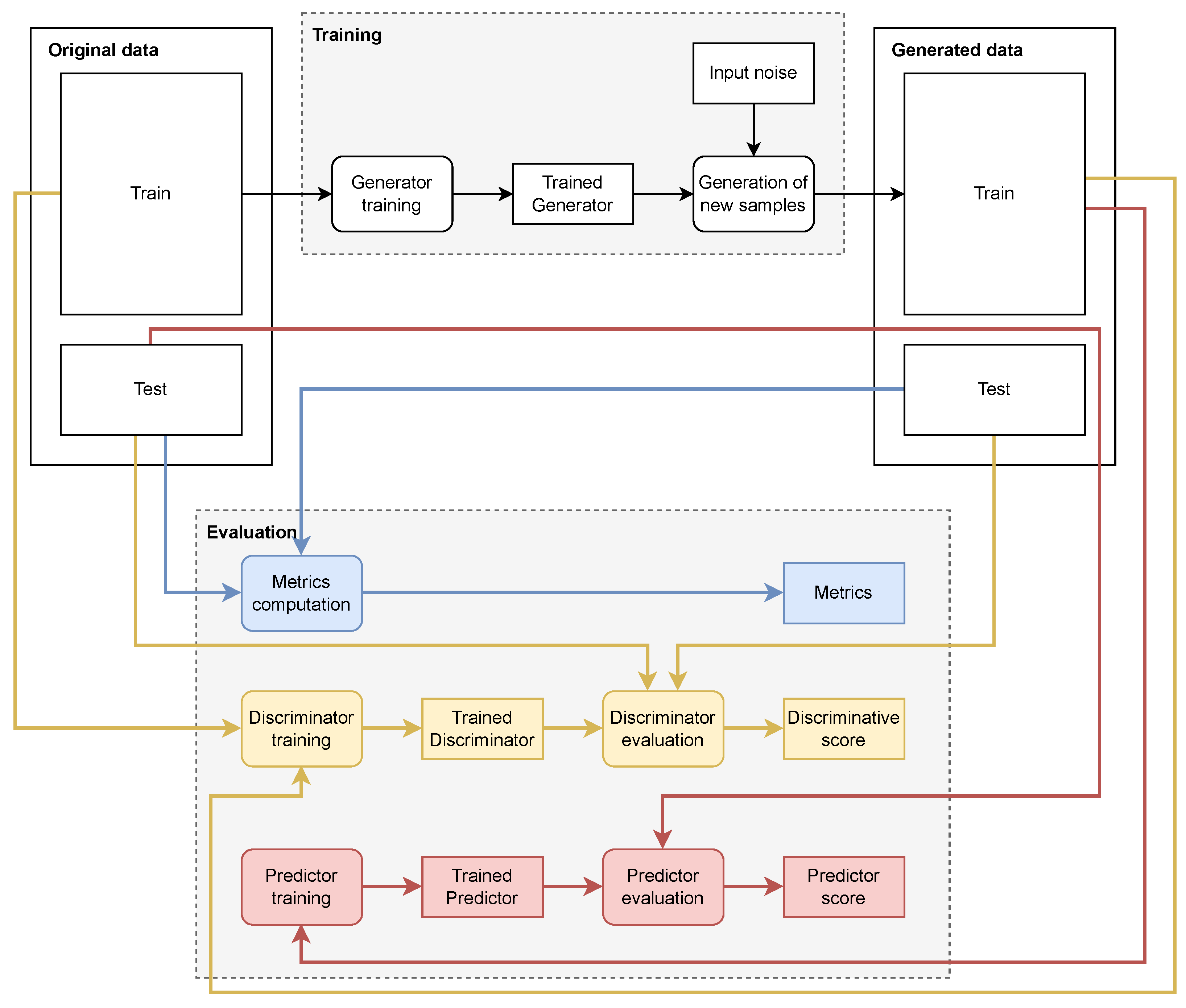
Figure 1.
Data pipelines for unconditional generation, where squared blocks represent train/test/ generated data, models, or scores, and rounded blocks represent processes. The pipeline to train and use the generator is illustrated on the top (white), while the pipelines for evaluation are on the bottom (yellow for DS and red for PS).
2.3. Evaluation Procedures
The evaluation of the quality of a generated time series, especially when they are multivariate, is not as straightforward for a human as its equivalent for a generated image. To cope with this difficulty, different methods are typically used, including visual, statistical, and model-based.
For the visual representation of the generated time series, PCA and t-SNE projections are usually used. They allow us to project high-dimensional generated samples on 2D plots. Such projections provide a qualitative assessment, mostly useful during model development.
Regarding statistical evaluation, the Mean Distribution Difference (MDD) and Auto-correlation Difference (ACD) are typically used. The MDD assesses how closely the distributions of the real and generated data are. The ACD measures how well the generation model has captured the temporal dependencies of the data.
Model-based methods aim at computing quantitative metrics to benchmark the quality of the generation. We opted for the following:
- Discriminative Score (DS): The principle is to train a classifier to discriminate between true and generated samples. A perfect generation model would produce signals that are indistinguishable from the true one, leading to a discriminative score of around 0.5.
- Predictive Score (PS): This method involves the training of a regression model using the generated data. The model is then tested on a predictive task using real data as input. A good regression score (, , etc.) means that the generative model was able to capture and reproduce the characteristics of the time series to allow for the training of predictive models in a similar way as if using real data.
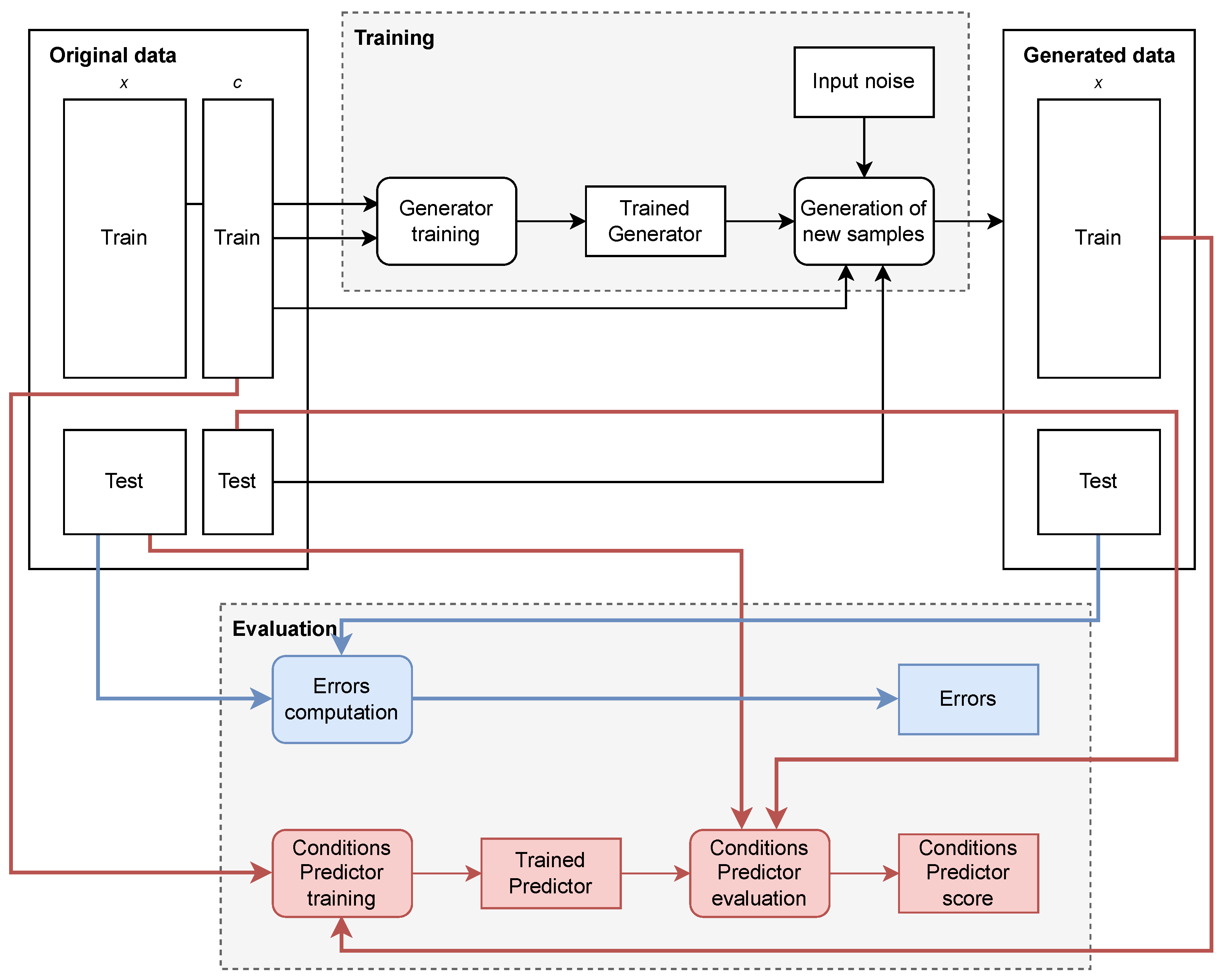
- Conditional Predictive Score (CPS): This method aims at training a model to predict again the conditioning values, taking as input the generated data. A low prediction error indicates that the generated data indeed include features associated to the conditioning. As in the previous method, a “Train on Synthetic, Test on Real” (TSTR) approach is used to train and test the CPS model.
For DS, PS, and CPS, Recurrent Neural Networks composed of two GRU layers were used.

Figure 2.
Data pipelines for conditional generation and evaluation procedures. The conventions are similar as in Figure 1.
Figure 2.
Data pipelines for conditional generation and evaluation procedures. The conventions are similar as in Figure 1.
2.4. Unconditional Generation
We compared the TimeGAN generative adversarial network model [6] and the TSDiff diffusion model [11]. The generation task is here unconditioned, i.e., no further information is injected in the generator. The training and evaluation of TimeGAN and TSDiff are performed on the same datasets, but only with a length of 24 (i.e., one day with one sample per hour), as TimeGAN was designed to handle this length.
The default TimeGAN configuration is used, as described in the original article and in TimeGAN’s Supplementary Materials. Our evaluations are performed by computing the DS, PS, MDD, and ACD, and by visualizing the distribution of the data by projecting them into a two-dimensional space using mainly the t-SNE algorithm.
2.5. Conditional Generation
We modified the architecture of TSDiff to allow for the injection of conditional signals by appending a conditioning vector to the time series in the forward pass of the model.
The ability of the TSDiff model to generate time series conditionally is then evaluated using the MeteoSwiss dataset. We selected this dataset as conditioning variables could easily be crafted for such tasks:
- Statistical Conditioning: Simple statistical properties (mean, std, min, max, median) of the original sequences are used as conditioning variables. Then, an evaluation of the performance of the model on this new created dataset is performed. This showcases the model’s ability to generate sequences conditionally, as generated sequences’ statistics can be directly compared with the ones they were conditioned on (i.e., the original sequences’ statistics).
- Generalized Prediction: The performance on the MeteoSwiss data is evaluated on a random selection of days used for training and testing. The conditioning variables are the longitude, latitude, altitude, and the day of the year. CPS and MAE metrics between generated and ground-truth time series are used to evaluate the performance of the model. This allows us to measure how well the model can “fill in the gaps” when data for some days are not available.
- Station Interpolation: The performance on the MeteoSwiss data is evaluated on stations being specifically selected for training and testing. The conditioning variables are the longitude, latitude, altitude, and the day of the year. The CPS and MAE metrics are used to evaluate the performance of the model. This allows us to measure how well the model can interpolate data for stations that are not available in the training set.
- Future Meteorological Scenarios: The model is trained on MeteoSwiss data of temperature values from a specific station to predict typical days until the year 2050. The conditioning variables used are the day of the year and the year only. This allows us to measure whether the model is capable of modeling global warming with an interesting insight for the future.
The metrics used to evaluate model performance on unconditioned generation are also used to evaluate model performance on conditioned generation. In this way, it ensures that conditioning does not adversely affect model performance.
3. Results
3.1. Unconditional Generation Performance
In this section, the performances of the proposed diffusion model on an unconditional generation task are presented. Table 1 presents the quantitative results on the different datasets. The discriminative and predictor scores (DS and PS) are obtained by training four times the models and averaging the results. The standard deviation of the scores is also reported, thus measuring the variability of the results across the different runs.

Table 1.
Comparison of the results obtained with the diffusion model (TSDiff) and TimeGAN. The best results are in bold.
Overall, the results on real datasets are consistent with the expectations. In particular, the model achieves good results on the Stocks dataset, which is the least complex of the three. It has more difficulty on the Energy dataset, which is characterized by 28 features, particularly in terms of the DS. As the DS on the MeteoSwiss is relatively high as well, it seems more difficult for the model to generate realistic sequences from more complex datasets.
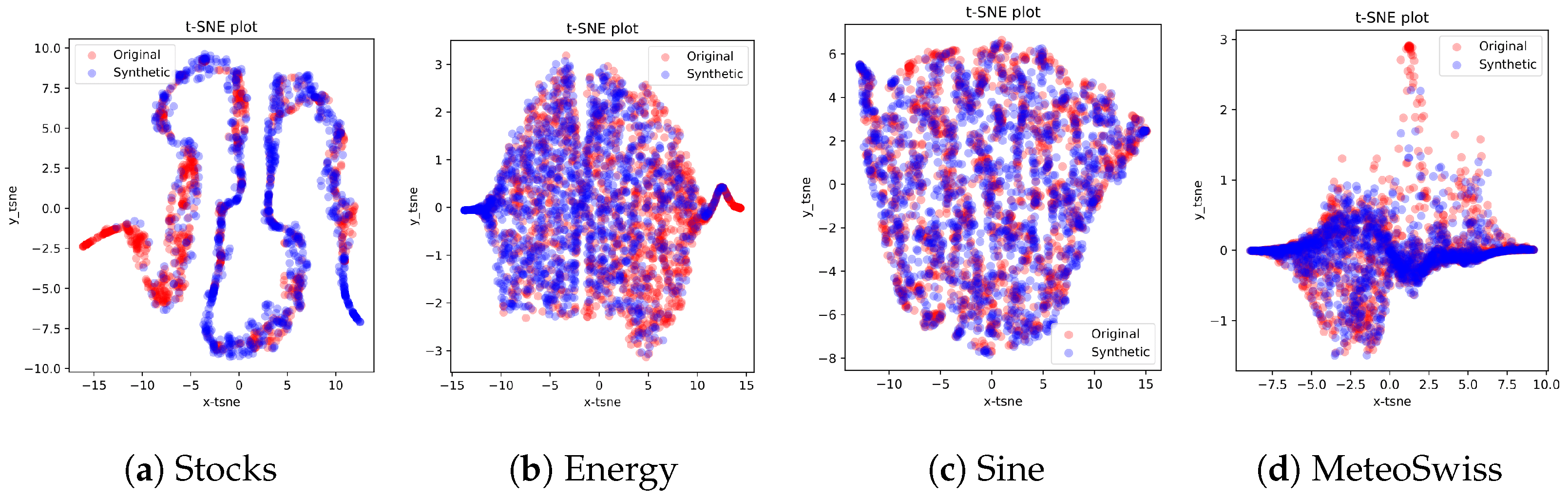
In addition to these quantitative results, Figure 3 presents the t-SNE visualizations for all datasets. These visualizations enable us to compare the distribution of real data with the one generated by the model.
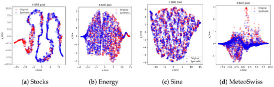
Figure 3.
t-SNE visualizations of the real and generated data for the considered datasets, showing the distribution of the data in a 2D space.
3.2. Conditional Generation
3.2.1. Statistical Conditioning
First, the model performances are evaluated when conditioned on basic statistical properties, using the MeteoSwiss dataset to compare generated sequences against real ones. The model successfully retained the conditioned statistical properties for the most part but struggles with capturing extreme values, particularly minimum and maximum values, indicating a potential limitation in dealing with outliers. Generated sequences closely match real ones in terms of mean values, confirming the model’s efficacy in generating statistically coherent sequences. This assessment reinforces the model’s capability to generate meteorologically relevant sequences based on a variety of conditioning inputs, despite challenges in capturing extremities.
3.2.2. Generalized Prediction
This section evaluates the diffusion model’s ability to generate meteorological sequences with omitted days in the training set, examining its performance through the Conditional Predictive Score (CPS) per variable, as presented in Table 2, and Mean Absolute Error (MAE) across different features, as presented in Table 3.
Table 2.
CPS score for each conditioning variable, obtained by training and evaluating the model on the MeteoSwiss dataset, along with the standard deviation. A lower value is better.
Table 3.
MAE for each feature, obtained by comparing the generated sequences to the real ones on the MeteoSwiss dataset. The sequence length is 24.
The results indicate that while the model effectively generates sequences retaining the conditioning information, it has difficulties regarding the coordinate variables, suggesting that some features influence generation more than others. Errors in sunshine duration suggest a higher challenge in capturing abrupt changes. Also, the model struggles with predicting wind direction components, thus suggesting a limitation in capturing high variability within meteorological sequences.
3.2.3. Station Interpolation
This section discusses the diffusion model’s performance on station interpolation, using data from stations excluded during training. The task proved to be more challenging than generalized prediction as seen on Table 3, with generally increased errors across features.
Interpolation accuracy varied among stations, with noticeable discrepancies in temperature predictions, particularly during warmer months, indicating an overestimation of temperatures by the model. The consistent results across different stations suggest a need for additional conditioning variables to better capture underlying phenomena and improve interpolation accuracy. The overall difficulty emphasizes the complexity of the task rather than the model’s limitations.
3.2.4. Future Meteorological Scenarios
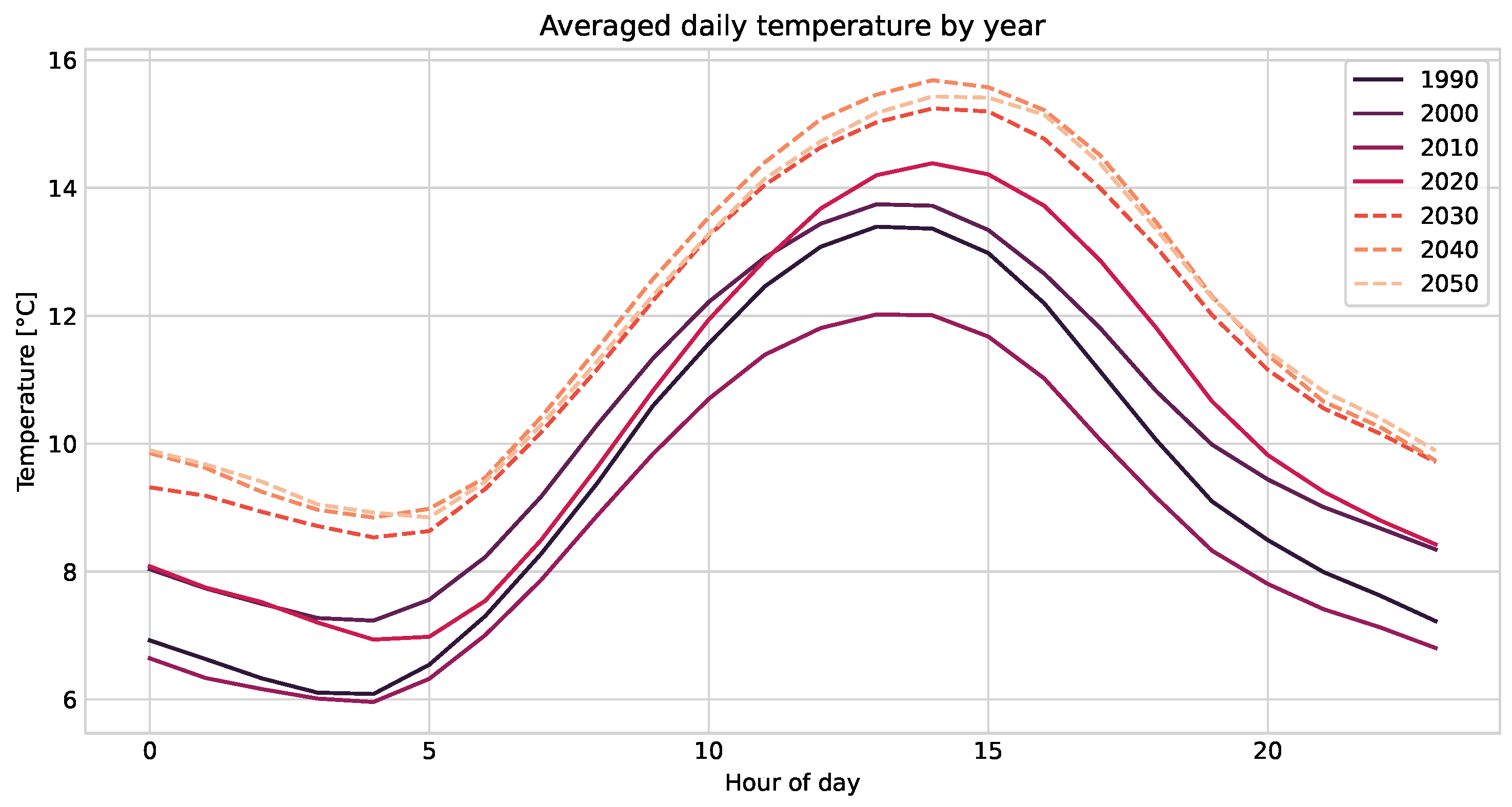
This last experiment gives an insight of the influence of global warming on typical days in Switzerland until 2050. The Figure 4 shows that in terms of temperature, the model predicts increasingly hotter days by 2050. Temperature data from the year 1990 to 2020 are the real values, while those from the year 2030 to 2050 are generated by the model. We can observe that the model has indeed, to some extent, captured the drift of temperature over the years. Here, we need to note that the predicted increase of approximately +1.6 °C on average between 2020 and 2040 is quite large and is therefore more related to an interpolation effect on past data than from any underlying physical model. Although the generation in this experiment should certainly take other phenomena into account, it shows that the diffusion model can be used as a kind of forecaster by conditioning it on temporal data.
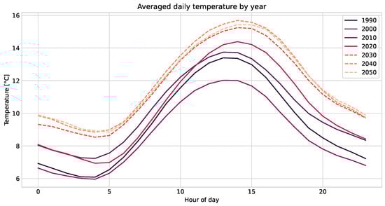
Figure 4.
Averaged daily temperature in Bern (Switzerland) until the year 2050. Solid lines are ground-truth values, while dashed lines are data generated by the diffusion model.
4. Discussion and Conclusions
The results obtained demonstrate the effectiveness of the modified TSDiff model in generating both unconditioned and conditioned time series, with comprehensive validation through sanity checks, quantitative and qualitative measurements, and comparison with an existing reference method.
Experiments specifically carried out on conditional generation reveal the model’s ability to incorporate specific input conditions into the generated series, although with varying degrees of success in different scenarios. This indicates the influence of task complexity and the importance of relevant conditioning information.
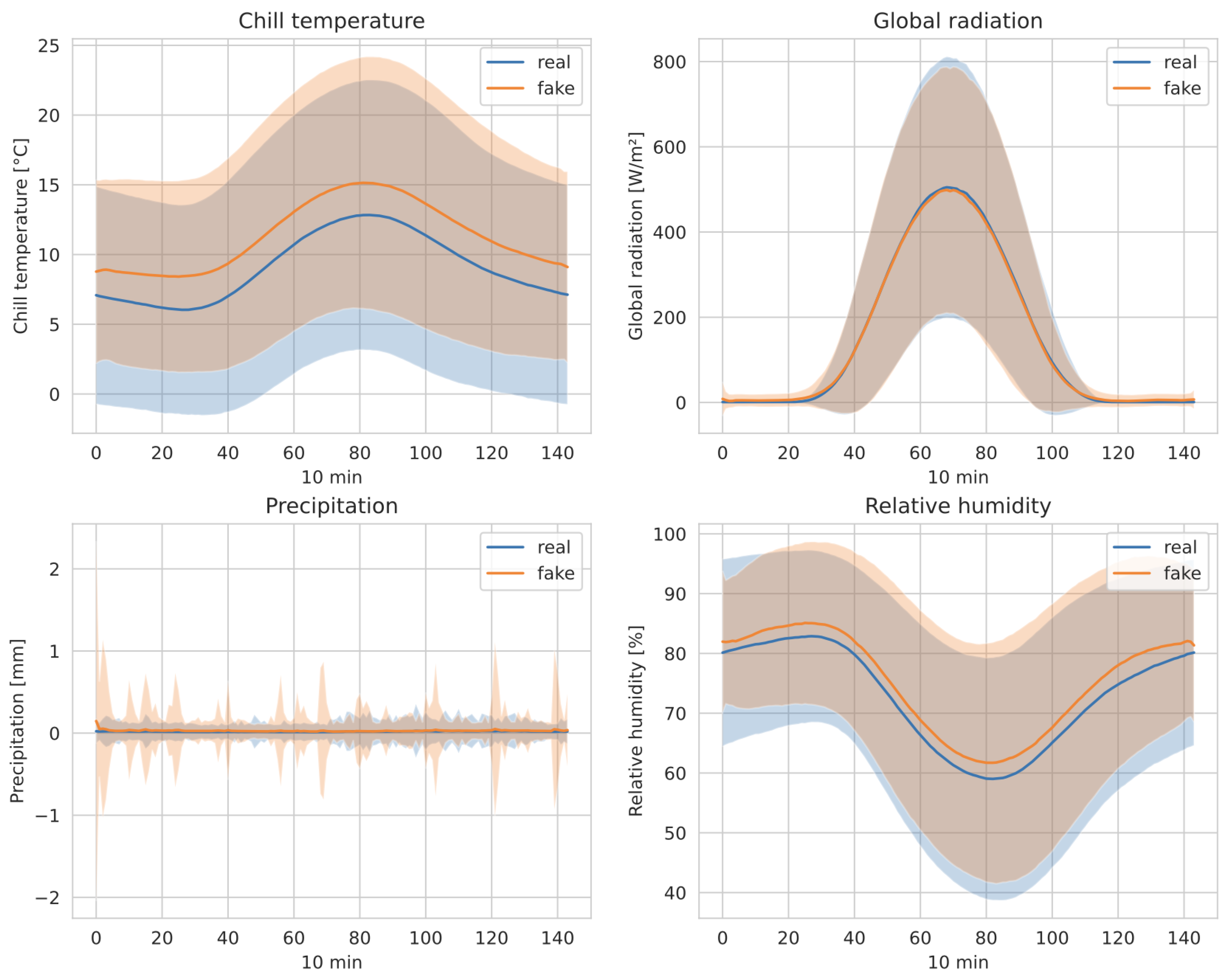
Further analysis highlights the model’s ability to adhere to the statistical properties of the data, with some limitations in capturing extreme values. In this regard, a few examples are plotted in Figure 5. Overall, the results confirm the potential of diffusion models in time series generation, although some improvements should be considered.

Figure 5.
Averaged generated sequences on a selection of features, compared to the real sequences. Standard deviation is represented by the shaded area.
Author Contributions
Conceptualization, B.P., F.M., B.W., and J.H.; methodology, B.P.; software, B.P.; validation, F.M. and J.H.; formal analysis, B.P.; investigation, B.P. and F.M.; resources, J.H. and F.M.; data curation, B.P.; writing—original draft preparation, B.P. and F.M.; writing—review and editing, F.M., B.W. and J.H.; visualization, B.P.; supervision, J.H., B.W. and F.M.; project administration, J.H.; funding acquisition, J.H. All authors have read and agreed to the published version of the manuscript.
Funding
This research is funded through structural funds of the Institute of Artificial Intelligence and Complex Systems—iCoSys at HEIA-FR, HES-SO, Switzerland.
Institutional Review Board Statement
Not applicable.
Informed Consent Statement
Not applicable.
Data Availability Statement
Section 2.2 presents all datasets available in this study. The datasets Stocks and Energy are available in publicly accessible repositories mentioned in the references. The dataset MeteoSwiss is available on request from the authors.
Acknowledgments
The authors would like to thank Beat Schaffner and Mario Rindlisbacher from the company Meteotest AG (https://meteotest.ch, accessed on 1 July 2024 ) for their guidance related to weather data. Also, we would like to thank MeteoSwiss for providing access to their weather data.
Conflicts of Interest
The authors declare no conflicts of interest.
References
- Wen, Q.; Sun, L.; Song, X.; Gao, J.; Wang, X.; Xu, H. Time Series Data Augmentation for Deep Learning: A Survey. arXiv 2020, arXiv:2002.12478. [Google Scholar]
- Rombach, R.; Blattmann, A.; Lorenz, D.; Esser, P.; Ommer, B. High-Resolution Image Synthesis with Latent Diffusion Models. arXiv 2022, arXiv:2112.10752. [Google Scholar] [CrossRef]
- OpenAI. DALL-E 3. 2024. Available online: https://openai.com/dall-e-3 (accessed on 7 February 2024).
- Midjourney. Available online: https://www.midjourney.com/ (accessed on 7 February 2024).
- Kollovieh, M.; Ansari, A.F.; Bohlke-Schneider, M.; Zschiegner, J.; Wang, H.; Wang, Y. Predict, Refine, Synthesize: Self-Guiding Diffusion Models for Probabilistic Time Series Forecasting. arXiv 2023, arXiv:2307.11494. [Google Scholar]
- Yoon, J.; Jarrett, D.; van der Schaar, M. Time-series Generative Adversarial Networks. In Advances in Neural Information Processing Systems; Curran Associates, Inc.: New York, NY, USA, 2019; Volume 32. [Google Scholar]
- Shen, L.; Kwok, J. Non-autoregressive conditional diffusion models for time series prediction. In Proceedings of the International Conference on Machine Learning, Honolulu, HI, USA, 23–29 July 2023; pp. 31016–31029. [Google Scholar]
- Alcaraz, J.M.L.; Strodthoff, N. Diffusion-based Time Series Imputation and Forecasting with Structured State Space Models. arXiv 2023, arXiv:2208.09399. [Google Scholar] [CrossRef]
- Coletta, A.; Gopalakrishnan, S.; Borrajo, D.; Vyetrenko, S. On the Constrained Time-Series Generation Problem. In Advances in Neural Information Processing Systems; Oh, A., Neumann, T., Globerson, A., Saenko, K., Hardt, M., Levine, S., Eds.; Curran Associates, Inc.: New York, NY, USA, 2023; Volume 36, pp. 61048–61059. [Google Scholar]
- Lin, L.; Li, Z.; Li, R.; Li, X.; Gao, J. Diffusion models for time-series applications: A survey. Front. Inf. Technol. Electron. Eng. 2023, 25, 19–41. [Google Scholar] [CrossRef]
- Biloš, M.; Rasul, K.; Schneider, A.; Nevmyvaka, Y.; Günnemann, S. Modeling temporal data as continuous functions with stochastic process diffusion. In Proceedings of the 40th International Conference on Machine Learning, Honolulu, HI, USA, 23–29 July 2023; Volume 202, pp. 2452–2470. [Google Scholar]
- Alphabet Inc. Alphabet Inc. (GOOG) Stock Historical Prices & Data—Yahoo Finance. Available online: https://finance.yahoo.com/quote/GOOG/history/ (accessed on 4 April 2023).
- Candanedo, L. Appliances Energy Prediction. UCI Machine Learning Repository. 2017. Available online: https://doi.org/10.24432/C5VC8G (accessed on 4 July 2024).
- MeteoSwiss. Federal Office of Meteorology and Climatology MeteoSwiss. Available online: https://www.meteoswiss.admin.ch (accessed on 2 February 2023).
Disclaimer/Publisher’s Note: The statements, opinions and data contained in all publications are solely those of the individual author(s) and contributor(s) and not of MDPI and/or the editor(s). MDPI and/or the editor(s) disclaim responsibility for any injury to people or property resulting from any ideas, methods, instructions or products referred to in the content. |
© 2024 by the authors. Licensee MDPI, Basel, Switzerland. This article is an open access article distributed under the terms and conditions of the Creative Commons Attribution (CC BY) license (https://creativecommons.org/licenses/by/4.0/).