Energy Efficiency Evaluation of Frameworks for Algorithms in Time Series Forecasting ^†

Abstract

In this study, the energy efficiency of time series forecasting algorithms is addressed in a broad context, highlighting the importance of optimizing energy consumption in computational applications. The purpose of this study is to compare the energy efficiency and accuracy of algorithms implemented in different frameworks, specifically Darts, TensorFlow, and Prophet, using the ARIMA technique. The experiments were conducted on a local infrastructure. The Python library CodeCarbon and the physical energy consumption measurement device openZmeter were used to measure the energy consumption. The results show significant differences in energy consumption and algorithm accuracy depending on the framework and execution environment. We conclude that it is possible to achieve an optimal balance between energy efficiency and accuracy in time series forecasting, which has important implications for developing more sustainable and efficient applications. This study provides valuable guidance for researchers and professionals interested in the energy efficiency of forecasting algorithms.

1. Introduction

In the digital age, machine learning (ML) has transformed various fields by providing advanced tools for data-driven decision making. Time series forecasting, particularly in finance, healthcare, supply chain management, and energy production, has significantly benefited from these advancements [1]. This capability enables organizations to optimize operations, manage risks, and improve planning accuracy. However, the increasing complexity of these models has led to higher computational demands and energy consumption.

The energy consumption associated with different types of algorithms, particularly in time series forecasting models, is a growing concern from both economic and environmental perspectives [2]. As organizations aim to enhance the accuracy of their models, they often resort to more complex algorithms and more powerful computational infrastructures. This rise in energy demand incurs additional costs and impacts the environment through increased greenhouse gas emissions. In a global context where sustainability and carbon footprint reduction are priorities, assessing the energy efficiency of these models and frameworks is crucial. Moreover, there are time series algorithms specifically designed to measure the energy efficiency of various systems and processes [3], further emphasizing the importance of optimizing energy usage not only in computational tasks but across different sectors.

In this context, the energy efficiency of data processing algorithms has been extensively studied. Merelo-Guervós et al. [4] optimized evolutionary algorithms in the JavaScript language, showing that carefully selecting data structures and eliminating unnecessary memory allocations can significantly reduce energy consumption. On the other hand, Escobar et al. [5] developed a distributed K-nearest neighbors (KNN) algorithm for EEG signal classification by using the minimum redundancy-maximum relevance (mRMR) feature selection technique and an energy policy that adjusts execution based on cost, they improved energy efficiency in heterogeneous clusters.

Furthermore, Díaz et al. [6] created the Vampire system, a low-cost tool for the real-time monitoring of energy consumption in distributed computing systems. Utilizing an ESP32 microcontroller and the MQTT protocol, Vampire efficiently records and analyzes energy consumption in 60-core clusters. Complementing these studies, Prieto et al. compared the energy efficiency of personal computers (PCs) with mainframes and supercomputers, demonstrating that PCs can achieve efficiency levels similar to those of systems in the Green500 ranking. These studies indicate that migrating processes to more energy-efficient resources and implementing energy monitoring and management technologies can significantly reduce the global energy consumption, promoting environmental sustainability [7].

In this research, we conduct a systematic analysis of the energy efficiency of various ML frameworks used for time series forecasting. By comparing statistical techniques such as ARIMA [8] and SARIMA [9] with ML approaches like LSTM [8] and Prophet [8], this work aims to provide a comprehensive view of energy consumption patterns and associated carbon emissions. Utilizing precise measurement tools such as CodeCarbon [10] (CC) and openZmeter [11] (oZm), we quantify the energy impact of these algorithms. The analysis covers various libraries and frameworks, including Statsmodels [12], TensorFlow [13], PyTorch [14], and Darts [15], providing a foundation for developing more sustainable ML solutions.

The main contributions of this paper are as follows:

1.

Assessing the energy consumption of various libraries used for time series forecasting, employing a range of techniques based on both statistical methods and ML.

2.

Analyzing the greenhouse gas emissions resulting from the energy consumption of evaluated frameworks and algorithms.

3.

Identifying the most energy-consuming algorithms and frameworks and understanding their environmental impact.

4.

Contributing to the knowledge on the energy efficiency of Statistical and ML methods, supporting efforts to make data science more environmentally sustainable.

In what follows, Section 2 describes the dataset, methods, and optimization framework used in this study. Section 3 presents the results of optimizing forecasting models, including statistical validation and performance metrics. Section 4 discusses the results and improvements, focusing on energy efficiency. Section 5 concludes the study.

2. Materials and Methods

This section describes the dataset utilized in this research. We detail the characteristics of the dataset, the methods used for time series forecasting, the hardware infrastructure, tools and libraries employed, and the metrics used to evaluate the performance of the forecasting models.

2.1. Data Description

The dataset contains monthly records of beer production in Australia from January 1956 to August 1995 [16], measured in millions of liters. This data offers insights into long-term trends, seasonality, and variability in beer production over nearly four decades. The dataset has two columns: “Month” representing the date in YYYY-MM format, and “Monthly beer production” indicating the production volume in millions of liters.

This dataset is well suited for time series analysis, making it valuable for identifying patterns and forecasting. Various analytical methods, as well as ML and deep learning (DL) models, have been applied to it. Initial exploratory analysis might include visualizing the time series to identify trends and seasonal patterns, decomposing the series into its components, and calculating descriptive statistics such as the mean, median, and standard deviation.

2.2. Time Series Forecasting

Forecasting time series is an essential technique in various fields. There are different approaches to making forecasts, ranging from statistical models to DL methods and decomposition techniques.

2.2.1. Statistical Forecasting Models

Statistical models are based on the assumption that past observations contain information that can be used to predict future outcomes. The corresponding details are given below.

• Autoregressive Integrated Moving Average (ARIMA) [8]

This model combines three components: autoregression (AR), moving average (MA), and integration (I) to handle non-stationary time series. The general formulation of the model is ARIMA(p,d,q), where p is the order of the autoregressive part, d is the degree of differencing required to make the series stationary, and q is the order of the moving average part. The general equation of the ARIMA model is:

$$y_t=c+{\varphi }_1{y}_{t-1}+{\varphi }_2{y}_{t-2}+\dots +{\varphi }_p{y}_{t-p}+{\theta }_1{ϵ}_{t-1}+{\theta }_2{ϵ}_{t-2}+\dots +{\theta }_q{ϵ}_{t-q}+{ϵ}_{t}y$$

(1)

where $y_t$ is the value at time t, $\varphi$ are the parameters of the autoregressive part, $\theta$ are the parameters of the moving average part, ${ϵ}_t$ is the error term at time t, and c is a constant.

• Seasonal ARIMA (SARIMA) [9]

Extension of the ARIMA model incorporating seasonal components. It is suitable for time series that exhibit regular seasonal patterns. The SARIMA model is denoted as ARIMA (p,d,q)(P,D,Q)[s], where the terms in parentheses represent the seasonal components and s is the seasonal period.

$${\Phi }_p\left(B^s\right){\varphi }_p\left(B\right){(1-B^s)}^D{(1-B)}^d{y}_t={\Theta }_q\left(B^s\right){\theta }_q\left(B\right){ϵ}_t$$

(2)

where $y_t$ is the time series, B is the backshift operator, ${\Phi }_p\left(B^s\right)$ is the seasonal autoregressive polynomial of order P, ${\varphi }_p\left(B\right)$ is the non-seasonal autoregressive polynomial of order p, ${(1-B^s)}^D$ is the seasonal difference of order D, ${(1-B)}^d$ is the non-seasonal difference of order d, ${\Theta }_q\left(B^s\right)$ is the seasonal moving average polynomial of order Q, ${\theta }_q\left(B\right)$ is the non-seasonal moving average polynomial of order q, and ${ϵ}_t$ is the random error at time t.

2.2.2. Machine Learning Forecasting Models

ML models for time series forecasting are based on techniques allowing the capture of complex relationships in the data without explicit assumptions about their structure. The corresponding details are given below [17].

• Deep Learning

DL models are able to capture long-term temporal dependencies and complex patterns in time series.

• Long Short-Term Memory (LSTM) [8]

This is a type of recurrent neural network (RNN) designed to address long sequence problems and mitigate the vanishing gradient issue. It operates through three gates—forget, input, and output—that regulate the information flow. The forget gate discards information from the previous cell state, the input gate determines what new information to add, and the output gate controls which part of the current cell state to use for the output. By updating the cell state and the hidden state at each step, LSTM networks can retain and utilize relevant information over extended periods, enhancing performance in tasks such as natural language processing and time series prediction.

• Decomposition-Based Models

Models based on decomposition separate a time series into components such as trend, seasonality, and noise. A model in this approach is:

• Prophet [8]

Developed by Facebook, Prophet is an additive model for time series forecasting that decomposes data into trend, seasonality, and holiday effects. It handles missing data, processes large volumes, and is suitable for daily, weekly, or yearly seasonal patterns. The model is described by:

$${\widehat{y}}_t=f(y_{t-1},\mathrm{hol})$$

(3)

where ${\widehat{y}}_t$ is the predicted value, $g\left(t\right)$ represents the trend, $s\left(t\right)$ captures seasonality, $h\left(t\right)$ includes holiday effects, and ${ϵ}_t$ is the error term. Prophet’s flexibility allows the incorporation of external effects, making it a robust tool for various forecasting contexts.

2.3. Time Series Libraries

Currently, many Python libraries support time series analysis and modeling by providing essential tools and algorithms. This section describes some of the most widely used libraries in this domain.

• Statsmodels [12] designed for the estimation of statistical models, testing, and time series analysis, it offers tools for linear regression, logistic regression, generalized linear model (GLM), mixed effects models, ARIMA, SARIMA, and robust regression. Focused on statistical inference, it includes hypothesis testing, descriptive statistics, and diagnostics. It facilitates the decomposition of time series and model evaluation, with visualization capabilities to interpret results. It is suitable for academic research and practical applications.
• TensorFlow [13] is an open source library by Google, known for ML and DNN. It includes tools for time series analysis, such as LSTM to capture long-term dependencies. It allows efficient processing on Graphics Processing Unit (GPU) and Tensor Processing Unit (TPU), accelerating the training of complex models, and facilitates data preprocessing through normalization and segmentation.
• PyTorch [14] developed by Facebook AI Research lab, it is oriented towards deep learning and numerical computation. Ideal for time series analysis with RNNs, LSTMs, and Transformers. It uses dynamic computational graphs to modify models during execution, facilitating experimentation. It includes predefined components, GPU support, and visualization tools, integrating well with other data analysis and ML libraries.
• Darts [15] is a library for time series analysis and processing, offering a unified interface to implement and evaluate models such as ARIMA, exponential smoothing, RNNs, LSTMs, and transformer. It provides preprocessing tools, series visualization, and model evaluation through cross-validation and accuracy metrics. It integrates with other data analysis tools, being useful for academic and industrial applications

In

Table 1. Comparison of Statsmodels, TensorFlow, PyTorch, Darts, and Prophet for time series analysis.

Feature	Statsmodels	TensorFlow	PyTorch	Darts	Prophet
Main Approach	Statistical models	Deep learning	Deep learning	Time series	Bayesian structural time series
Supported Models	Regression, GLM, ARIMA, SARIMA	RNN, LSTM, Transformer	RNN, LSTM, transformer	ARIMA, exponential smoothing, RNN, LSTM, transformer	Additive, multiplicative seasonalities, changepoints
Preprocessing	Descriptive statistics, hypothesis testing	Normalization, segmentation	Normalization, segmentation	Scaling, value imputation	Handling missing values, outlier detection
Statistical Inference	Yes	No	No	Yes	Yes
Visualization	Yes	Yes	Yes	Yes	Yes
Hardware Acceleration	No	GPU, TPU	GPU	GPU	No

, a comparison of Statsmodels, TensorFlow, PyTorch, Darts, and Prophet for time series analysis is presented.

2.4. Performance Evaluation Metrics

This section details the metrics used to evaluate the performance of the predictive models and the units of measurement used to record energy consumption during model training.

2.4.1. Model Performance Evaluation

In the context of time series analysis and predictive modeling, it is crucial to evaluate model performance using appropriate metrics. The model performance metrics [18] are detailed below:

• Root mean squared error (RMSE): measures the average magnitude of the errors between predicted and observed values; larger errors are further penalized by squaring them before averaging and then taking the square root. The RMSE is defined as:

  $$RMSE=\sqrt{\frac{1}{n}\sum _{i=1}^n{(y_i-{\widehat{y}}_i)}^2}$$

  (4)

  where n is the number of observations, $y_i$ are the observed values, and ${\widehat{y}}_i$ are the predicted values.
• Mean absolute error (MAE) measures the average of the absolute values of the errors between predicted and observed values, providing a direct measure of the average magnitude of the error without heavily penalizing larger errors. The MAE is defined as:

  $$MAE=\frac{1}{n}\sum _{i=1}^n|y_i-{\widehat{y}}_i|$$

  (5)

  where n is the number of observations, $y_i$ are the observed values, and ${\widehat{y}}_i$ are the predicted values.

2.4.2. Measuring Energy Consumption

Energy consumption is measured in kilowatt–hours (kWh) [19], which represents the use of 1 kilowatt of power over 1 hour. It is a standard measure used to quantify electrical energy consumption in various contexts [5,7]. The kWh is defined as:

$$\mathrm{kWh}=P\times t$$

(6)

where P is the power in kilowatts (kW) and t is the time in hours (h).

2.5. Energy Consumption Meters

This section describes the software and hardware meters used to analyze the energy consumption of the algorithms, enabling the acquisition of precise and reliable results. Firstly, the selection of openZmeter [11] is based on its numerous features, making it suitable for evaluating energy consumption. Additionally, the Codecarbon library [10] is noted for its precision, as highlighted by Bouza et al. [20]. Further below, a detailed description of each of the meters is provided.

• OpenZmeter [11]: is a low-cost, open source, intelligent hardware energy meter and power quality analyzer. It measures reactive, active, and apparent energy, frequency, root mean square (RMS) voltage, RMS current, power factor, phase angle, voltage events, harmonics up to the 50th order, and the total harmonic distortion (THD). It records energy consumption in kilowatt–hours (kWh). The device includes a web interface and an API for integration. It can be installed in electrical distribution panels and features Ethernet, Wi-Fi, and 4G connectivity. Additionally, it offers remote monitoring and real-time alerts.
• CodeCarbon [10] is an open source software tool designed to measure and reduce the carbon footprint of software programs. It tracks energy consumption in kilowatt–hours (kWh) during code execution, taking into account the hardware used and the geographical location of data centers to calculate ${\mathrm{CO}}_2$ emissions. In this context, the methodology for calculating carbon dioxide (${\mathrm{CO}}_2$) emissions involves multiplying the carbon intensity of electricity (C, in grams of ${\mathrm{CO}}_2$ per kilowatt–hour) by the energy consumed (E, in kilowatt–hours) by the computational infrastructure. This product gives the total ${\mathrm{CO}}_2$ emissions in kilograms of ${\mathrm{CO}}_2$-equivalents (${\mathrm{CO}}_2$eq):

  $${\mathrm{CO}}_2\mathrm{eq}=C\times E$$

  (7)
  The tool also provides an application programming interface (API) API and Python libraries for integrating carbon footprint monitoring into software projects, along with detailed reports and visualizations considering the geographical location of data centers.

2.6. Computational Resources

The experiments conducted in this research were performed using the cluster of the Biomedical Signal Processing, Computational Intelligence, and Communications Security (BIOSIP) research group at the University of Málaga. Exclusive access to the required computational resources was provided to ensure the successful execution of the experiments.

Table 2. Summary of hardware and software configuration.

Category	Specifications
Hardware
Architecture	x86_64
Processors	2× Intel Xeon E5-2640 v4 @ 2.40 GHz, 10 cores each, 90W TDP each
RAM	126 GB
GPUs	3× NVIDIA GeForce GTX 1080 Ti, 250W TDP, 11 GB each
	1× NVIDIA TITAN Xp, 250W TDP, 12 GB
Power Meters	OpenZmeter
Software
Operating system	Ubuntu 24.04 LTS
Python version	3.10.14
CodeCarbon version	2.4.1

details the architecture of the node used for the experiments.

2.7. Experimental Setup

The experiment measured and evaluated the energy consumption of various frameworks using time series analysis techniques on the Australian beer production dataset, which was divided into training and test sets, with the test set corresponding to a 12-month time horizon. Models analyzed included ARIMA, SARIMA, Prophet, and LSTM, with LSTM implementations tested in Keras, TensorFlow, and PyTorch. The libraries used were Statsmodels for ARIMA and SARIMA, prophet for Prophet, and keras, TensorFlow, and PyTorch for LSTM.

Hyperparameter optimization was performed using auto_arima for ARIMA and SARIMA, GridSearchCV for Prophet and LSTM in Keras and TensorFlow, and Optuna [21] for LSTM in PyTorch. Each model configuration was executed 15 times to ensure the result validity and enable comparative energy consumption measurements.

Table 3. Summary of models, libraries, parameter optimizers, and energy consumption measurement.

Model	Libraries	Optimizer	Exec. Count
ARIMA	Darts	auto_arima	15
ARIMA	Statsmodels	auto_arima	15
LSTM	Keras	GridSearchCV	15
LSTM	PyTorch	Optuna	15
LSTM	TensorFlow	GridSearchCV	15
Prophet	Darts	GridSearchCV	15
Prophet	Prophet	GridSearchCV	15
SARIMA	Statsmodels	auto_arima	15

summarizes the models, libraries, parameter optimizers, and the number of runs per experiment.

The optimized parameters for each implemented time series model include: for Prophet, changepoint_prior_scale, seasonality_prior_scale, and holidays_prior_scale to control trend changes, seasonality, and holiday effects. In ARIMA and SARIMA (Statsmodels), p and q are adjusted, along with d (differencing) and seasonal components (P, Q, D) in SARIMA, while ARIMA in Darts automatically adjusts these parameters. LSTM models in Keras, PyTorch, TensorFlow, and Darts optimize hidden_dim and units.

3. Experimental Results

In this section, we present the results obtained from various executions. For the analysis, one library from each model has been selected that achieves the best performance, as indicated by the RMSE and MAE. This selection is highlighted in bold in

Table 4. Summary of libraries, RMSE, MAE, average energy consumption, and ${\mathrm{CO}}_2$ emissions by model.

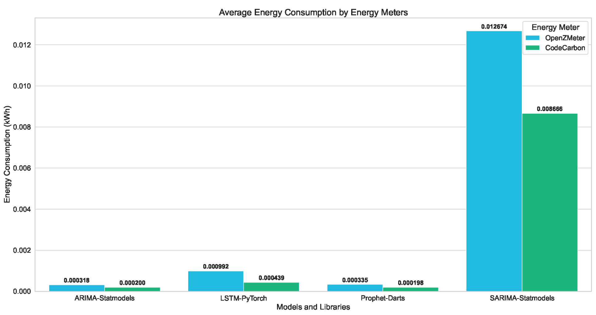
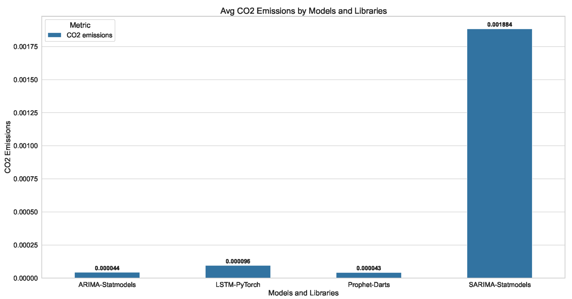
Library	Avg Energy (kWh)		${\mathrm{CO}}_2$ Emissions (kgs)	MAE	RMSE
	oZm	CC
ARIMA
Darts	0.000336	0.000233	0.000051	0.164000	0.188000
Statmodels	0.000318	0.000200	0.000044	0.105000	0.122000
LSTM
Darts	0.002428	0.000967	0.000210	0.136533	0.168400
Keras	0.001591	0.000705	0.000153	0.149600	0.173667
PyTorch	0.000992	0.000439	0.000096	0.133533	0.154067
TensorFlow	0.002061	0.000877	0.000191	0.144000	0.167000
Prophet
Darts	0.000335	0.000198	0.000043	0.070000	0.083000
Prophet	0.001157	0.000705	0.000153	0.099000	0.117000
SARIMA
Statmodels	0.012674	0.008666	0.001884	0.050000	0.063000

Note: The bold rows correspond to the best-performing libraries of each model based on RMSE and MAE.

.

Figure 1 illustrates the average energy consumption in kilowatt–hours (kWh) for different models and libraries, as measured by two energy meters: openZmeter and CodeCarbon. The models evaluated include ARIMA implemented with Statsmodels, LSTM using PyTorch, Prophet with Darts, and SARIMA with Statsmodels. The SARIMA model measured by openZmeter shows the highest energy consumption, followed by the same model measured by CodeCarbon. The other models demonstrate a significantly lower energy consumption.

In Figure 2, the root mean square error (RMSE) and mean absolute error (MAE) of different forecasting models implemented with various libraries. The models evaluated include ARIMA with Statmodels, LSTM with PyTorch, Prophet with Darts, and SARIMA with Statmodels. The chart highlights that SARIMA-Statmodels achieves the lowest error rates, indicating superior accuracy, followed by Prophet-Darts, ARIMA-Statmodels, and LSTM-PyTorch.

Figure 3 shows a comparison of average ${\mathrm{CO}}_2$ emissions in kilograms for different machine learning models and libraries. The evaluated models include ARIMA, LSTM, and SARIMA, implemented in libraries such as Darts, Statmodels, Keras, PyTorch, and TensorFlow. The SARIMA model using Statmodels shows the highest emission (0.001884 kgs), while ARIMA with Statmodels and Prophet with Darts exhibit the lowest emissions, with values of 0.000044 kgs and 0.000043 kgs, respectively. These results highlight the importance of considering ${\mathrm{CO}}_2$ emissions when selecting models and libraries, particularly for sustainable development.

4. Discussion

The comparative analysis between different models and libraries reveals several key findings. ARIMA-based models show a significantly lower energy consumption (0.000336 and 0.000318 kWh) than LSTM models (0.002428 kWh). Regarding ${\mathrm{CO}}_2$ emissions, ARIMA is also superior, with average emissions of 0.000051 and 0.000044 kg, versus the higher emissions of LSTM. Additionally, ARIMA implemented with Statmodels demonstrates a better accuracy (MAE of 0.105 and RMSE of 0.122), being more efficient in both energy and accuracy. It is important to note that LSTM is the only model utilizing GPU, while the others use only CPU. LSTM models, although more complex, have a higher resource consumption and longer execution times, which is crucial in real-time applications.

5. Conclusions

This article presents a preliminary analysis indicating that ARIMA models, especially when implemented with libraries such as Statmodels, are significantly more efficient in terms of energy consumption and ${\mathrm{CO}}_2$ emissions, while also providing adequate accuracy. In contrast, although LSTM models offer certain advantages in specific scenarios due to their ability to capture nonlinear relationships and long-term dependencies, their high energy consumption, higher ${\mathrm{CO}}_2$ emissions, and prolonged execution times may limit their applicability in situations where these factors are critical.

Future research could focus on expanding the study to include different types of data and applications to verify whether the current findings hold in other contexts; investigating optimization and compression techniques for LSTM models to reduce their energy consumption and ${\mathrm{CO}}_2$ emissions without sacrificing accuracy; exploring new model architectures that can offer an optimal balance between energy efficiency and accuracy; analyzing the impact of different hardware infrastructures on energy consumption and ${\mathrm{CO}}_2$ emissions to determine optimal configurations; and evaluating the scalability of these models in large-scale systems, considering both the energy aspects and factors of accuracy and execution time.

References

- Kashpruk, N.; Piskor-Ignatowicz, C.; Baranowski, J. Time Series Prediction in Industry 4.0: A Comprehensive Review and Prospects for Future Advancements. Appl. Sci. 2023, 13, 12374. [Google Scholar] [CrossRef]
- Deb, C.; Zhang, F.; Yang, J.; Lee, S.E.; Shah, K.W. A review on time series forecasting techniques for building energy consumption. Renew. Sustain. Energy Rev. 2017, 74, 902–924. [Google Scholar] [CrossRef]
- Chou, J.S.; Tran, D.S. Forecasting energy consumption time series using machine learning techniques based on usage patterns of residential householders. Energy 2018, 165, 709–726. [Google Scholar] [CrossRef]
- Merelo-Guervós, J.J.; García-Valdez, M.; Castillo, P.A. Energy Consumption of Evolutionary Algorithms in JavaScript. In Proceedings of the 17th Italian Workshop, WIVACE 2023, Venice, Italy, 6–8 September 2023; pp. 3–15. [Google Scholar]
- Escobar, J.J.; Rodríguez, F.; Prieto, B.; Kimovski, D.; Ortiz, A.; Damas, M. A distributed and energy-efficient KNN for EEG classification with dynamic money-saving policy in heterogeneous clusters. Computing 2023, 105, 2487–2510. [Google Scholar] [CrossRef]
- Díaz, A.F.; Prieto, B.; Escobar, J.J.; Lampert, T. Vampire: A smart energy meter for synchronous monitoring in a distributed computer system. J. Parallel Distrib. Comput. 2024, 184, 104794. [Google Scholar] [CrossRef]
- Prieto, B.; Escobar, J.J.; Gómez-López, J.C.; Díaz, A.F.; Lampert, T. Energy efficiency of personal computers: A comparative analysis. Sustainability 2022, 14, 12829. [Google Scholar] [CrossRef]
- Weytjens, H.; Lohmann, E.; Kleinsteuber, M. Cash flow prediction: MLP and LSTM compared to ARIMA and Prophet. Electron. Commer. Res. 2021, 21, 371–391. [Google Scholar] [CrossRef]
- Box, G.E.P.; Jenkins, G. Time Series Analysis, Forecasting and Control; Holden-Day, Inc.: Princeton, NJ, USA, 1990. [Google Scholar]
- Schmidt, V.; Goyal, K.; Joshi, A.; Feld, B.; Conell, L.; Laskaris, N.; Blank, D.; Wilson, J.; Friedler, S.; Luccioni, S. CodeCarbon: Estimate and Track Carbon Emissions from Machine Learning Computing. Zenodo 2021. [Google Scholar] [CrossRef]
- Viciana, E.; Alcayde, A.; Montoya, F.G.; Baños, R.; Arrabal-Campos, F.M.; Zapata-Sierra, A.; Manzano-Agugliaro, F. OpenZmeter: An efficient low-cost energy smart meter and power quality analyzer. Sustainability 2018, 10, 4038. [Google Scholar] [CrossRef]
- Seabold, S.; Perktold, J. Statsmodels: Econometric and statistical modeling with python. SciPy 2010, 7, 1. [Google Scholar]
- Abadi, M.; Agarwal, A.; Barham, P.; Brevdo, E.; Chen, Z.; Citro, C.; Corrado, G.S.; Davis, A.; Dean, J.; Devin, M.; et al. TensorFlow: Large-Scale Machine Learning on Heterogeneous Systems. 2015. Available online: https://www.tensorflow.org/static/extras/tensorflow-whitepaper2015.pdf (accessed on 4 July 2024).
- Paszke, A.; Gross, S.; Massa, F.; Lerer, A.; Bradbury, J.; Chanan, G.; Killeen, T.; Lin, Z.; Gimelshein, N.; Antiga, L.; et al. Pytorch: An imperative style, high-performance deep learning library. Adv. Neural Inf. Process. Syst. 2019, 32. [Google Scholar]
- Herzen, J.; Lässig, F.; Piazzetta, S.G.; Neuer, T.; Tafti, L.; Raille, G.; Van Pottelbergh, T.; Pasieka, M.; Skrodzki, A.; Huguenin, N.; et al. Darts: User-friendly modern machine learning for time series. J. Mach. Learn. Res. 2022, 23, 1–6. [Google Scholar]
- Xu, N. Time Series Analysis on Monthly Beer Production in Australia. Highlights Sci. Eng. Technol. 2024, 94, 392–401. [Google Scholar] [CrossRef]
- Han, Z.; Zhao, J.; Leung, H.; Ma, K.F.; Wang, W. A Review of Deep Learning Models for Time Series Prediction. IEEE Sensors J. 2021, 21, 7833–7848. [Google Scholar] [CrossRef]
- Chai, T.; Draxler, R.R. Root mean square error (RMSE) or mean absolute error (MAE)?—Arguments against avoiding RMSE in the literature. Geosci. Model Dev. 2014, 7, 1247–1250. [Google Scholar] [CrossRef]
- Bird, J. Electrical and Electronic Principles and Technology; Routledge: London, UK, 2017. [Google Scholar]
- Bouza, L.; Bugeau, A.; Lannelongue, L. How to estimate carbon footprint when training deep learning models? A guide and review. Environ. Res. Commun. 2023, 5, 115014. [Google Scholar] [CrossRef] [PubMed]
- Akiba, T.; Sano, S.; Yanase, T.; Ohta, T.; Koyama, M. Optuna: A Next-Generation Hyperparameter Optimization Framework. In Proceedings of the 25th ACM SIGKDD International Conference on Knowledge Discovery & Data Mining, Anchorage, AK, USA, 4–8 August 2019; pp. 2623–2631. [Google Scholar]