Abstract
One of the key challenges for (fresh produce) retailers is achieving optimal demand forecasting, as it plays a crucial role in operational decision-making and dampens the Bullwhip Effect. Improved forecasts holds the potential to achieve a balance between minimizing waste and avoiding shortages. Different retailers have partial views on the same products, which—when combined—can improve the forecasting of individual retailers’ inventory demand. However, retailers are hesitant to share all their individual data. Therefore, we propose an end-to-end graph-based time series forecasting pipeline using a federated data ecosystem to predict inventory demand for supply chain retailers. Graph deep learning forecasting has the ability to comprehend intricate relationships, and it seamlessly tunes into the diverse, multi-retailer data present in a federated setup. The system aims to create a unified data view without centralization, addressing technical and operational challenges, which are discussed throughout the text. We test this pipeline using real-world data across large and small retailers, and discuss the performance obtained and how it can be further improved.
1. Introduction
One key challenge associated with making operational decisions in a logistics and sales context is the accurate forecasting of demand. This is especially true for fresh food retailers. A heightened precision in demand forecasting holds the potential to achieve a balance between minimizing waste (arising from excessive orders of perishable items) and avoiding shortages (caused by insufficient stock for consumers).
To understand the main phenomenon behind the inefficiencies in a retail supply chain, we first detail the Bullwhip Effect (BWE), which refers to the increasing inventory swings in response to changes in consumer demand. Small changes in demand at the retail level can become amplified when moving up the supply chain as shown by the red curve in Figure 1. While first described in 1961 by Forrester [1], how to minimize the negative impact that a subtle shift in point-of-sale demand can cause on the efficiency of the whole supply chain is still being investigated. For retailers, the BWE reflects the inability to cope with unexpected events and food waste, imposing extra challenges when focusing on fresh but highly perishable food. Figure 1 illustrates the amplification generated by BWE and how the supply chain can benefit from quality improvement in purchasing decisions. Note that this is a multi-stakeholder problem [2,3]. Tackling the BWE and creating economic and environmental impact demand a solution throughout the entire value chain from operational, data, and decision-making perspectives. The foresight of the economic advantages of an end-to-end forecasting pipeline using a federated data ecosystem led to a collaborative Belgian R&D project with large- and small-supply-chain retailers.
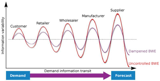
Figure 1.
BWE (red) generates an amplification in the inventory swings alongside the supply chain in response to changes in consumer demand. The purple curve shows how data sharing and enhanced forecasting damps BWE in the whole chain (SOURCE: imec ICON project AI4Foodlogistics proposal).
Firstly, improving forecast accuracy is a must, since less-than-optimal decisions made by supply chain stakeholders at any point along the chain can greatly affect waste, e.g., when too many units of a perishable product are ordered, or can produce shortages, e.g., when products cannot be delivered in time in case of delivery problems or when there is a demand prediction error, which ultimately affects the company’s costs and profitability.
Besides the accuracy of the forecast, our solution must consider other points necessary for adoption by the industry, which is not eager to share data since sales information has important strategic value, influencing when, how, and what information can be accessed and by who. Hence, innovations on the use of downstream demand data and the external integration of non-proprietary data are needed as the precision of a forecasting algorithm highly depends on which data are available, and specifically on the variety of data: different retailers within the supply chain have partial views on the same products, and combining data from different retailers can result in better forecasting of each individual retailer’s inventory demands. In addition, our solution must align with real-time requirements, mainly determined by the moment that information is available and when the forecasts must be used, thus creating a compromise between the accuracy of the proposed model and its time complexity.
The solution we present here is an end-to-end federated forecasting ecosystem pipeline. In essence, the deep learning model providing the forecasting is a generalization of classical recurrent neural networks and convolutional networks for data depicted by an arbitrary graph. The structured sequences, which are used throughout the pipeline, represent the time series of sales and other covariates. The model captures both temporal dependency and structure dynamics. We illustrate with this end-to-end pipeline that the combination of graph deep learning and federated learning capitalizes on their respective strengths to create a potent analytical framework. Graph deep learning’s ability to comprehend intricate relationships harmonizes seamlessly with the diverse, multi-retailer data present in a federated setup. This synthesis results in more robust, accurate, and adaptable forecasting models, ultimately driving better decision-making for all retailers involved.
The main contributions in this paper are (a) the assembly of a federated pipeline, tested in real-time production, that provides a uniform data view from the different retailers without centralizing the data and produces demand forecasts; (b) a discussion of the technical challenges in assembling this pipeline; and (c) the performance evaluation of this pipeline vis-à-vis operational restrictions.
The remainder of this paper is structured as follows: We start with a description of the end-to-end pipeline (Section 2), followed by an explanation of the deep learning model used by the pipeline (Section 3). Since the operation of the pipeline is time-constrained, we discuss its performance in Section 4. Finally, our conclusions are drawn in Section 5.
2. Pipeline Design
Typically, ETL (Extract, Transform, and Load) pipelines are targeted towards single data providers. Therefore (competitive) retailers are not eager to share all their data in a (centralized) data warehouse to train, among others, forecasting algorithms. To tackle this, we propose an end-to-end inventory demand forecasting pipeline using a federated data ecosystem (FDE), illustrated in Figure 2, which provides a uniform data view from the different retailers without centralizing all data or all data structures, and feeds a retailer-independent forecasting model. This generic and extensible setup allows more heterogeneous data to be taken into account when forecasting inventory demand or when executing other data analysis tasks, whilst keeping the retailers in control of which data to share. Traditional approaches expect that all data are integrated in a centralized way. A federated data architecture, allowing queries over decentralized Knowledge Graphs (KGs), avoids the need to centralize data from different retailers, breaking the barriers between stakeholders’ data and decision-making.
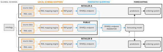
Figure 2.
RML rules describe how source data are mapped to RDF graphs using a common ontology. RML mapping engines execute the rules. SPARQL endpoints expose the RDF graphs. An additional SPARQL Endpoint (Federator) combines the exposed RDF graphs to feed the forecasting model that generates order predictions. Retailers stay in control of their own data, whilst contributing to a retailer-independent forecasting model.
Our FDE consists of three high-level components (global schema, local schema mapping, federated querying) used by the forecasting model. We maximally rely on existing Semantic Web standards to keep the system generic and interoperable.
In the global schema, data are handled via the Resource Description Framework (RDF) [4], organizing data as a graph including semantic context and meaningful relationships between entities. This graph structure allows features to be gradually added to the data model during development or production. All RDF resources are globally identifiable using Uniform Resource Identifiers (URIs), and the schema is modeled as a machine-interpretable ontology using RDF Schema (RFDS) [5]. Combining RDF and RDFS provides global identifiers using a common data model shared and accessed across retailers, allowing for reuse in other use cases.
Local schema mapping is needed to map the source data onto the global schema. These source data consist of both individual retailer data and public data (retrieved from the web using purpose-built programs), and are located in multiple heterogeneous sources and formats (e.g., SQL databases, CSV files, and JSON files). We employ the RDF Mapping Language (RML) [6], a language to define declarative rules to transform heterogeneous source data to a global schema in RDF using a common ontology, independent from the implementation that executes them. Retailers can control which data are shared by only defining those rules that transform the intended data subset in RDF format. The RML rules are executed using RMLStreamer, an MIT-licensed open-source RML mapping engine [7].
Federated querying is achieved via the SPARQL standard to query RDF resources [8]. Each retailer exposes the RDF data produced by the local schema mapping in one SPARQL endpoint, i.e., an access point on an HTTP network that is capable of receiving and processing SPARQL queries. The access to the SPARQL endpoints can be secured by existing authentication methods used in a web context. The FDE is extended with a SPARQL endpoint that exposes publicly available data, e.g, weather conditions, holidays, COVID-19 deaths. An additional SPARQL endpoint acts as federator, i.e., it executes the federated queries over the individual retailer’s endpoints; sub-queries are sent to individual endpoints, and the sub-results are combined to create the complete result. RDF’s graph structure and global identification technique allows for seamless and flexible integration of disparate sources. All SPARQL endpoints were set up using Apache Jena Fuseki [9].
The forecasting model, which we discuss in Section 3, uses the structure of the global schema to formulate queries against the SPARQL endpoint, remaining independent of the individual retailer’s data sources.
In this end-to-end pipeline, retailers stay in control of their own data, whilst contributing to a retailer-independent forecasting model, as the local schema mapping and exposure of the RDF graph can be performed on the retailer’s infrastructure. The FDE allows various sources to register independently of each other (increasing loose coupling and flexibility) and enable detailed descriptions of the original data source. On top of that, by using global identifiers in RDF we can align identifiers across retailers and data sources without performing expensive join operations [10].
3. Forecasting Model
Traditional forecasting methods (a.k.a., state-of-practice models) like ARIMA and VAR focus on relationships between variables and past observations, while traditional deep learning models struggle with spatial relationships in time series data, limiting their efficiency in processing space–time dependencies. To address this limitation, our model as proposed in [11] and shown in Figure 3 uses a graph-based approach using graph neural networks (GNNs) that performs spatio-temporal regressive forecasting with attention, which captures the spatio-temporal relationships that traditional methods overlook. Non-linear and machine learning (ML) methods use data-driven rather than statistical models. State-of-the-art studies show that the increased generality of those models provides more accurate forecasts, especially for volatile products where patterns are difficult to find and traditional statistics fail [12].
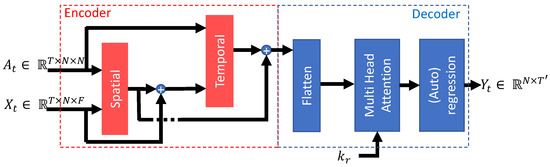
Figure 3.
Proposed spatio-temporal graph-based deep learning model.
This approach allows various external influences to be easily incorporated, e.g., promotions, weather condition, holidays, and interactions with complementary items. Materializing causal relationships between the demand in products and categories and mapping the influence of a change in demand or price on other categories improve product demand forecasting. The products are represented by graph nodes, and edges are created if two products have some kind of relation, e.g., co-purchase, substitution, or joint promotion. This approach characterizes complex relationships between different objects of interest, such as sales in different restaurants, using nodes and edges in a graph representation as shown in Figure 4. In this type of representation, nodes, edges, and the graph itself may have associated properties, which vary (or not) over time. As indicated in the figure, even the connection between nodes can vary over time. The model’s task can be classifying nodes or the graph as a whole, or predicting nodes’/edges’, characteristics or predicting links between nodes. Our model forecasts the features of the nodes using a temporal series of graphs.
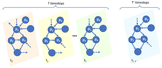
Figure 4.
A time-evolving graph in which four nodes correspond to four products. Given the observations and graph snapshots in the past M time steps, where for each step each node has some feature values, we want to infer in the next time steps the values for these features. The graph can be directed (as above) or undirected (no arrows).
The proposed model consists of a set of layers as shown in Figure 3. The architecture can be seen as an encoder-decoder, where the first two layers encode the data, and the rest corresponds to the decoder. The model takes two required inputs and one optional input. Given N the number of nodes in the graph and T the length of the input data, i.e., the number of days/weeks/months used to train the prediction model, the mandatory inputs are , which represent the series of the adjacency matrix of the graph up to time t, i.e., the series of edge configurations as shown in Figure 4, and , a matrix with the time series of the F variables assigned to the graph nodes used in the forecast, i.e., the series of values of the node characteristics used to feed the model. The first layer processes the spatial information (the relationships between the nodes). The second layer processes temporal information, i.e., how values evolve in time. These layers use self-attention, i.e., the input is used as the attention key to select the relevant information. A residual connection transmits to the temporal layer the original information in the graph, i.e., the original matrix, which is combined with the first layer’s output—acting as an information enrichment layer for the temporal layer. The outputs from the first and second layers are combined to create an embedding that contains spatio-temporal information that can be processed by the decoder. An attention layer was added to the proposed model to control how these embeddings will be combined to produce the forecast. There are two options: an explicit key is provided as input for each graph or, if a key is not given, the model assumes self-attention. This external key is crucial when we feed graphs that represent different groups of information. The last layer produces the result , i.e., days of forecasts (length of the output data) for each of the N nodes.
This graph-based model addresses the limitation of traditional time series forecasting by considering the effects of various factors like competition, out-of-stock situations, new product launches, and limited historical data. This approach provides better predictions compared to baseline methods—traditional and deep learning forecasting methods. A more detailed discussion of this model can be seen in our other paper [11] where we discuss the accuracy and flexibility of the model.
4. Performance of the End-to-End Forecasting Pipeline
Some of the limitations of using graph-based spatio-temporal forecasting methods are a longer training time and decrease in data efficiency for thousands of items in hundreds of stores. Since the forecasting pipeline operation is limited by time due to the operational requirements, we evaluate the time required to execute each stage and discuss the expected performance including for future scenarios of an increase in the number of restaurants and products available for sale. The stakeholders also limited the solution to a platform that only uses servers without graphical or tensor processing units. Then, we argue alternative strategies that can be used to further improve current performance.
The remainder of this paper uses a restaurant chain specialized in fresh food as an example. This chain has different types of points of sale. These can be located inside companies, serving only their employees; they can be at street level, open to the entire public; or they can be inside other retailers, serving the people who frequent these places. Each night, the end-to-end pipeline is triggered. Operational data from stakeholders are consolidated and become available around midnight for processing by the pipeline. Predictions are calculated based on the query results. These predictions must be available to store managers at 5 a.m. Thus, the duration of the pipeline processing window is constrained to 5 h. The training data used in the test are from December 2018 to February 2023, and the prototype ran on data from March and April 2023.
4.1. Knowledge Graph Generation
In the first stage of the pipeline, RDF data are generated using the local schema mapping, and loaded into the SPARQL endpoints, using a virtual container instance with three CPUs and 6GiB memory. At the start of the test period, the source data were contained the historical data of the past two years. It took 75 min to generate the RDF data and load them into the SPARQL endpoints (see Table 1).

Table 1.
The data of the FDE were kept up to date using an incremental nightly update process, shown to be considerably faster than a nightly rebuild.
Repeating this every night would consume unnecessary resources and time. Hence, we set up the following three-step process: (i) delete all data from the last seven days in the SPARQL endpoints, (ii) generate the RDF data with source data related to the last seven calendar days, and (iii) upload the generated RDF data into the SPARQL endpoints. The updating process optimized the execution time to 5 min. The overlapping period of six days in the updating process secures the correction of missing or imprecise data in previous runs. The update of data sources is not always timely. Specifically for data sources that are out of our control (e.g., public data sets such as weather data), we deployed fallback procedures, i.e., configuring default values or looking for alternative data sources.
4.2. Knowledge Graph Queries
Data from several different sources must be obtained and appropriately adjusted to the needs of the forecast model. The pipeline must, therefore, assemble a sequence of KGs for each restaurant. Furthermore, as the pipeline steps are distributed, the transmission time of this large volume of data between the two stages must be considered. A virtual machine (VM) was configured for this test to perform the queries. It was a standard Linux machine (Ubuntu server 22.04) with an Intel(R) Xeon(R) CPU E5-2673 v4 @ 2.30 GHz core and 32 GB of RAM (no GPU). Table 2 shows the time needed to download data from the FDE. The prototype evaluates 44 perishable products from three restaurants using 15 days of data. The time per node is around 35 s, which makes querying all nodes very time-consuming if the nodes are requested one-by-one. However, this process can be sped up by requesting all nodes at the same time. Therefore, the queries are processed at the same time, and are downloaded in blocks. Using this approach, the final performance is, at maximum, 205 s per restaurant as we can see on the second line of the table. Even the graph requests can be made in parallel; therefore, this step is kept within the required time constraints. The necessary hardware can be temporarily allocated on a pay-by-use basis. Thus, this burst of demand can be easily met by the service platform used by the stakeholders.
Table 2.
Time needed to download data from the FDE: (a) each node of the graph or (b) the whole graph. Setup: 3 restaurants, input window of 15 days, 44 products.
4.3. Model
In addition to the product quantities, the pipeline handles several features used as covariates. They relate to (a) information external to the restaurants, such as weather information (minimum and maximum temperature and daily precipitation volume), the daily number of COVID-19 cases, and information about public holidays (bank and school); (b) extra information about the product, e.g., if it was on sale and on promotion on a particular day; and (c) information about the point of sale. The product graph is created using co-purchase similarity, i.e., how likely two products are to be sold together. Product pairs are matched for all restaurants weighted by the relative number of occurrences.
Figure 5 shows the total execution time of the forecasting module using several setups. We tested models with several number of restaurants , selling products. Each graph node contains 90 features. The shadow surrounding the lines represent the confidence interval of our measurements. The curves show exponential growth due to the increase in the size of the model’s matrices. The maximum number of restaurants used in the test is larger than the current number of restaurants and within the growth expectation for the next years. For this test, the same VM described in Section 4.2 was used. The graphs were evaluated in sequence and the total time was annotated. The forecasting module executes in less than 1.5 h in the worst case using a single VM. The biggest restriction for executing the forecasting module in the designated VM is the amount of RAM allocated to it, since the model’s matrices become bigger as the number of restaurants, the number of products, and the size of the forecasting window increase. We argue that the model performance can be improved by forecasting each GNN in parallel (e.g., by increasing the number of cores in the VM or having multiple VMs, each handling one graph) or accelerating it with GPU.
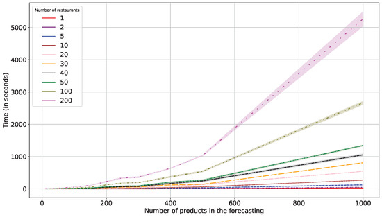
Figure 5.
Forecasting module runtime considering several setups.
Table 3 details the performance of the prototype system, which evaluates 44 perishable products from three restaurants with different target audiences. The evaluation time of the forecast model is at maximum 5 s. The execution time of the module can be divided into three parts: (1) the time to query the graphs from FDE and to download the results from it, (2) the time spent with the model (loading and evaluating), and (3) the time needed to send the forecasts to the server that processes the store’s purchases (upload time). The total time in step (3) is negligible. It only needs to send a low volume of data (a list with 3 + N fields: restaurant code, product code, date, and N forecasted value). According to our measurements, the upload time is ms considering the worst-case scenario—200 restaurants with 1000 products each. Thus, the dominant time is data access, i.e., step (1). Data are requested in parallel by a restaurant/product. However, the forecast is only made when all the data are available. Optimizations can be carried out by (a) performing the prediction as soon as the graph, i.e., all the data from a restaurant, is available, or (b) running multiple models in parallel.
Table 3.
Distribution of runtime: (a) only forecasting or (b) querying and downloading data from FDE, plus computing the model and uploading forecasting to partner’s system. Setup: 3 restaurants, input window of 15 days, 44 products.
4.4. Performance–Accuracy Trade-Off of the Forecasting Model
We showed in [11] that training the model for a single restaurant can generate improvements of up to 86 times in forecast accuracy measured by the root mean square error (RMSE), since restaurants have different customer profiles. However, from a business perspective, there is a trade-off between maintaining multiple forecasting models and accuracy. There is management resistance due to the additional cost in training different versions of the model with hyperparameters adjusted specifically for each case, which may not be compensated by specific savings. Note that RMSE is based only on the error in the number of predicted units. However, this error may occur in products that have little impact on profitability. Using a metric that considers this aspect is beyond the project requirements. Furthermore, multiple models add additional workload for the normally lean technical staff of these companies.
In summary, the prototype forecasting of three restaurants takes less than 12 min to execute all tasks in sequence. For the scenario with 200 restaurants, executing the pipeline stages in sequence is no longer viable, as it would take approximately 13.2 h. However, using the KG request resources in blocks and making the prediction as soon as the data from a restaurant become available, as discussed previously, reduces the total execution time to 04:37:18, keeping the pipeline within the limits defined by the stakeholders. This solution does not use parallelization.
5. Conclusions
The presented inventory demand forecasting pipeline was trialed using real-world data across large and small Belgian retailers. This paper delves into the intricacies of graph-based spatio-temporal forecasting methods, emphasizing their limitations such as extended training times and reduced data efficiency with multiple items. The operational constraints imposed by the stakeholders’ requirements are highlighted. The pipeline operation for the restaurant chain (our practical example) involves nightly triggering of an end-to-end process, consolidating operational data around midnight within a 5 h processing window. KG generation, employing RDF data through local schema mapping and SPARQL endpoints, is discussed, emphasizing the optimization strategy of retaining only the last seven days’ data for nightly runs. The performance results showcase the pipeline evaluation under different setups, The discussion extends to a prototype’s performance, evaluating perishable products from multiple restaurants, with a total evaluation time of less than 12 min, keeping the execution time well below the stipulated limit. Even in the worst-case scenario, execution is kept under 5 h. The breakdown of execution time reveals data access as the predominant factor, prompting a suggestion for optimization and parallelization, and for predicting as soon as all data from a restaurant become available.
The successful trials show that employing RDF/RDFS, SPARQL, and RML allow the application of the same forecasting model independent of the local data source structures. This increases the potentially usable data sources to enrich the model and increase its quality. In future work, we will investigate how to make the pipeline more reactive, e.g., by generating near-real-time data updates from data source to SPARQL endpoint. Along the same line, we will evaluate online model updating strategies (e.g., sampling training), as well as investigate data grouping mechanisms to allow high model accuracy with longer intervals between training. The adoption of a graph-based model adds flexibility regarding the form of the data. The use of a heterogeneous multigraph allows the introduction of different types of relationships between products by incorporating richer semantics into the data. Using a hierarchical model allows different levels of abstraction to be decoupled in the structuring of data; however, this is left for future work.
Author Contributions
All authors participated in the different conceptualization steps, data collection and analysis, interpretation and writing of the manuscript. All authors have read and agreed to the published version of the manuscript.
Funding
The described research activities were supported by the imec ICON project AI4Foodlogistics (Agentschap Innoveren en Ondernemen project nr. HBC.2020.3097).
Institutional Review Board Statement
Not applicable.
Informed Consent Statement
Not applicable.
Data Availability Statement
The data used in the study is private property of the industry partners.
Conflicts of Interest
The authors declare no conflicts of interest.
References
- Forrester, J.W. Industrial dynamics. J. Oper. Res. Soc. 1997, 48, 1037–1041. [Google Scholar] [CrossRef]
- Tsaqiela, B.Q.; Arkeman, Y.; Sanim, B. Reduction of Bullwhip Effect on Commodity Supply Chain in Fresh Fruits and Vegetables Wholesale Lottemart Bogor. Indones. J. Bus. Entrep. (IJBE) 2016, 2, 43. [Google Scholar] [CrossRef][Green Version]
- Rodrigues, V.S.; Demir, E.; Wang, X.; Sarkis, J. Measurement, mitigation and prevention of food waste in supply chains: An online shopping perspective. Ind. Mark. Manag. 2021, 93, 545–562. [Google Scholar] [CrossRef]
- Cyganiak, R.; Wood, D.; Lanthaler, M. RDF 1.1 Concepts and Abstract Syntax. 2014. Available online: https://www.w3.org/TR/rdf11-concepts (accessed on 29 September 2023).
- Brickley, D.; Guha, R.V. RDF Schema 1.1. 2014. Available online: https://www.w3.org/TR/rdf-schema (accessed on 29 September 2023).
- Iglesias-Molina, A.; Van Assche, D.; Arenas-Guerrero, J.; De Meester, B.; Debruyne, C.; Jozashoori, S.; Maria, P.; Michel, F.; Chaves-Fraga, D.; Dimou, A. The RML Ontology: A Community-Driven Modular Redesign after a Decade of Experience in Mapping Heterogeneous Data to RDF. In Proceedings of the International Semantic Web Conference (ISWC), Cham, Switzerland, 6–10 November 2023. Lecture Notes in Computer Science. [Google Scholar]
- Oo, S.M.; Haesendonck, G.; Meester, B.D.; Dimou, A. RMLStreamer. 2022. Available online: https://github.com/RMLio/RMLStreamer (accessed on 29 September 2023).
- Prud’hommeaux, E.; Aranda, C.B. SPARQL 1.1 Federated Query. 2013. Available online: https://www.w3.org/TR/sparql11-federated-query (accessed on 29 September 2023).
- Foundation, A.S. Apache Jena. 2021. Available online: https://jena.apache.org (accessed on 29 September 2023).
- de Vleeschauwer, E.; Min Oo, S.; De Meester, B.; Colpaert, P. Reference Conditions: Relating Mapping Rules Without Joining. In Proceedings of the 4th International Workshop on Knowledge Graph Construction (KGCW 2023) Co-Located with 20th Extended Semantic Web Conference (ESWC 2023), Hersonissos, Greece, 28 May 2023; p. 8. [Google Scholar]
- Moura, H.D.; Kholkine, L.; D’eer, L.; Mets, K.; Schepper, T.D. Towards graph-based forecasting with attention for real-world restaurant sales. In Proceedings of the IEEE International Conference on Data Mining Workshops, Shanghai, China, 4 December 2023. [Google Scholar]
- Tarallo, E.; Akabane, G.K.; Shimabukuro, C.I.; Mello, J.; Amancio, D. Machine learning in predicting demand for fast-moving consumer goods: An exploratory research. IFAC-PapersOnLine 2019, 52, 737–742. [Google Scholar] [CrossRef]


Disclaimer/Publisher’s Note: The statements, opinions and data contained in all publications are solely those of the individual author(s) and contributor(s) and not of MDPI and/or the editor(s). MDPI and/or the editor(s) disclaim responsibility for any injury to people or property resulting from any ideas, methods, instructions or products referred to in the content. |
© 2024 by the authors. Licensee MDPI, Basel, Switzerland. This article is an open access article distributed under the terms and conditions of the Creative Commons Attribution (CC BY) license (https://creativecommons.org/licenses/by/4.0/).