Abstract
This work applies the rarely seen explosive version of autoregressive modelling to a novel practical context—geological failure monitoring. This approach is more general than standard ARMA or ARIMA methods in that it allows the underlying data process to be explosively nonstationary, which is often the case in real-world slope failure processes. We develop and test our methodology on a case study consisting of high-quality (in situ) line-of-sight radar displacement data from a slope that undergoes a failure event. Specifically, we first optimally estimate the characteristic roots of the autoregressive processes underpinning the displacement time series preceding the failure at each monitoring location. We then establish and utilise a pivotal quantity for the autoregressive parameter ensemble to perform simulation-based hypothesis test/s for the explosiveness of the corresponding true characteristic roots. Concluding that a true characteristic root becomes explosive at some significance level implies that the underlying displacement process is explosively nonstationary, and, hence, local geological instability is suspected at this significance level. We found that the actual location of failure (LOF) was identified well in advance of the time of failure (TOF) by flagging those locations where explosive root(s) were identified by our approach. This statistical feedback model for ground motion dynamics presents an alternative and/or addition to the velocity threshold approach to early warning of impending failure.
1. Introduction
Geological failure events, such as landslides, mining accidents, or subsidence, cause massive economic and humanitarian damage globally [1]. With the ultimate aim of mitigating such hazards by providing risk assessment and/or early warning, our statistical modelling approach aims to capture the core dynamical properties of a slope susceptible to failure and presents a novel red alert definition for safety practitioners.
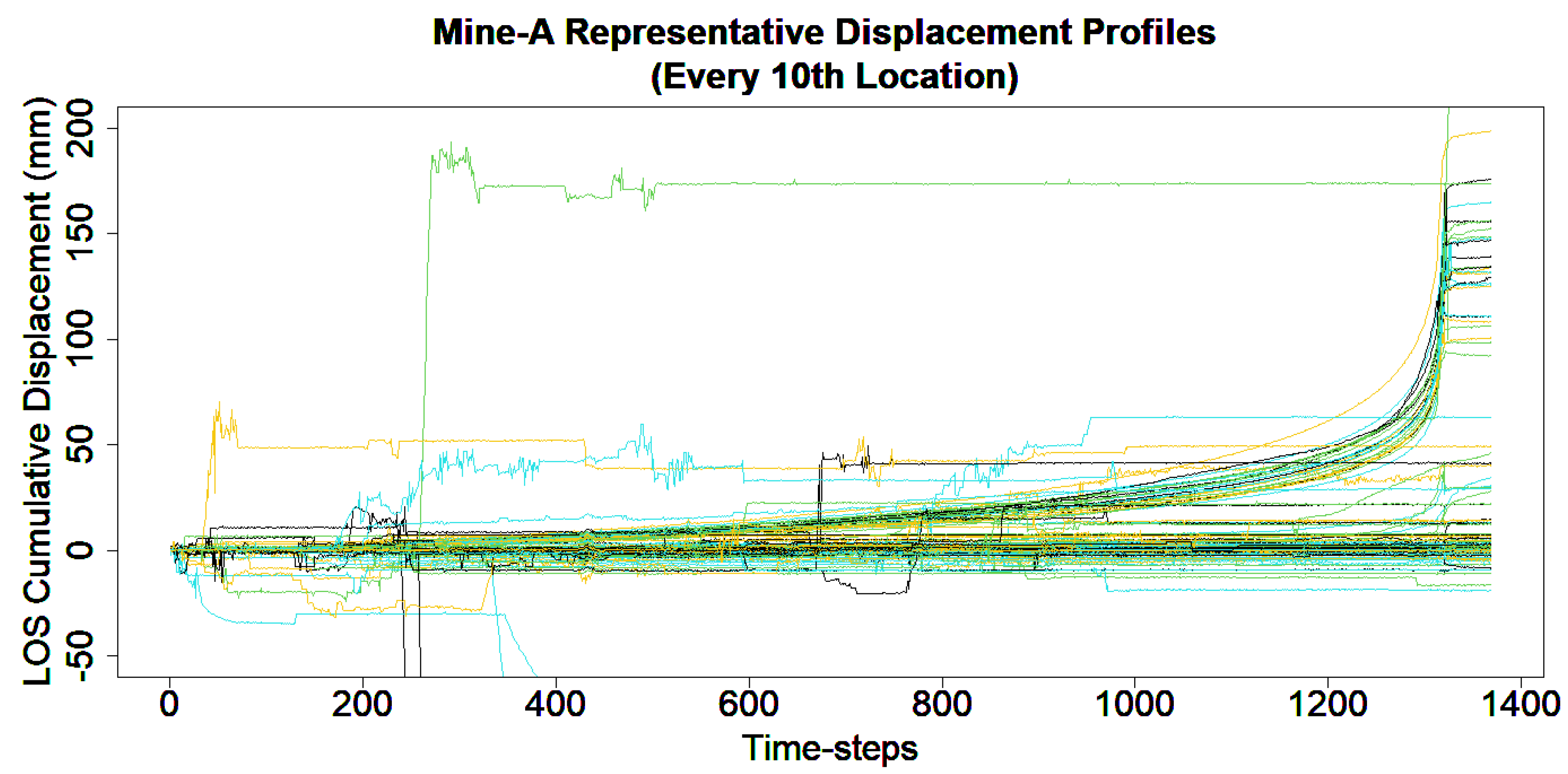
Accurate data are beneficial in making such assessments and we investigate high-quality radar data as a case study. These data have been previously studied in the cutting-edge work contained in [2,3,4], the latter of which proposes a four-pronged approach to risk assessment and automated TOF prediction based on their “EVE” model. EVE uses a logarithmic transformation on the raw displacement values to attempt to deal with the explosive nonstationarity apparent in the data, followed by a cointegration-based approach (with deterministic trend) for the log-displacement values. Our work, in contrast, is only focused on the question of early LOF prediction and does not perform any transformation to deal with explosive nonstationarity, instead modelling this directly with autoregression. Ground motion tracking radar was used to monitor line-of-sight (LOS) ground displacement over a slope and through time, providing spatial lattices of displacement time series. The specific monitored slope comes from an anonymous mining site which we will refer to as “mine-A”. The data consist of ground displacement measurements on 5158 locations (including a subset which suffered a failure event) recorded over 1369 time states of around 6 min each. The 5158 locations constitute a nearly rectangular spatial grid with a resolution of around 7 by 7 m. The time of failure was identified as time step 1315. Figure 1 presents the cumulative displacement profiles of every 10th location (to reduce clutter). Further details on the technology, LOF, geological details, etc., can be found in the aforementioned references.

Figure 1.
Mine-A representative cumulative displacement profiles (every 10th location). Note that there are several outlying series with drastic changes in displacement and which do not fall within the LOF. Otherwise, two distinct regimes emerge; a relatively stable grouping of time series and a subset which seem to exponentially diverge.
A natural statistical framework to capture the temporal dependence among such data are autoregressive models. However, well-known frameworks such as ARMA or ARIMA [5] assume causal and stationary data (or, at worst, unit root, trend/drift stationary data) [6]. Stationary, causal series representations implicitly place certain restrictions on autoregressive parameters—disallowing unit or explosive roots of the associated “characteristic polynomial”. Stationary time series are also “mean-reverting”. However, displacement time series associated with geological failure events (e.g., landslide) clearly are not mean-reverting, and, thus, are nonstationary phenomena. Hence, classical models make some assumptions that do not agree with the physical laws underpinning the observed data, and this is the essential statistical issue to be addressed in this research.
2. Materials and Methods
We term the AR(p ) process where characteristic roots are not implicitly assumed to be nonexplosive (as they are in traditional presentations of ARMA/ARIMA) “exp-AR(p)”. Concretely, the exp-AR(p) model has the following form:
where s are random variables, in our case representing LOS displacement time series (at a given location). The time index t runs over times, say, , the first p of which are considered known and fixed for conditional least squares purposes. The terms are normal with mean zero and nonzero variance . While are fixed but unknown parameters. Specifically, is commonly termed a “drift” parameter and is of little interest in our setting. The terms are what we call “autoregressive parameters” as they control the stationarity/nonstationarity of the process. Our final assumption (in fact, lack of assumption in contrast to usual AR(p) presentations) is that there are no restrictions on the roots of the characteristic polynomial:
Note that roots of Equation (2) may be complex numbers. If roots of Equation (2) are all inside the unit circle (of the complex plane), then this implies that model (1) is stationary. Having at least one root on the unit circle, with the remainder inside the unit circle, implies random walk nonstationarity, also known as an “unstable” process. If at least one root is outside the unit circle then this implies explosive nonstationarity. Surprisingly, even in the case of explosive nonstationarity, the literature has established consistency and asymptotic pivotal quantities involving the ordinary least squares (OLS) estimators [7] for exp-AR(p) processes. Given our interest in geological failure, we seek to test the null hypothesis of a stationary autoregressive process against an alternative hypothesis of explosive root/s. Note that we do not consider the boundary case of unstable/unit root behaviour. This is equivalent to testing the null hypothesis of all the roots being inside the unit circle against its alternative that some of the roots are outside the unit circle. Our approach is as follows.
Firstly, we estimate the lag order “p” of a given exp-AR(p) process via AIC. Then, the coefficients of model (1) are estimated via conditional least squares (CLS, conditional on the first p values ). This procedure is well known; see, for instance [6]. It yields autoregressive parameter estimates . We denote the vectorised collection of the true/estimated auto-regressive coefficients by and , respectively. We now present the pivotal quantity on which our explosivity analysis is based. In the case, it is known that unless the true root has an absolute value of 1 exactly, then the normalised statistic has limiting standard normal distribution [8]. We verified via simulation study the analogous claim in the case, i.e., that (other than in the presence of a precise unit root) regardless of the explosivity/not of the underlying time series,
where D indicates convergence in distribution or weak convergence, and is the estimated variance–covariance matrix without entries corresponding to the drift term, i.e., the full variance–covariance matrix with the first row and column removed. Since this matrix is positive definite, it has a unique positive definite square root ). This result can also be found (at least in part) in the literature; see [7] (chapter 10.2) or [9] in particular.
Note that, in practice, for small sample sizes, the parameter estimates are known to be biased with skewed probability distributions [10]. Simulation indicates that for the order of sample size used in our context (several hundred at least) and noise levels of the size estimated in our datasets, these effects are negligible. It is also well known that the true covariance matrix is consistently estimated by above and that the parameter estimates of the exp-AR(p) coefficients are consistent [11] (regardless of the explosivity/not of the series).
Using the CLS exp-AR(p) parameter estimates , one can form an estimated version of the characteristic polynomial governing the autoregressive process and solve it to achieve estimates of the characteristic roots. We denote the estimated characteristic polynomial, which simply substitutes in the CLS parameter estimates to Equation (2), by . Finally, we denote the true roots of : and their estimates from : .
With our pivotal quantity at hand, we turn to the topic of hypothesis testing for explosive versus stationary behaviour of a given time series. Since the pivotal quantity is a complicated multivariate expression, it is not immediately obvious how to come up with closed-form expressions relating to the root of largest absolute value. Partial progress can be made utilising multivariate delta methods [12]; however, a much more pragmatic and flexible approach involves simulation. Since the pivotal quantity (asymptotically) applies regardless of the true characteristic root placement, we can test a diversity of hypothesis via simulating a large number of random variables and transforming them with the estimated quantities accordingly.
For instance, consider the null hypothesis of a stationary series versus the alternative of an explosive series (i.e., at least one explosive characteristic root). To test this hypothesis, simply generate some large number (e.g., 10,000) standard-MVN random variables of dimension equal to p. Multiply each of them by and then add (to invert the operations seen in the pivot). Following this, solve for the roots of the characteristic polynomials with coefficients given by the values in each these vectors and look at the proportion of cases where some root has modulus greater than 1. If this is more than 95% of the time, we reject the null hypothesis at a significance level of 5%. One may follow essentially the same approach to test more exotic hypothesis, such as the existence of complex roots (indicative of oscillatory behaviour), explosive or otherwise.
We summarise our procedure for location-wise determination of explosive nonstationarity for mine-A following:
- Take the time series of LOS displacement values at a given location, and call this for .
- Using the CLS estimation method and AIC (for instance) as a model selection criterion, determine the optimal lag order and parameter estimates and of an autoregressive model for of form given in Equation (1).
- Simulate a large ensemble of standard-MVN random variables (e.g., 10,000). Transform each such vector by the inverse operations, as those seen in the pivotal quantity for the true autoregressive parameters given in Equation (3) (multiplication by , then addition of ).
- Use numerical methods to estimate the roots of the characteristic polynomial associated with each such simulated vector.
- Accept/reject the null hypothesis based on the proportion of simulation cases where one or more of the p roots found is explosive. For instance, if 95% or more of simulations indicate explosive behaviour, reject the null to have a 5% significance level.
3. Results and Discussion
Our methodology was applied location-wise to mine-A over varying levels of training set size. To be precise, training sets comprised subsets of the full time series consisting of only the first few consecutive times, e.g., times 1–300 or 1–1000. This was to assess at what stage before failure it was possible to confidently flag explosive nonstationarity, and, hence, risk of failure. For completeness, we also present results pertaining to the (largest in modulus) root estimates themselves. We worked within the R computing environment to perform our analysis [13].
We found that a clear region mirroring the eventual LOF was identified as having explosive root estimates after only the first 200 time increments were allowed in training. More precisely, Figure 2 shows maps of the locations coloured according to the (largest in modulus) roots estimated there. The eventual LOF is already clearly represented here and this pattern persists for training windows of increasing size (e.g., 1000 or 1310 just before failure). Note that due to the smooth colour ramp used, it may seem as though many locations outside of the LOF could be explosive; however, this is actually very rarely the case. That is to say, points outside the LOF may have characteristic roots quite close to 1; however, they are almost always only nearly nonstationary.
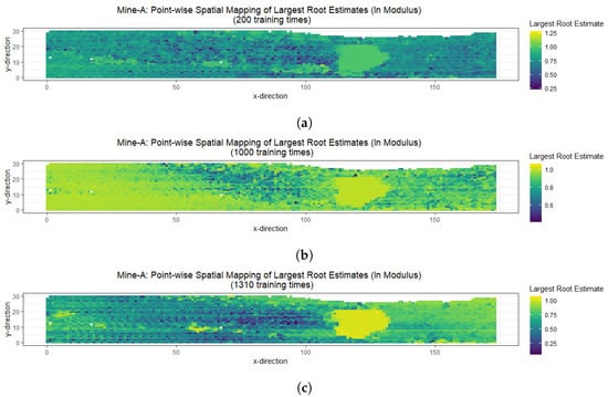
Figure 2.
Spatial maps of estimated roots over Mine-A locations. (a) Map of Mine-A locations, coloured according to the value of the largest modulus of the characteristic roots estimated at each location. The first 200 training times were used from the total 1315 prefailure times. A clear ovular region of points identified as near-explosive already emerges in the centre-right. (b) Map of Mine-A locations, coloured according to the value of the largest modulus of the characteristic roots estimated at each location. The first 1000 training times were used from the total 1315 prefailure times. Note that it may appear (due to the gradual nature of colouration) to some viewers that a large portion of the slope is now explosive; however, the surrounding regions are typically slightly below a value of one and, hence, are still stationary. In fact, more or less, only those points in the eventual LOF actually sometimes exceed a value of 1. (c) Map of Mine-A locations, coloured according to the value of the largest modulus of the characteristic roots estimated at each location. The first 1310 training times were used from the total 1315 prefailure times. The ovular region of points identified as explosive is now quite stark.
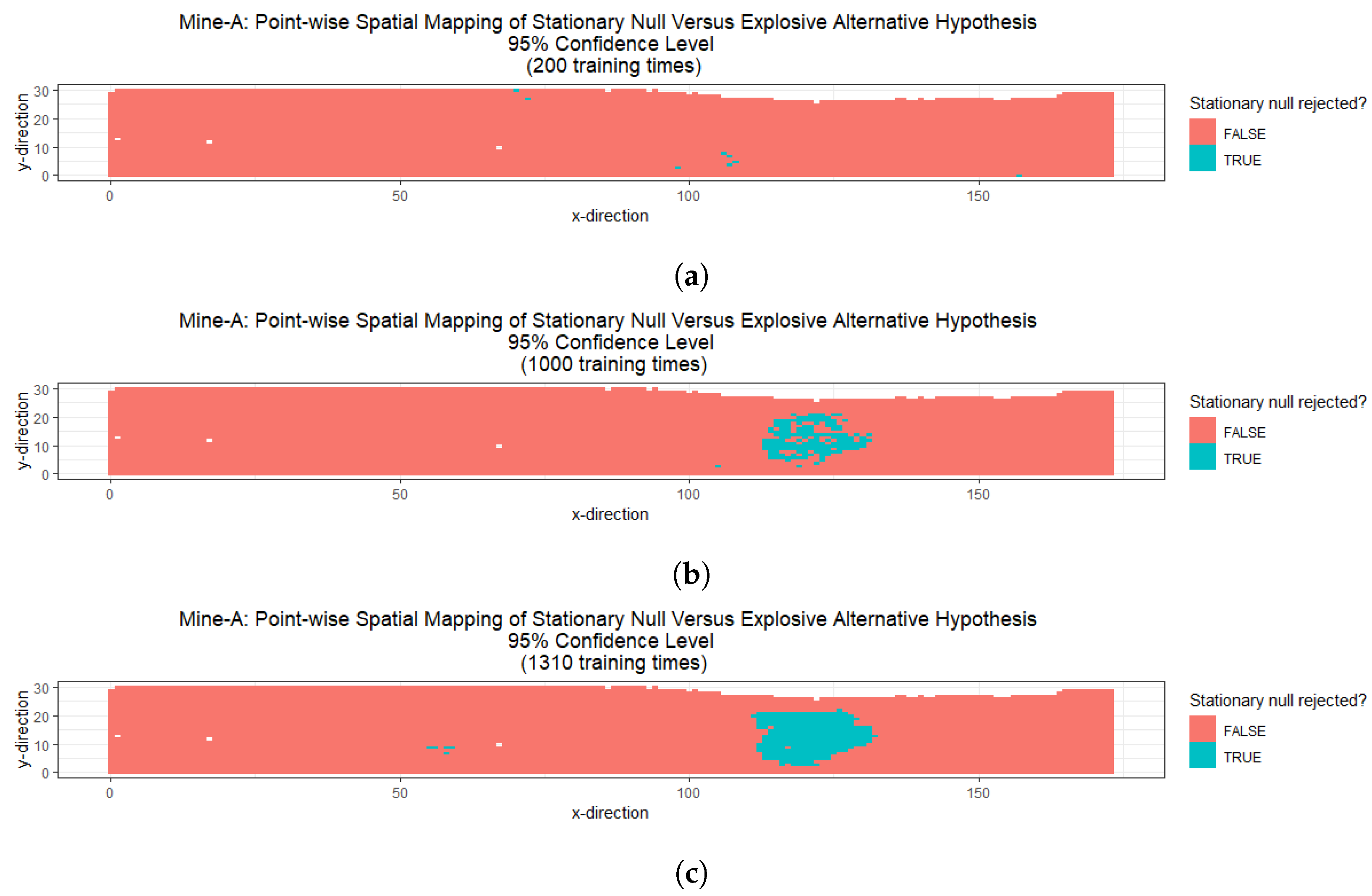
However, regarding our testing procedure, with a null hypothesis of stationarity and what might be viewed as a very skeptical confidence threshold of 95%, it takes more training data until the null is confidently rejected over the eventual failure region. By comparison, after 200 training times, essentially no locations are flagged as explosive at the stringent 95% confidence threshold (refer to Figure 3). With 1000 training times used, the eventual LOF is predicted quite well by the emerging region of flagged locations. Right before failure (1310 training times), the failure zone (independently known from [2,3]) is essentially perfectly recreated.
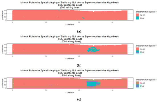
Figure 3.
Spatial maps of stationary versus explosive hypothesis test outcomes over Mine-A locations. (a) Map of Mine-A locations, coloured according to whether our simulation-based hypothesis testing scheme accepts/rejects the null hypothesis of stationarity at a confidence level of 95% (location-wise). The first 200 training times were used from the total 1315 prefailure times. The previously seen ovular region of points identified as explosive is yet to emerge at this high threshold of confidence (however, it does so clearly at lower thresholds of confidence). (b) Map of Mine-A locations, coloured according to whether our simulation-based hypothesis testing scheme accepts/rejects the null hypothesis of stationarity at a confidence level of 95% (location-wise). The first 1000 training times were used from the total 1315 prefailure times. The eventual LOF is clearly emerging. (c) Map of Mine-A locations, coloured according to whether our simulation-based hypothesis testing scheme accepts/rejects the null hypothesis of stationarity at a confidence level of 95% (location-wise). The first 1310 training times were used from the total 1315 prefailure times. The ovular region of points identified as explosive is now clearly identified.
If one reverses their perspective regarding the null/alternative of the hypothesis test, then the failure region is flagged much earlier (again after around 200 time steps), i.e., if the null hypothesis is that each given series is explosive, then the failure region is more quickly identified, as one may expect. It is of course up to the practitioner which perspective they might take. For instance, if monitoring a slope at random, one might assume its constituents are stationary until proven otherwise, while if a slope is suspected to be unstable due to some forewarning signs (e.g., cracking observed), it would be reasonable to take the opposite perspective in the interest of safety.
We also point out that our hypothesis testing regime is on a point-by-point basis. We are encouraged by the fact that when looking at the ensemble of points where we accept/reject the null, this seems to reflect the eventual LOF. However, strictly speaking, we have not given an aggregate test that some given region is at risk. For this, simple multiple testing measures could be used. Alternatively, hypothesis testing ideas from spatial statistics literature may be helpful to practitioners interested in testing whether a certain region as a whole is at risk.
In conclusion, we show, using only LOS displacement data derived from radar sources, that markedly early indication of the LOF is possible for a real-world example of geological failure. Furthermore, a novel criterion for early warning is given, namely, the identification (to desired level of confidence) of explosive nonstationarity. This requires no extraneous domain knowledge of specific geological properties (á la empirical velocity thresholds). The method is based on estimation of the explosivity of the autoregressive parameter ensemble perceived to govern each point’s displacement time series. This is all made possible by the utilisation of a key pivotal quantity given in Equation (3), which maintains its distribution regardless of the stationarity/otherwise of the underlying time series. Computational resources required for these assessments are minimal and could be carried out in real time. In fact, all analysis for this paper was carried out on a basic laptop with an i5 processor and 8 GB of RAM. The statistical concepts are also accessible to practitioners as they are largely based on linear regression, autoregression, and simulation. It remains a topic of interest how this finding extends to other kinds of failure events, geologies/materials, and geometries.
Author Contributions
Conceptualization, M.M. and G.Q.; methodology, M.M. and G.Q.; simulation, M.M.; writing—original draft preparation, M.M.; writing—review and editing, M.M., G.Q. and A.T.; data curation and acquisition, A.T. All authors have read and agreed to the published version of the manuscript.
Funding
This research was completed as part of the Ph.D. studies of M.M., funded by a Research Training Program Scholarship (Stipend). This was provided by the Australian Government Research Training Program and the University of Melbourne.
Institutional Review Board Statement
Not applicable.
Informed Consent Statement
Not applicable.
Data Availability Statement
Data sharing is not applicable due to privacy.
Acknowledgments
The authors are mainly thankful to the University of Melbourne (Unimelb), who provided the opportunity to conduct this research.
Conflicts of Interest
The authors declare no conflicts of interest.
References
- Sim, K.; Lee, M.; Wong, S. A review of landslide acceptable risk and tolerable risk. Geoenviron. Disasters 2022, 9, 3. [Google Scholar]
- Tordesillas, A.; Kahagalage, S.; Campbell, L.; Bellett, P.; Batterham, R. Introducing a data-driven framework for spatiotemporal slope stability analytics for failure estimation. In SSIM 2021: Second International Slope Stability in Mining; Australian Centre for Geomechanics: Perth, Australia, 2021; pp. 235–246. Available online: https://papers.acg.uwa.edu.au/p/2135_14_Tordesillas/ (accessed on 24 March 2024).
- Tordesillas, A.; Kahagalage, S.; Campbell, L.; Bellett, P.; Intrieri, E.; Batterham, R. Spatiotemporal slope stability analytics for failure estimation (SSSAFE): Linking radar data to the fundamental dynamics of granular failure. Sci. Rep. 2021, 11, 9729. [Google Scholar] [CrossRef] [PubMed]
- Tordesillas, A.; Zheng, H.; Qian, G.; Bellett, P.; Saunders, P. Augmented Intelligence Forecasting and What-If-Scenario Analytics with Quantified Uncertainty for Big Real-Time Slope Monitoring Data. IEEE Trans. Geosci. Remote. Sens. 2024, 62, 1–29. [Google Scholar] [CrossRef]
- Pfaff, B. Analysis of Integrated and Cointegrated Time Series with R; Springer: New York, NY, USA, 2008. [Google Scholar]
- Shumway, R.; Stoffer, D. Time Series Analysis and Its Applications, with R Examples, 4th ed.; Springer: Cham, Switzerland, 2017. [Google Scholar]
- Fuller, W. Introduction to Statistical Time Series, 2nd ed.; Wiley: New York, NY, USA, 1996. [Google Scholar]
- Anderson, T. On Asymptotic Distributions of Estimates of Parameters of Stochastic Difference Equations. Ann. Math. Stat. 1959, 30, 676–687. Available online: https://api.semanticscholar.org/CorpusID:121146661 (accessed on 2 March 2024). [CrossRef]
- Monsour, M.; Mikulski, P. On limiting distributions in explosive autoregressive processes. Stat. Probab. Lett. 1998, 37, 141–147. Available online: https://www.sciencedirect.com/science/article/pii/S0167715297001119 (accessed on 8 March 2024). [CrossRef]
- Shaman, P.; Stine, R. The Bias of Autoregressive Coefficient Estimators. J. Am. Stat. Assoc. 1988, 83, 842–848. Available online: http://www.jstor.org/stable/2289315 (accessed on 18 March 2024). [CrossRef]
- White, J. The Limiting distribution of the serial correlation coefficient in the explosive case. Ann. Math. Stat. 1958, 29, 1188–1197. Available online: https://api.semanticscholar.org/CorpusID:122153366 (accessed on 6 March 2024). [CrossRef]
- Hoef, J. Who Invented the Delta Method? Am. Stat. 2012, 66, 124–127. Available online: http://www.jstor.org/stable/23339471 (accessed on 6 March 2024). [CrossRef]
- R Core Team. R: A Language and Environment for Statistical Computing; R Foundation for Statistical Computing: Vienna, Austria, 2013; Available online: http://www.R-project.org/ (accessed on 2 March 2024).
Disclaimer/Publisher’s Note: The statements, opinions and data contained in all publications are solely those of the individual author(s) and contributor(s) and not of MDPI and/or the editor(s). MDPI and/or the editor(s) disclaim responsibility for any injury to people or property resulting from any ideas, methods, instructions or products referred to in the content. |
© 2024 by the authors. Licensee MDPI, Basel, Switzerland. This article is an open access article distributed under the terms and conditions of the Creative Commons Attribution (CC BY) license (https://creativecommons.org/licenses/by/4.0/).