Proceeding Paper

JET: Fast Estimation of Hierarchical Time Series Clustering †

1
Hasso Plattner Institute, University of Potsdam, 14469 Potsdam, Germany
2
Rolls-Royce Deutschland Ltd. & Co. KG, 15827 Blankenfelde-Mahlow, Germany
3
Department of Mathematics and Computer Science, Philipps University of Marburg, 35037 Marburg, Germany
*
Author to whom correspondence should be addressed.
Presented at the 10th International Conference on Time Series and Forecasting, Gran Canaria, Spain, 15–17 July 2024.
Eng. Proc. 2024, 68(1), 37; https://doi.org/10.3390/engproc2024068037
Published: 11 July 2024
(This article belongs to the Proceedings of The 10th International Conference on Time Series and Forecasting)

Abstract

:
Clustering is an effective, unsupervised classification approach for time series analysis applications that suffer a natural lack of training data. One such application is the development of jet engines, which involves numerous test runs and failure detection processes. While effective data mining algorithms exist for the detection of anomalous and structurally conspicuous test recordings, these algorithms do not perform any semantic labeling. So, data analysts spend many hours connecting the large amounts of automatically extracted observations to their underlying root causes. The complexity, number, and variety of extracted time series make this task hard not only for humans, but also for existing time series clustering algorithms. These algorithms either require training data for supervised learning, cannot deal with varying time series lengths, or suffer from exceptionally long runtimes. In this paper, we propose JET, an unsupervised, highly efficient clustering algorithm for large numbers of variable-lengths time series. The main idea is to transform the input time series into a metric space, then apply a very fast conventional clustering algorithm to obtain effective but rather coarse-grained pre-clustering of the data; this pre-clustering serves to subsequently estimate the more accurate but also more costly shape-based distances of the time series and, thus, enables JET to apply a highly effective hierarchical clustering algorithm to the entire input time series collection. Our experiments demonstrate that JET is highly accurate and much faster than its competitors.

1. Introduction

Time Series Anomaly Detection (TSAD) is the task of finding subsequences in a time series that are maximally different from the rest of the time series. Because anomalies often indicate special events, such as heart failures in cardiology [1], structural defects in jet turbine engineering [2], or ecosystem disturbances in earth sciences [3], numerous TSAD algorithms with different detection approaches have been published in the past few years [4,5,6,7]. These algorithms range from deep learning approaches [8,9] over data mining techniques [10,11] to classical statistical methods [12,13]. Most of these algorithms are either semi-supervised or unsupervised and, thus, do not learn the shape of anomalies from training data. Instead, they find anomalous subsequences by comparing them either to other patterns in the time series or to an internal (learned) model of normal behavior [7]. For this reason, TSAD algorithms can discover interesting subsequences, but they cannot classify what they have found: Their output is (usually) a one-dimensional anomaly score that indicates only the degree of abnormality at a certain timestamp, but it does not distinguish or classify anomalous behavior. For this reason, anomaly detection processes are usually accompanied by classification steps that differentiate between different types of anomalies, such as Marked Crisis vs. Black Friday, Engine Misfire vs. Bird Impact, or Known Error vs. Unknown Error. If no training data are available for the classification, which is usually the case for unsupervised and semi-supervised anomaly detection runs, classification is performed via (time series) clustering. Via clustering, scientists can connect certain anomalies with their respective motives and find groups of automatically detected anomalies with shape-wise and, hence, hopefully, also semantically similar types.
Because anomalous time series subsequences often vary in length, many standard clustering algorithms cannot handle them appropriately. Furthermore, TSAD jobs often target Terrabytes of time series data in smart sensing applications, industrial engineering, logistics systems, and many further applications; they therefore often produce Gigabytes of anomalous time series, which, when processed with state-of-the-art clustering algorithms, result in performance issues.
To tackle the quality and performance issue, we propose the novel time series clustering algorithm JET. JET, which is an acronym for Jaunty Estimation of Hierarchical Time Series Clustering, is an approximated version of shape-based hierarchical clustering (HC). In a preprocessing step, the algorithm uses a fast but only coarse-grained clustering approach on an embedded representation of the input time series to find a relatively high number of clusters. The distances between the centers of these clusters are then used to estimate the distances between the time series of different clusters. Thereof, an estimated distance matrix can be generated that serves as an input parameter for an exhaustive HC algorithm. More specifically, our paper makes the following contributions:
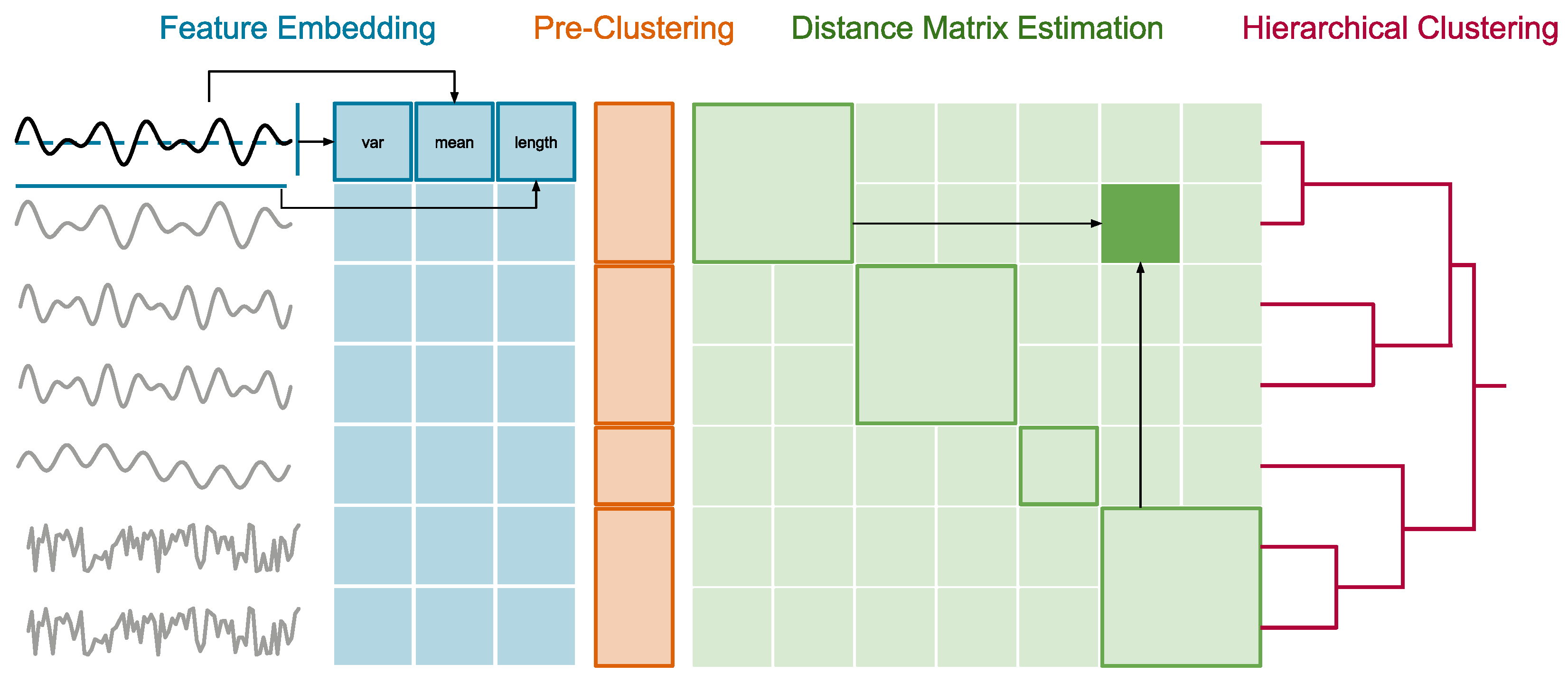
  • Time Series Clustering via JET: We propose the approximate HC algorithm JET, which (1) embeds arbitrary long time series into a fixed-sized space by extracting representative time series features, (2) runs fast but coarse-grained pre-clustering with a pessimistically high number of groups, (3) approximates group-to-group time series distances with the centroid distances of the groups, and (4) calculates full hierarchical clustering with the partially approximated, but still highly accurate, distances (Section 4).
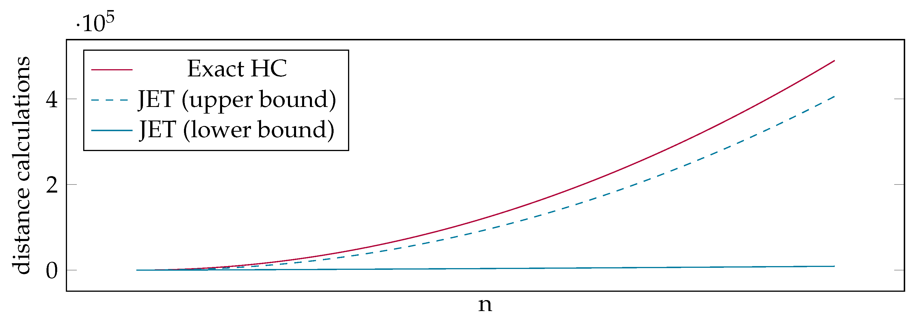
  • Theoretical Runtime Analysis of JET: We provide a theoretical analysis of our distance matrix estimation by calculating the best and worst case runtimes. Our analysis shows that even in the worst case, JET is significantly faster than an exact calculation of the entire distance matrix (Section 5).
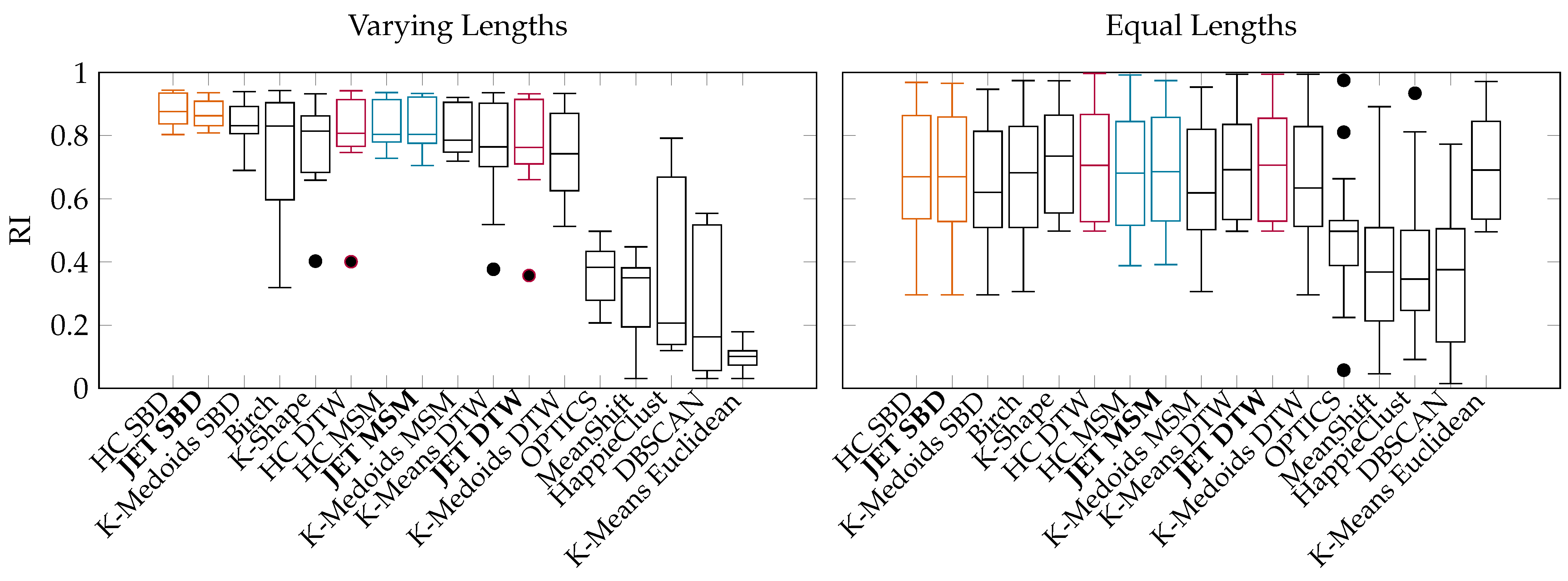
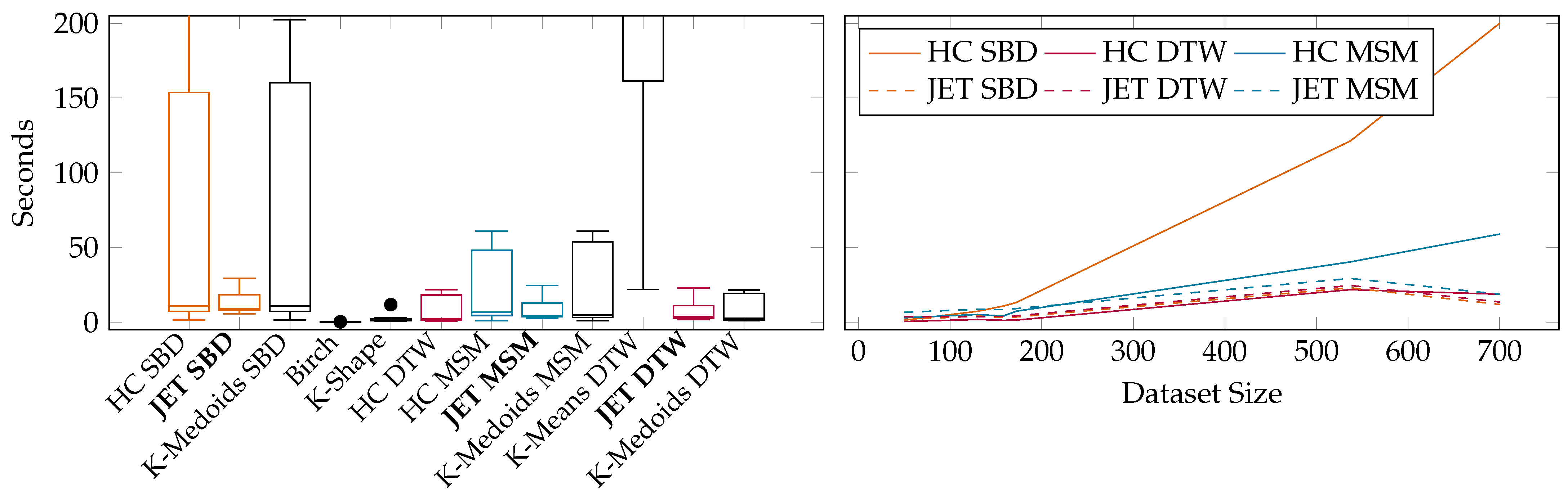
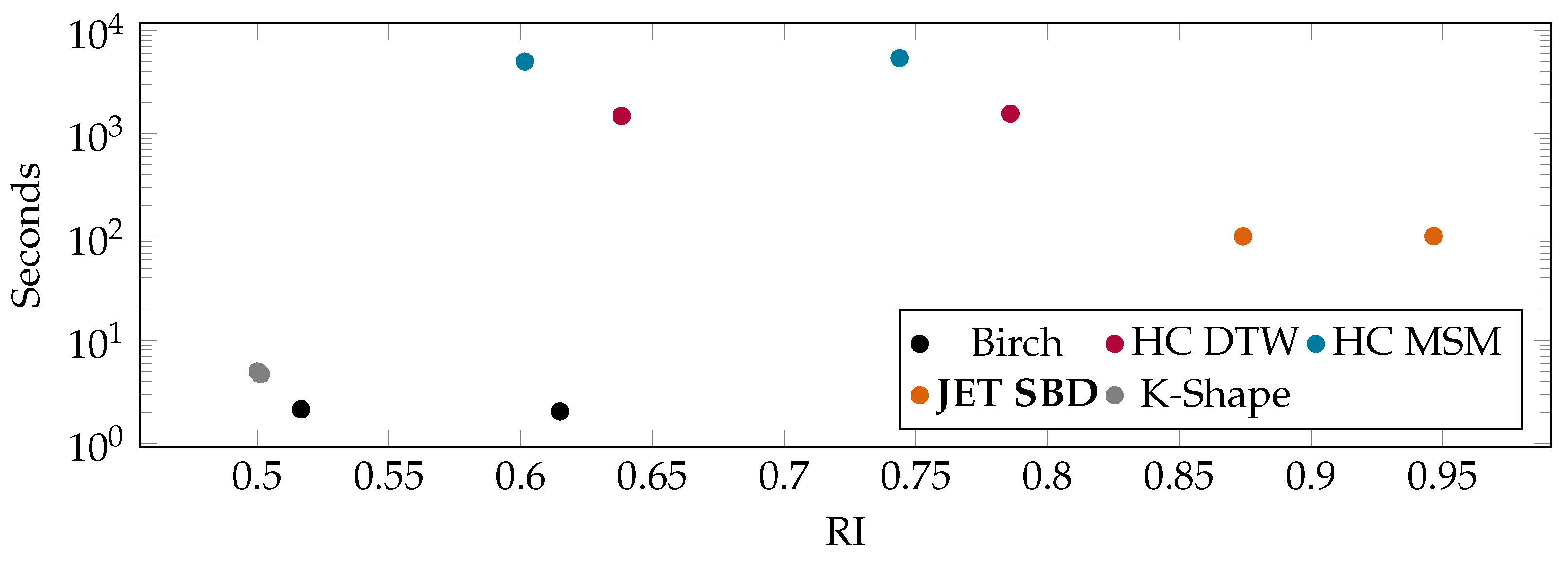
  • Performance and Quality Evaluation of JET: We demonstrate the applicability of popular algorithms to time series clustering and report on the quality and runtime on well-known datasets. The evaluation shows that JET outperforms similarly accurate state-of-the-art approaches in runtime and similarly efficient approaches in accuracy (Section 6).

2. Advancing Jet Engine Development

The JET algorithm was developed for a practical use case in collaboration with our industry partner Rolls-Royce, which is a leading provider of power and propulsion systems.
One of its main businesses is the development of modern jet engines, which is a complex, expensive and long process that involves a variety of challenges. These challenges include ensuring the engine is safe and reliable, meeting performance and environmental requirements, and at the same time, keeping costs and schedules under control. Physical tests play an important role in the development process as they validate product designs against these requirements. Executing the tests, though, presents various challenges, many of which are related to managing and analyzing large amounts of data. Time Series Anomaly Classification is a powerful tool for engineers to quickly detect and diagnose abnormalities in test data sets. It can provide valuable insights and aid in root cause analysis by classifying detected anomalies into categories, such as unintended bleed air leakage, bleed air contamination, or engine misfire. This gives engineers more control over their hardware, as they can identify potential issues before they result in costly failures of equipment or components. With the evolution of sensor technology and the development of more precise and modern test beds, state-of-the-art clustering algorithms have become a bottleneck in this process. The proposed clustering algorithm, JET, was therefore developed to accelerate the clustering process with hardly any compromises on accuracy.

3. Related Work

In order to cluster detected anomalies (or any other kind of time series collection) into similar groups, we consider clustering algorithms that can work with time series data. Most clustering algorithms rely on a certain distance measure, but not all measures are suitable for time series. Our approach, JET, aims to estimate an Agglomerate HC variant. There are already other algorithms that estimate HC to speed up its runtime, but with JET, we propose optimizations that specialize specifically in time series data.

3.1. Clustering Approaches

Many classical clustering approaches, such as K-Means [14], K-Medoids [15], MeanShift [16], DBSCAN [17], and OPTICS [18], were published using Euclidean distance. Unfortunately, this reliance excludes them from analyzing time series anomalies if these have different lengths. Therefore, several time series clustering algorithms have been suggested with different time series distance measures. For example, K-Means [19] can use Dynamic Time Warping [20] (DTW) and K-Shape can use Shape-Based Distance [21] (SBD) to generate the distance between two time series. The mentioned approaches and other clustering techniques that can process time series of arbitrary length either scale badly, are too inaccurate, or do not fit our industry setting.
Birch [22] is a clustering approach that builds a data hierarchy to group data points with the Clustering Feature (CF) heuristic. A CF is a tuple of three values ( N , L S , S S ) , where N is the number of data points a CF group contains, L S is the element-wise sum of the data points, and S S is the squared sum. The algorithm generates a CF-Tree that represents a hierarchy of groups used to cluster the data. Birch is developed to cluster large amounts of data in a short time. However, its reliance on element-wise calculations prohibits it from clustering time series of different lengths. Anyhow, by first embedding the time series, our approach can use Birch for highly efficient, feature-based pre-clustering.
The Time2Feat [23] approach calculates features for time series and clusters the data based on these features. In this way, it transforms the time series into a uniform format with which Euclidean distances can be calculated. Although Time2Feat cannot handle time series of varying lengths, JET also uses the concept of transforming time series into features to create fixed-size time series representations.
Agglomerate HC [24] is a special approach that requires only a distance matrix of all points in a data set. From the bottom up, it merges data points and generated clusters that are closest to each other. Agglomerate HC can use several different techniques, known as linkage methods, to calculate the distance between two clusters: For example, single uses the distance between the two closest members, complete sums up all distances of all members, and Ward [25] considers the change in summed squared distances after merging to be the distance. The clustering algorithm’s runtime for calculating the distance matrix, however, grows quadratically with the size of the dataset and, thus, the algorithm becomes impossible to use after a certain data size is reached. Of note, the distance matrix can be calculated with distance measures from the similarity between time series of different lengths [26]. Due to its quadratic runtime, several approximation approaches for HC have been proposed. HappieClust [27], for example, uses so-called pivots and calculates the distance for each data point to each of the q pivots. In this way, every data point receives new coordinates in a q-dimensional pivot-space. Then, it chooses n random pairs and calculates pseudo-distances between their distance profiles, which are the Chebychev Distance in the pivot space. The pseudo-distances help estimate how many pairs are actually close to each other. The algorithm takes all pairs with a pseudo-distance smaller than the estimated error ϵ to then calculate their real distances. Moreover, it also takes a fraction of random pairs and calculates their real distances, too. Afterwards, HappieClust performs bottom-up hierarchical clustering by using the known distances, which approximate the remaining unknown distances with the help of the Triangular Inequality (TI). TI only works in metric spaces, such as the Euclidean space, and, thus, is suboptimal for time series clustering. Our approach also calculates only a part of the whole distance matrix and estimates the remaining distances based on the already calculated ones. Grinch [28] is another HC approximator and online algorithm that can reconfigure the hierarchy with new data points based on specialized linkage functions. Grinch requires a labeled dataset to find good partitioning and, hence, does not solve our unsupervised clustering task.
In summary, our unsupervised clustering approach, JET, uses HC with Ward linkage and the SBD distance measure to cluster time series, but estimates the distance matrix with Birch, which pre-clusters the time series based on their features, to compensate for the long runtime. We demonstrate that this optimization makes the otherwise costly hierarchical clustering of variable-length time series possible.

3.2. Distance Measures

The distance between two time series cannot be calculated with Euclidean distance if they are, as in our business’s case, of different length. Because our anomaly time series are approximate cut-outs of larger time series, similar time series are also often shifted, such that position x in one time series logically corresponds to some position x + y in another time series. Lockstep measures, which compare time series point-wise like Euclidean distance, cannot capture these matches.
The Dynamic Time Warping [20] (DTW) measure is an edit distance that finds mapping between two time series that can be of different lengths or shifted by searching the shortest path in a dynamic programming setting. It maps single points from one time series to a set of contiguous points from the other time series. The more point sets from one time series relate to single points from the other, the more these time series differ from each other. With DTW Barycenter Averaging (DTW) [19], we can generate a representative in the DTW space of a group of time series. DBA iteratively minimizes the sum of Euclidean distances to all time series of a group.
The Move Split Merge [29] (MSM) metric is also an edit distance measure similar to DTW. Instead of mapping a single point to a set of points, MSM can also insert, move, or delete values in order to make one time series resemble the other. The more operations are used, the more the time series differ. When calculating the distance with MSM, a parameter is necessary to set the cost for each operation. This parameter behaves differently with varying time series inputs. Hence, MSM is not straight forward to use and optimize, so we opted for SBD in our approach. Also, here, a method to find a representative (or mean) of a group of time series in the MSM space exists. MSM-MEAN [30] uses a ( k + 1 ) -dimensional table (with k as the number of time series in a group), in which a shortest path is found by using dynamic programming.
The Shape-Based Distance [21] (SBD) is the distance measure behind the K-Shape algorithm. It calculates the maximum cross-correlation ( C C ) between two time series that is normalized with the self-dot products of both time series: S B D ( a , b ) = 1 max ( C C ( a , b ) ( a · a ) ( b · b ) ) . This measure slides one time series over the other. For each intersection, it calculates the dot product of both time series and normalizes it with the self-dot products. The maximum value of all sliding positions is considered the similarity measure. Intuitively, the time series are slid over each other until the shapes are most similar. In [26], the proposed transformation from similarity to distance is 1 similarity . For SBD, however, the similarity measure is subtracted from 1 to transform it into a distance measure. With the GRAIL [31] method, we can find a representative of a group of time series in the SBD space. For this purpose, GRAIL detects multiple landmark time series, which it uses to estimate a representation matrix for the group of time series.
In this study, we compare the quality of the three measures DTW, MSM, and SBD and use the best, which is SBD, as the default internal distance measure of our JET algorithm.

4. Jaunty Estimation of Hierarchical Time Series Clustering

This section introduces our HC approximation algorithm JET with its four main steps: feature embedding, pre-clustering, distance matrix estimation, and hierarchical clustering. We illustrate these steps and their tasks in Figure 1.
JET takes two parameters: the number of clusters c that are to be created, and the number of clusters c p r e that the pre-clustering step should use. With c, the user can specify the granularity of the final clustering similarly to other clustering approaches, such as K-Means; the best value for c is use-case-dependent, but thanks to hierarchical clustering, different c values can efficiently be tested once JET has finished the four clustering steps. The parameter c p r e allows the user to trade off runtime and precision; it controls the granularity of pre-clustering such that larger values increase runtime and precision, and lower values decrease both. For the optimal trade-off, a fast runtime, and a good estimation, we set c p r e to 3 n , with n as the number of time series to cluster. The algorithm starts by encoding the time series into a fixed-size embedding space (Section 4.1). JET then clusters these embeddings into c p r e clusters in the pre-clustering step (Section 4.2). With these clusters, it partially calculates and partially estimates the full distance matrix of all time series with reference to some accurate but also expensive length-agnostic distance measure, such as DTW, MSM, or SBD (Section 4.3). Afterwards, JET performs HC on the (partially approximated) distance matrix to produce the final hierarchical clustering (Section 4.4). It is important to note that the pre-clustering does not impose its pre-clusters onto the final hierarchical clustering. The hierarchical clustering is largely independent of the pre-clustering and may therefore choose different groupings based on the distance matrix and its own, more precise distance measure. For example, if exactly calculated distances within pre-clusters are larger than approximated distances between pre-clusters, then the time series pairs from different pre-clusters will merge earlier in the hierarchical clustering than the pairs from the same pre-cluster. The pre-clustering instead defines which pair-wise distances are (a) calculated based on the time series themselves or (b) estimated based on centroids. It introduces some distance approximation for time series that stem from different pre-clusters, which are likely the most dissimilar time series pairs, to improve the runtime significantly. Hence, it controls only the runtime–precision trade-off but not the main hierarchical clustering itself, which uses no embedding and a more elaborate distance measure.
In the following, we introduce the JET algorithm in more detail. For this, we use Algorithm 1 and Figure 1 to illustrate the steps that JET performs to cluster the provided time series. We will refer to these two figures throughout this section.
Algorithm 1: JET
1: procedure JET( D , c , c p r e , F )
2:        n D . l e n g t h
3:        e n c z e r o M a t r i x ( n ) Section 4.1
4:       for  i   in   [ 0 , D . l e n g t h [  do
5:             for  f   in   [ 0 , F . l e n g t h [  do
6:                    e n c [ i , f ] F [ f ] . e x t r a c t ( D [ i ] )
7:        p r e A n n o t a t i o n s b i r c h ( e n c , c p r e ) Section 4.2
8:        d m f u l l z e r o M a t r i x ( n , n ) Section 4.3
9:        d m c e n t r o i d s z e r o M a t r i x ( c p r e , c p r e )
10:       p r e G r o u p s u n i q u e ( p r e A n n o t a t i o n s )
11:      for  i   in   [ 0 , c p r e [  do▹ Centroid Distance Matrix
12:             c e n t r o i d i g e t C e n t r o i d ( p r e G r o u p s [ i ] )
13:            for  j   in   [ i + 1 , c p r e [  do
14:                   c e n t r o i d j g e t C e n t r o i d ( p r e G r o u p s [ j ] )
15:                   d m c e n t r o i d s [ i , j ] d ( c e n t r o i d i , c e n t r o i d j )
16:                   d m c e n t r o i d s [ j , i ] d m c e n t r o i d s [ i , j ]
17:      for  i   in   [ 0 , n [  do ▹ Full Distance Matrix
18:             g r p i p r e A n n o t a t i o n s [ i ]
19:            for  j   in   [ i + 1 , n [  do
20:                    g r p j p r e A n n o t a t i o n s [ j ]
21:                   if  g r p i = = g r p j  then
22:                           d m f u l l [ i , j ] d ( D [ i ] , D [ j ] )
23:                           d m f u l l [ j , i ] d m f u l l [ i , j ]
24:                   else
25:                           d m f u l l [ i , j ] d m c e n t r o i d s [ g r p i , g r p j ]
26:                           d m f u l l [ j , i ] d m f u l l [ i , j ]
27:       l a b e l s w a r d L i n k a g e ( d m f u l l , c ) Section 4.4
28: return l a b e l s

4.1. Feature Embedding
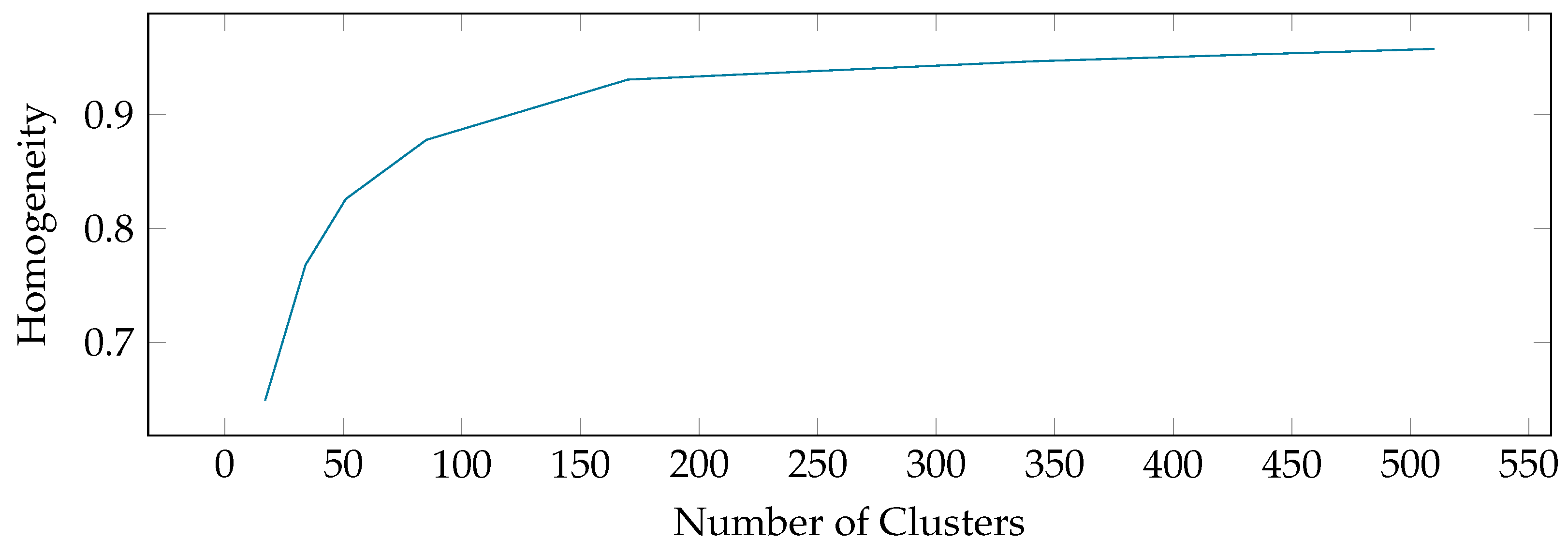
Clustering approaches that can handle time series of different lengths have longer runtimes and higher computational complexity than clustering algorithms for same-length time series. For this reason, our aim is to use a fast clustering algorithm, such as K-Means or Birch, for pre-clustering and to, in this way, support a slower but more accurate hierarchical clustering algorithm afterwards. Because these fast algorithms can handle only fixed-size data, we must first transform the time series in a fixed-size embedding space. For this transformation, JET collects a large number of features for every time series in the input dataset (Lines 3–6 in Algorithm 1). The features cover properties such as time series length, variance, mean etc., and model one dimension in the embedding space each. In this way, every time series has the same number of features, i.e., dimensions in the embedding space (see blue matrix in Figure 1). In this space, JET can calculate Euclidean distances and other distance metrics based on same-lengths inputs. To ensure the same weights for all features, our approach z-normalizes the features as a downstream step.
For feature extraction, JET uses the tsfresh [32] library. This Python tool can extract a large number of time series features with little effort. Its collection ComprehensiveFCParams (https://github.com/blue-yonder/tsfresh/blob/d059eeca6dae80832600ec64a43d941caf746862/tsfresh/feature_extraction/settings.py#L133, accessed on 3 July 2024) includes 386 unique time series features. For the selection of the most important features, we ran Bayesian optimization on one of our industry partner’s datasets with two labeled clusters. The optimization’s objective was to maximize the homogeneity score [33] of a much higher number (60) of clusters found by Birch. The homogeneity score evaluates how many data points of differently labeled clusters appear together in the same cluster. The optimizer ended up with 190 features and removed those that were harmful to the homogeneity of the resulting clusters. We fixed the remaining 190 features as JET’s default embedding features, such that JET uses them for all input datasets. If annotated training data are available, one could fine-tune JET’s feature selection, but JET primarily targets unsupervised clustering tasks, and the static feature selection already shows very good and reliable results (see Section 6.2).

4.2. Pre-Clustering

Our goal is to estimate large parts of the distance matrix with already pre-clustered groups using the centroids of these groups as surrogates for the distance calculations. For this, the distances of time series from different pre-clusters need to be as similar as possible to the distances of their respective cluster centroids. To ensure proper estimations, time series that belong to different clusters should also not be in the same pre-clusters. Thus, the homogeneity [33] of the pre-clustering should be very high. The homogeneity of clusters grows with an increasing number of clusters. The most extreme case is having as many clusters as data points and every data point being its own cluster. Then, we have a 100% homogeneity. On the flip side, having all data points, i.e., time series, in one cluster results in the lowest homogeneity. Figure 2 shows the increasing homogeneity with an increasing number of clusters that the Birch algorithm generates on a sample dataset.
JET can exploit this fact by clustering the feature-space-embedded data from Section 4.1 with a much higher number of clusters c p r e than demanded for the end result c. Birch [22] is the fastest among the tested clustering algorithms and yields good results with a large c p r e as the input parameter. Therefore, we use it as a pre-clusterer (Line 7 in Algorithm 1).

4.3. Distance Matrix Estimation

To perform HC with Ward linkage in the last step, JET requires a distance matrix of all points, i.e., time series, in the dataset. This requirement is expensive, because the time for calculating a full distance matrix grows quadratically with the number of time series. To speed up this calculation, we must first understand how the Ward linkage algorithm for time series works.
HC algorithms merge clusters iteratively accoriding to a linkage method, which defines the cluster distances based on the previously computed distance matrix. For each step of an HC algorithm, the two closest clusters are merged to a new cluster. If the algorithm has not built clusters yet and every data point is its own cluster, the two closest data points are merged. If the merging involves already generated clusters C i and C j , Ward linkage calculates the summed squares of all distances in C i as S S D ( C i ) and in C j as S S D ( C j ) . Then, it calculates the summed squares of the combined cluster C i + j as S S D ( C i + j ) . The difference in the summed squares of C i and C j with C i + j is considered the distance between both clusters: S S D ( C ) = ( c x , c y ) C × C S B D ( c x , c y ) 2 and W a r d ( C i , C j ) = S S D ( C i + j ) ( S S D ( C i ) + S S D ( C j ) ) . Sometimes, Ward linkage is referred to as min-variance linkage, because the summed squared distances correlate with the variance of all distances in a cluster. Here, Ward checks how much the variance of distances changes after merging two clusters. To find the new variance, Ward must know all distances (e.g., S B D ) within the clusters C i and C j , and the distances of all time series from C i to the time series in C j .
If the convex hulls of two clusters have no or only a few intersections, the mean distance between the elements of C i and the elements of C j is close to the distance between the centroids of both clusters. Hence, we can use the centroid distance to estimate the distances between any point in C i to any point in C j . When Ward calculates the new variance of distances in C i j , it does not need to calculate all distances between C i and C j , but instead, takes the centroid distances as an estimate.
For the actual calculation/estimation of the distance matrix, from which Ward pulls the distances in each step, we use the groupings from the pre-clustering in Section 4.2, that partitions our input dataset into groups of similar time series. For every group, we calculate its full and precise distance matrix (c.f. green boxes along the diagonal in Figure 1) according to one of the previously mentioned distance measures (DTW, MSM, or SBD). Then, we insert the distance matrices of the groups to their respective spots in our full distance matrix and leave the rest blank (Lines 22–23 in Algorithm 1). The more groups, i.e., pre-clusters, we have, the sparser our full distance matrix and the more inexpensive the precise distance calculations become. JET also calculates a distance matrix of all centroids of the pre-cluster groups (Line 11 in Algorithm 1). The empty spots in the full distance matrix are then filled with the distances between the pre-cluster centroids in the full distance matrix. The estimated distance between two points is the distance between the centroids of their assigned groups (Lines 25–26 in Algorithm 1). As an example, the solid green value in Figure 1 corresponds to the distance between the second and sixth time series and is estimated by taking the centroid distance of their respective pre-clusters, which are the boxes both arrows originate from. In this way, we can generate a full distance matrix that requires less computation than calculating all distances.
As mentioned in Section 4.1, distance measures in time series clustering might need to deal with varying time series lengths. These cases prevent the use of lockstep distances, such as Euclidean distance, for the calculation or estimatation of distances in the matrices. Elastic distance measures, such as DTW, SBD, and MSM, however, can be used to calculate distances between time series of different lengths, and are therefore all supported in JET.
To measure the distance between two clusters, we could either calculate a mean time series for each cluster or select a medoid time series from the cluster’s members. Because calculating a mean time series for a centroid is often not feasible (due to the time series’ heterogeneity) or too expensive (due to the time series’ sizes) [19,30,31], JET selects the medoid time series of each cluster as its centroid. The medoid time series of a cluster is the cluster member, whose sum of distances to the remaining cluster members is minimal.

4.4. Hierarchical Clustering

In the last step, JET takes the partially calculated and partially estimated distance matrix (Section 4.3) to perform a standard hierarchical clustering approach with Ward linkage (Line 27 in Algorithm 1). The output of the final clustering step is a dendrogram that JET cuts down to the c requested clusters. A user can, of course, interactively define any number of clusters without re-executing the entire clustering, which is for many exploratory use cases a practically highly relevant feature for clustering (besides high accuracy and low runtime).

5. Theoretical Runtime Analysis

The most expensive task of an HC algorithm is the calculation of the distance matrix of all n data points, especially when clustering large time series. Its runtime grows quadratically with n. Because the distance matrix is mirrored on its diagonal, in practice, only about half of it must be calculated. Hence, the exact HC approach has a runtime of n ( n 1 ) 2 distance calculation for the distance matrix. Our approximating JET approach pre-clusters the n data points into c p r e = 3 n groups, which provides a good trade-off between the number and size of groups. With a c p r e = n , there are as many groups as there are members on average, and it has the fewest distance calculations. With a higher number, we obtain more distance calculations, but can counter Birch’s bad quality even more. In the best case, Birch uniformly assigns each of these groups m = n 3 n members. For each group, we then have to calculate m ( m 1 ) 2 distances, which results in a total of 3 n m ( m 1 ) 2 = n ( n 3 1 ) 2 distances. The calculation of the centroids’ distances for the full distance matrix requires another 9 n 3 n 2 calculations, because we have 3 n groups. Hence, the total number of distance calculations is n ( n 3 + 8 ) 3 n 2 . Compared to the exact approach, this is a speedup of n 1 n 3 + 8 3 n n . However, this is the best case scenario. In most cases, the pre-clustering does not uniformly assign the data points to groups. In the worst (but unlikely) case, JET assigns only one data point to 3 n 1 groups each and the rest of the n ( 3 n 1 ) points to one group. Then, the number of distance calculations would be n ( n 6 n + 19 ) 6 n 2 . Still, this would be a speedup of n 1 n 6 n + 19 6 n n , which is close to but still better than the exact HC’s runtime. Figure 3 visualizes the number of distance calculations for different numbers of data points n and the theoretical potential of our new approach. In Section 6, we report actual runtime measurements on different benchmark datasets.

6. Experimental Evaluation

In this section, we evaluate the efficiency and performance of JET for the clustering of time series. Our experiments evaluate the measurements taken from nine state-of-the-art clustering algorithms and JET with different distance measures for time series datasets from the UCR Time Series Classification Archive (Section 6.2). We also compare the performance of JET to the performance of its competitors on two real-world datasets from our industry partner and evaluate the algorithms’ applicability to real-world scenarios (Section 6.3).

6.1. Experimental Setup

To assess the quality of the produced clusterings, we measure the Rand Index (RI) [34] for each clustering. The RI calculates the ratio of pair-wise correctly grouped time series and all pairs of time series. A pair of time series is considered correct if this pair is clustered together and it is also in the same ground truth cluster. Hence, the RI score is a floating point accuracy value between 0 (no correct pairs) and 1 (all correct pairs) that is independent of actual class names.
We compare the performance of JET with 14 competing approaches. Some of these algorithms (K-Means Euclidean, DBSCAN, HappieClust, MeanShift, OPTICS, Birch) require datasets with time series of the same length; for their testing on variable lengths of corpora, we compress the time series to the size of the smallest time series per dataset. The other algorithms (K-Medoids, K-Means DTW, K-Shape, JET, HC) can cope with varying time series lengths and therefore always receive the original time series as an input. We use the default parameters for all algorithms and set the number of clusters c for each algorithm to the expected number of clusters, except for MeanShift, which finds this number on its own. The cost parameter for the MSM distance measure is set to 700, because this setting yielded the most robust results in our experiments.
All experiments use Python implementations of JET and its competitors for a fair runtime evaluation. We published the code for JET and all experiments on GitHub (https://github.com/HPI-Information-Systems/jet, accessed on 3 July 2024). We also developed a Python library called Tidewater (https://github.com/HPI-Information-Systems/tidewater, accessed on 3 July 2024) to build data pipelines and perform the experiments that are reported in this section. Our experiments were run on a server with an Intel Xeon E5-2630 v4 CPU with 20 threads and 60 GB RAM. The JET algorithm can, however, easily run on a consumer PC as well due to its small resource requirements.
To assess JET’s and the other algorithms’ quality, we used datasets from the UCR Time Series Classification Archive [35]. Because JET focuses specifically on variable-length time series collections, we partitioned the UCR datasets into datasets with varying lengths (AllGestureWiimoteX, AllGestureWiimoteY, AllGestureWiimoteZ, GestureMidAirD1, GestureMidAirD2, GestureMidAirD3, GesturePebbleZ1, GesturePebbleZ2, PickupGestureWiimoteZ, PLAID, and ShakeGestureWiimoteZ) and the remaining datasets with only fixed lengths and evaluated these collections separately. For the assessment of the algorithms’ applicability to real-world data, we used two time series datasets provided by our industry partner Rolls-Royce. For security and legal reasons, we cannot publish these datasets, but report their meta-data and the results of JET and other algorithms (Section 6.3).

6.2. Benchmarks on Publicly Available UCR Data

Our first experiment evaluates the quality and runtime of JET and its competitors on the UCR Archive. Figure 4 plots the RI clustering scores for the different clustering algorithms with the different distance measures for the varying-length and equal-length datasets, respectively. The results show that HC with SBD actually has the highest median RI on the datasets containing time series with varying lengths. Our JET algorithm with SBD, which approximates the exact HC, is only slightly worse than HC, and is therefore the second best algorithm. Because JET is always very close to the exact HC independently of the distance measure, we conclude that JET qualitatively succeeds in being a good estimation of HC. The third (K-Medoids SBD) and fifth (K-Shape) best algorithms also utilize the SBD distance measure. Other distance measures, such as DTW and MSM, still yield acceptable results, but systematically worsen the RI score in comparison to SBD. Hence, we also conclude that SBD is qualitatively the best distance measure for our evaluation set. With large variance but a relatively high median RI score, Birch managed to be the fourth best algorithm in our experiments on varying lengths of time series. This shows that Birch can actually achieve decent clustering results given our feature embeddings; hence, it is an effective pre-clustering component in JET. We also evaluated all algorithms on the equal-length datasets. The results in Figure 4 (right) show that most algorithms achieve (on average) comparable clustering RI scores. The scores for equal-length time series are, on average, worse than the scores for varying-length time series, because these clustering datasets happened to be of the higher difficulty. K-Shape reaches the highest median RI of 0.735 ; the best HC variant HC DTW reaches a median RI of 0.705 ; and the corresponding JET algorithm reaches a slightly higher median RI of 0.706 . These results again show that JET also approximates HC very well on time series datasets with equal lengths, although equal-length time series are not our main objective. The fixed-length clustering algorithms, which had to cluster compressed time series data on the datasets with varying time series lengths, clearly performed worse than the variable-length clustering algorithms; some of them even performed poorly on equal-length datasets. The five worst algorithms had RI scores below 40% and are therefore not considered for our further runtime experiments.
K-Means with DTW is, as shown in Figure 5 (left), the slowest among all the algorithms. This might, however, be due to the implementation details of the K-Means tslearn [36] implementation, which can handle time series data with varying lengths better than other libraries, because the very similar K-Medoids algorithms perform much better here. The runtime is still so much worse than all other runtimes that the implementation details alone cannot explain it. Figure 5 (left) shows that calculating an exact and complete SBD distance matrix also takes a long time. Both HC with SBD and K-Medoids with SBD rely on a full distance matrix. Hence, their runtimes are the longest runtimes of all algorithms. JET with SBD only approximates certain parts of the distance matrix (with the cluster centroids) and is therefore significantly faster than all HC variants, especially with SBD. Birch is the fastest algorithm, followed by K-Shape. Both of these super-fast algorithms do, however, perform worse than JET in terms of RI score on varying-length time series. JET is among the fastest clustering approaches in the experiment and can therefore meet practical execution time limits.
In Section 5, we discussed the theoretical lower- and upper-bound runtimes of JET and compared them to the runtime of the exact HC approach. In Figure 5 (right), we plot the results for different numbers of time series in the datasets and observe that JET’s average case runtime is closer to its lower theoretical bound and far from its upper bound. HC SBD’s runtime is considerably higher than JET’s runtime. The other variants of HC use different distance measures that are faster to compute. Thus, the approximation of JET is less impactful and its runtimes therefore differ less from the other runtimes. Note that on the datasets with 700 time series, the faster algorithms experience a (slightly) decreased runtime, because the time series in these datasets are on average shorter than time series in the smaller datasets.
The experiments on the UCR Archive show that JET is among the most accurate clustering algorithms for varying-length datasets, with only very small approximation errors. Its runtime is clearly superior to the runtime of the exact HC, especially when used with the distance measures SBD and MSM, which work particularly well for varying-length time series. In comparison to all state-of-the-art clustering algorithms, JET outperforms similarly accurate competitors in runtime and similarly efficient competitors in accuracy.

6.3. Benchmarks on Rolls-Royce Industry Data

For the industry evaluation, we choose only the five best algorithms from Section 6.2 that are also among the fastest: JET SBD, Birch, K-Shape, HC DTW, and HC MSM. The task is to cluster two datasets in which both clusters of time series have varying lengths. The datasets contain around 7000 time series each. These time series constitute automatically detected anomalies and have an average length of about 30 time steps. Figure 6 shows that JET with the SBD distance measure is the most accurate algorithm in this experiment, because HC SBD was simply too slow for this experiment (stopped after 10× the time of JET). JET’s RI scores are 88% and 94%, respectively. JET’s runtimes are also orders of magnitude faster than the HC variants’ runtimes. Although Birch and K-Shape are even faster than JET, their clustering quality is too low to be considered useful for this time series clustering use case. Both performance characteristics, the improved clustering quality and runtime, allow our industry partner to accelerate the development of jet engines, because JET can group large amounts of time series anomalies reliably in a practically acceptable time (about 100 s for 7000 detected anomalies). The generated clusters and representatives thereof can be shown to an engineer with deeper domain knowledge to quickly categorize the observations. The engineer can also refine the hierarchical clustering by drilling down in the dendrogram to find more fine-grained clusters and, eventually, completely new types of anomalies without re-executing JET.

7. Conclusions

The proposed JET algorithm estimates a hierarchical clustering of a set of time series with the SBD distance measure and Ward linkage. Our theoretical and practical evaluations have shown that JET is up to orders of magnitude faster but still similarly accurate to the exact HC algorithms. Compared to all state-of-the-art clustering approaches, JET either produces clustering results of much better quality or it offers much faster runtimes. All presented clustering methods are offline techniques that can be applied only after an engine test is completed. An even more helpful tool would be an online clustering approach that already raises alerts about anomalies and their types during a test run. Therefore, in future work, we plan to investigate how to extend JET to run online as a streaming algorithm; due to the two-phased approach of JET, we are currently working on a mini-batching technique. Moreover, we aim to scale JET to even larger datasets by developing a distributed version; this distribution could exploit the pre-clustering of Birch for optimal distributed partition management.

Author Contributions

Conceptualization, P.W., T.P. and M.H.; methodology, P.W. and T.P.; software, P.W.; validation, resources, data curation, visualization, writing, P.W., T.P. and M.H. All authors have read and agreed to the published version of the manuscript.

Funding

This work was funded by the German government as part of the LuFo VI call I program (Luftfahrtforschungsprogramm) under grant number 20D1915.

Institutional Review Board Statement

Not applicable.

Informed Consent Statement

Not applicable.

Data Availability Statement

The original data presented in the study are openly available in UCR Time Series Classification Archive at [35] and at https://github.com/HPI-Information-Systems/jet.

Conflicts of Interest

The management of Rolls-Royce Deutschland Ltd. & Co. KG is gratefully acknowledged for supporting this work and permitting the presentation of our results.

References

  1. Ansari, S.; Farzaneh, N.; Duda, M.; Horan, K.; Andersson, H.B.; Goldberger, Z.D.; Nallamothu, B.K.; Najarian, K. A Review of Automated Methods for Detection of Myocardial Ischemia and Infarction Using Electrocardiogram and Electronic Health Records. IEEE Rev. Biomed. Eng. 2017, 10, 264–298. [Google Scholar] [CrossRef] [PubMed]
  2. Woike, M.; Abdul-Aziz, A.; Clem, M. Structural health monitoring on turbine engines using microwave blade tip clearance sensors. In Proceedings of the Smart Sensor Phenomena, Technology, Networks, and Systems Integration 2014, San Diego, CA, USA, 10–11 March 2014; Volume 9062, pp. 167–180. [Google Scholar] [CrossRef]
  3. Cheng, H.; Tan, P.N.; Potter, C.; Klooster, S. Detection and Characterization of Anomalies in Multivariate Time Series. In Proceedings of the SIAM International Conference on Data Mining (SDM), Sparks, NV, USA, 30 April–2 May 2009; pp. 413–424. [Google Scholar] [CrossRef]
  4. Braei, M.; Wagner, S. Anomaly Detection in Univariate Time-series: A Survey on the State-of-the-Art. arXiv 2020, arXiv:2004.00433. [Google Scholar]
  5. Blázquez-García, A.; Conde, A.; Mori, U.; Lozano, J.A. A Review on Outlier/Anomaly Detection in Time Series Data. arXiv 2020, arXiv:2002.04236. [Google Scholar] [CrossRef]
  6. Chandola, V.; Banerjee, A.; Kumar, V. Anomaly Detection: A Survey. ACM Comput. Surv. 2009, 41, 1–58. [Google Scholar] [CrossRef]
  7. Schmidl, S.; Wenig, P.; Papenbrock, T. Anomaly Detection in Time Series: A Comprehensive Evaluation. In Proceedings of the VLDB Endowment, Sydney, Australia, 5–9 September 2022. [Google Scholar]
  8. Malhotra, P.; Vig, L.; Shroff, G.; Agarwal, P. Long short term memory networks for anomaly detection in time series. In Proceedings of the European Symposium on Artificial Neural Networks, Computational Intelligence and Machine Learning (ESANN), Bruges, Belgium, 22–23 April 2015. [Google Scholar]
  9. Ryzhikov, A.; Borisyak, M.; Ustyuzhanin, A.; Derkach, D. Normalizing flows for deep anomaly detection. arXiv 2019, arXiv:1912.09323. [Google Scholar]
  10. Boniol, P.; Palpanas, T. Series2Graph: Graph-Based Subsequence Anomaly Detection for Time Series. Proc. VLDB Endow. 2020, 13, 1821–1834. [Google Scholar] [CrossRef]
  11. Zhu, Y.; Zimmerman, Z.; Senobari, N.S.; Yeh, C.C.M.; Funning, G.; Mueen, A.; Brisk, P.; Keogh, E. Matrix Profile II: Exploiting a Novel Algorithm and GPUs to Break the One Hundred Million Barrier for Time Series Motifs and Joins. In Proceedings of the International Conference on Data Mining (ICDM), Barcelona, Spain, 12–15 December 2016; pp. 739–748. [Google Scholar] [CrossRef]
  12. Bianco, A.M.; Ben, M.G.; Martínez, E.J.; Yohai, V.J. Outlier Detection in Regression Models with ARIMA Errors Using Robust Estimates. J. Forecast. 2001, 20, 565–579. [Google Scholar] [CrossRef]
  13. Hochenbaum, J.; Vallis, O.S.; Kejariwal, A. Automatic Anomaly Detection in the Cloud Via Statistical Learning. arXiv 2017, arXiv:1704.07706. [Google Scholar]
  14. MacQueen, J. Some Methods for Classification and Analysis of Multivariate Observations. In Proceedings of the Fifth Berkeley Symposium on Mathematical Statistics and Probability, Berkeley, CA, USA, 21 June–18 July 1965 and 27 December 1965–7 January 1966; University of California Press: Berkeley, CA, USA, 1967. [Google Scholar]
  15. Kaufman, L.; Rousseeuw, P.J. Partitioning around medoids (program pam). Find. Groups Data Introd. Clust. Anal. 1990, 344, 68–125. [Google Scholar]
  16. Cheng, Y. Mean shift, mode seeking, and clustering. IEEE Trans. Pattern Anal. Mach. Intell. 1995, 17, 790–799. [Google Scholar] [CrossRef]
  17. Ester, M.; Kriegel, H.P.; Sander, J.; Xu, X. A density-based algorithm for discovering clusters in large spatial databases with noise. In Proceedings of the International Conference on Knowledge Discovery and Data Mining, Portland, OR, USA, 2–4 August 1996. [Google Scholar]
  18. Ankerst, M.; Breunig, M.M.; Kriegel, H.P.; Sander, J. OPTICS: Ordering points to identify the clustering structure. ACM Sigmod Record 1999, 28, 49–60. [Google Scholar] [CrossRef]
  19. Petitjean, F.; Ketterlin, A.; Gançarski, P. A global averaging method for dynamic time warping, with applications to clustering. Pattern Recognit. 2011, 44, 678–693. [Google Scholar] [CrossRef]
  20. Berndt, D.J.; Clifford, J. Using dynamic time warping to find patterns in time series. In Proceedings of the KDD Workshop, Seattle, WA, USA, 31 July–1 August 1994; Volume 10, pp. 359–370. [Google Scholar]
  21. Paparrizos, J.; Gravano, L. k-shape: Efficient and accurate clustering of time series. In Proceedings of the 2015 ACM SIGMOD International Conference on Management of Data, Melbourne, VIC, Australia, 31 May–4 June 2015; pp. 1855–1870. [Google Scholar]
  22. Zhang, T.; Ramakrishnan, R.; Livny, M. BIRCH: A new data clustering algorithm and its applications. Data Min. Knowl. Discov. 1997, 1, 141–182. [Google Scholar] [CrossRef]
  23. Bonifati, A.; Buono, F.D.; Guerra, F.; Tiano, D. Time2Feat: Learning interpretable representations for multivariate time series clustering. Proc. VLDB Endow. 2022, 16, 193–201. [Google Scholar] [CrossRef]
  24. Nielsen, F. Hierarchical clustering. In Introduction to HPC with MPI for Data Science; Springer: Cham, Switzerland, 2016; pp. 195–211. [Google Scholar] [CrossRef]
  25. Ward, J.H., Jr. Hierarchical grouping to optimize an objective function. J. Am. Stat. Assoc. 1963, 58, 236–244. [Google Scholar] [CrossRef]
  26. Gower, J.C.; Legendre, P. Metric and Euclidean properties of dissimilarity coefficients. J. Classif. 1986, 3, 5–48. [Google Scholar] [CrossRef]
  27. Kull, M.; Vilo, J. Fast approximate hierarchical clustering using similarity heuristics. BioData Min. 2008, 1, 1–14. [Google Scholar] [CrossRef]
  28. Monath, N.; Kobren, A.; Krishnamurthy, A.; Glass, M.R.; McCallum, A. Scalable Hierarchical Clustering with Tree Grafting. In Proceedings of the 25th ACM SIGKDD International Conference on Knowledge Discovery and Data Mining, KDD ’19, New York, NY, USA, 4–8 August 2019; pp. 1438–1448. [Google Scholar] [CrossRef]
  29. Stefan, A.; Athitsos, V.; Das, G. The move-split-merge metric for time series. IEEE Trans. Knowl. Data Eng. 2012, 25, 1425–1438. [Google Scholar] [CrossRef]
  30. Holznigenkemper, J.; Komusiewicz, C.; Seeger, B. On computing exact means of time series using the move-split-merge metric. Data Min. Knowl. Discov. 2023, 37, 595–626. [Google Scholar] [CrossRef]
  31. Paparrizos, J.; Franklin, M.J. Grail: Efficient time-series representation learning. Proc. VLDB Endow. 2019, 12, 1762–1777. [Google Scholar] [CrossRef]
  32. Blue Yonder GmbH. tsfresh. 2023. Available online: https://github.com/blue-yonder/tsfresh (accessed on 3 July 2024).
  33. Rosenberg, A.; Hirschberg, J. V-measure: A conditional entropy-based external cluster evaluation measure. In Proceedings of the 2007 Joint Conference on Empirical Methods in Natural Language Processing and Computational Natural Language Learning (EMNLP-CoNLL), Prague, Czech Republic, 28–30 June 2007; pp. 410–420. [Google Scholar]
  34. Hubert, L.; Arabie, P. Comparing partitions. J. Classif. 1985, 2, 193–218. [Google Scholar] [CrossRef]
  35. Dau, H.A.; Keogh, E.; Kamgar, K.; Yeh, C.C.M.; Zhu, Y.; Gharghabi, S.; Ratanamahatana, C.A.; Yanping; Hu, B.; Begum, N.; et al. The UCR Time Series Classification Archive. 2018. Available online: https://www.cs.ucr.edu/~eamonn/time_series_data_2018/ (accessed on 3 July 2024).
  36. Tavenard, R.; Faouzi, J.; Vandewiele, G.; Divo, F.; Androz, G.; Holtz, C.; Payne, M.; Yurchak, R.; Rußwurm, M.; Kolar, K.; et al. Tslearn, A Machine Learning Toolkit for Time Series Data. J. Mach. Learn. Res. 2020, 21, 1–6. [Google Scholar]
Figure 1. The four parts of JET: feature embedding, pre-clustering, distance matrix estimation, and hierarchical clustering.
Engproc 68 00037 g001
Figure 2. Birch’s homogeneity score increases with an increasing number of clusters on a fixed sample dataset.
Engproc 68 00037 g002
Figure 3. Distance calculations for the exact HC and approximating JET.
Engproc 68 00037 g003
Figure 4. Rand Index (RI) scores of all algorithms on the UCR Time Series Classification Archive datasets grouped by datasets of varying lengths (left) and equal lengths (right) and ordered by median RI (on varying lengths).
Engproc 68 00037 g004
Figure 5. (Left): Runtime in seconds of well-performing algorithms (mean RI > 0.5 ) on the UCR varying-length datasets ordered by median RI. (Right): Average runtime in seconds of JET and the standard HC algorithm on the UCR datasets with varying lengths plotted against numbers of time series per dataset.
Engproc 68 00037 g005
Figure 6. Rand Index (RI) scores vs. runtime measurements in seconds (on log scale) for two real-world Rolls-Royce datasets.
Engproc 68 00037 g006
Disclaimer/Publisher’s Note: The statements, opinions and data contained in all publications are solely those of the individual author(s) and contributor(s) and not of MDPI and/or the editor(s). MDPI and/or the editor(s) disclaim responsibility for any injury to people or property resulting from any ideas, methods, instructions or products referred to in the content.

