Optimizing Biogas Power Plants through Machine-Learning-Aided Rotor Configuration ^†

Abstract

The increasing demand for sustainable energy sources has intensified the exploration of biogas power plants as a viable option. In this research, we present a novel approach that leverages machine learning techniques to optimize the performance of biogas power plants through the strategic placement and configuration of rotors within the fermentation vessel. Our study involves the simulation of a diverse range of biogas power plant scenarios, each characterized by varying rotor locations and rotating speeds, influencing the agitation levels of the biogas substrate. The simulation results, encompassing multiple performance metrics, serve as input data for an artificial neural network (ANN). This ANN is trained to learn the intricate relationships between rotor placement, rotor speed, agitation levels, and overall system efficiency. The trained model demonstrates predictive capabilities, enabling the estimation of plant efficiency based on specific rotor configurations. The proposed methodology provides a tool for both optimizing existing biogas power plants and guiding engineers in the design and setup of new facilities. Our model aims to offer valuable insights for engineers in the initial planning stages of new biogas power plants, enabling them to make informed decisions that contribute to sustainable and efficient energy generation.

1. Introduction

Biogas power plants stand at the forefront of sustainable energy solutions, playing a pivotal role in addressing the escalating global demand for renewable energy. Despite their potential, these systems are often set up without a comprehensive scientific understanding of the factors influencing their efficiency [1]. A crucial aspect affecting overall performance is the agitation efficiency within the fermentation vessel. In this research, we aim to investigate and optimize biogas power plants by strategically varying both the rotor location and rotating speeds within the vessel.

The lack of a systematic approach in the setup of biogas power plants often results in suboptimal performance and inefficient energy usage. Annas [1] showed an achievable reduction in power input per substrate volume of up to 5 Wm⁻³. Our proposed tool seeks to provide a scientific framework for engineers involved in both the establishment of new plants and the optimization of existing facilities. By manipulating both rotor location and rotating speeds, and taking into account the efficiency of chosen speeds, our method strives to enhance the agitation efficiency of the biogas substrate, ultimately improving the overall system efficiency and avoiding the danger of dead zones while mixing.

The methodology employed in this work involves the utilization of Computational Fluid Dynamics (CFD) models to simulate diverse biogas power plant scenarios. The primary variables in these simulations include both rotor location and rotating speeds within the fermentation vessel. The simulations continue until a steady flow field is achieved inside the vessel. Subsequently, the degree of agitation is quantified by calculating a mixing score based on achieved flow velocities and the agitator energy consumption.

We employ an artificial neural network. Trained on the data derived from the CFD simulations, the ANN becomes a predictive tool capable of estimating a system’s agitation efficiency based on said relevant setup metrics. Considering a rotor’s energy consumption at the respective rotating speeds in our investigation, we hypothesize that the overall agitation efficiency of biogas power plants will exhibit a nuanced dependence on both rotor location and rotating speeds within the fermentation vessel. Striking a balance between low rotating speeds to conserve energy and high rotating speeds to achieve thorough agitation is a key challenge. We anticipate that configurations with tuned rotating speeds coupled with strategic rotor placement will yield the highest efficiency. The specific optimal combinations of rotor location and rotating speeds, however, remain empirical questions that our research seeks to address through a systematic exploration of diverse scenarios. By illuminating the intricate relationships between rotor placement, rotating speeds, and agitation efficiency, we aim to provide valuable insights into the design and optimization of biogas power plants.

2. Methodology

To evaluate the efficiency of mixing within biogas plant reactors, we conducted a comprehensive series of CFD simulations. These simulations aim to mimic the intricate flow dynamics encountered in a biogas reactor and are instrumental in discerning the optimal rotor placements for improved mixing efficiency.

2.1. Computational Fluid Dynamics Single Case Configuration

The CFD case setup in this work was based on the configurations used in our previous work [2]. This involves defining fluid properties, mesh movements, and boundary conditions, as well as specific conditions such as turbulence models, solver types, and the assumption of fluid compressibility. The CFD simulations in the previous paper [2] were designed to capture the complex flow behavior of non-Newtonian fluids within biogas reactors. The fluid’s rheological properties were modeled to reflect the non-Newtonian nature typically observed in biogas substrates. This was achieved by implementing an Ostwald–deWaele power-law model for non-Newtonian fluids with detailed metrics modeled on those of Fosca Conti et al. [3].

$$\begin{array}{c}\hfill \nu =k{\dot{\gamma }}^{n-1},{\nu }_{min}\le \nu \le {\nu }_{max}\end{array}$$

(1)

with the kinematic viscosity $\nu$, a kinematic consistency factor $k=15.4·{10}^{-3}$ m²s⁻¹, and a power-law index of $n=0.35$, where $n<1$ describes the fluid as shear thinning. The fluid’s kinematic viscosity limits were set to ${\nu }_{min}={10}^{-6}$ m²s⁻¹ and ${\nu }_{max}={10}^{-3}$ m²s⁻¹ to include observations from Šafaric et al. [4]. The simulations aim to compute velocities u in each mesh cell, on which the mixing evaluation is based. Higher fluid velocities favor the sedimentation process [1], correlating with better substrate mixing.

A detailed mesh setup was developed to accurately simulate rotor motion interacting with the fluid. This involves the use of Arbitrary Mesh Interfaces (AMI), which are crucial for handling the rotational movement of the blades in the simulation. The AMI allow the mesh to dynamically adapt to the rotating parts, ensuring that the interaction between the moving rotor and the fluid is captured.

Figure 1 shows a comparison of fluid velocity development over 100 s of agitation time. After an initial boost, the fluid slows down and slowly settles at a steady velocity with a similar magnitude to the initial wave. Figure 1a,b show fluid velocity heavily affected by the rotor movement with the point of measurement directly in front of the rotor (magenta cell in Figure 1a). Figure 1b shows the fluid velocity development over time on each axis and the magnitude. Ux, Uy, and Uz refer to velocities u on the X-, Y-, and Z-axis, respectively. Figure 1c,d show the same measurement on a cell located to the left of the rotor (magenta cell in Figure 1c), in an area not affected nearly as much by the rotor movement.

In this work, a simulation time limit of 30 s was used, which strikes a good balance between the time to reach a steady flow field and the computational overhead required to simulate these results.

2.2. Computational Fluid Dynamics Case Batch

A tool has been developed to efficiently generate multiple CFD cases with several consistent parameters and varied conditions to thoroughly investigate the effects on mixing within the reactor such as:

• Rotor Design: Rotor types can vary widely from plant to plant. In this work, different rotor designs were supported by adding chosen rotor geometries to the simulation case.
• Rotor Speed Variation: Each subsequent batch of simulations explored different rotor speeds. This approach allowed us to analyze the interplay between rotor speed and placement, enhancing our understanding of their collective influence on the reactor’s mixing efficiency.
• Rotor Placement Strategy: The strategic placement of the rotor was systematically varied for each set of simulations, known as a batch. Within each batch, the rotor speed remained constant to isolate the effect of placement on fluid dynamics.

Figure 2a schematically illustrates the multiple strategic placements of the rotor considered for the simulation cases within the biogas reactor. The rotor positions, indicated by numbers for each separate simulation case, were varied systematically across multiple simulation cases to assess their impact on mixing efficiency. The consistent representation of the rotor design across all simulations ensured comparability and validity of the results. Figure 2b shows a single simulation case of one batch with a minimal rotor setup and removed top lid.

2.3. Evaluation Method

The evaluation method was designed to establish an objective measure of mixing efficiency within the reactor. In each CFD case, 30 s were simulated to approximate the velocities in a steady flow field (see Section 2.1). A threshold for minimum fluid velocity, required for adequate agitation, was aimed to reach 0.05 ms⁻¹. Velocities in this order of magnitude are conventionally used in biogas plant evaluations (e.g., in [5,6,7]) despite the lack of a robust scientific foundation. This value was adopted here as a general guideline. For quantitative evaluations, the fluid velocity was used in conjunction with the rotor’s type and rotating speed. A mixing score was calculated for each CFD setup, incorporating fluid velocity. Higher fluid velocities are indicative of better substrate mixing and, thus, potentially enhanced biogas production. The used rotor also plays a vital role in the amount of energy consumed for the agitation process. To account for differences in the rotor, the mixing score was normalized by the energy requirement for the given rotation speeds used in a setup. The plant mixing $s_p$ score is the ratio of cells that experience sufficient agitation, as outlined in Section 2.3, and the total number of cells in a given simulation case.

$$s_p=\frac{N_{cs}}{N_c}$$

(2)

where $N_{cs}$ is the number of cells experiencing sufficient agitation of 5 ms⁻¹, and $N_c$ is the total number of cells within the simulation domain. Using $s_p$ alone would favor higher rotor speeds over a more efficient approach. To emphasize the energy efficiency, energy consumption metrics of the rotor at the given rotating speeds were taken into account. Thus, the plant mixing score was normalized over the rotor’s energy consumption metrics:

$$s_{pn}=\frac{s_p}{r_e\left(v_r\right)}$$

(3)

where $s_{pn}$ denotes the efficiency normalized plant mixing score, and $r_e\left(v_r\right)$ is the energy consumption of the rotor at a given rotating speed $v_r$. These metrics are normally found in the agitators datasheets, e.g., [8,9].

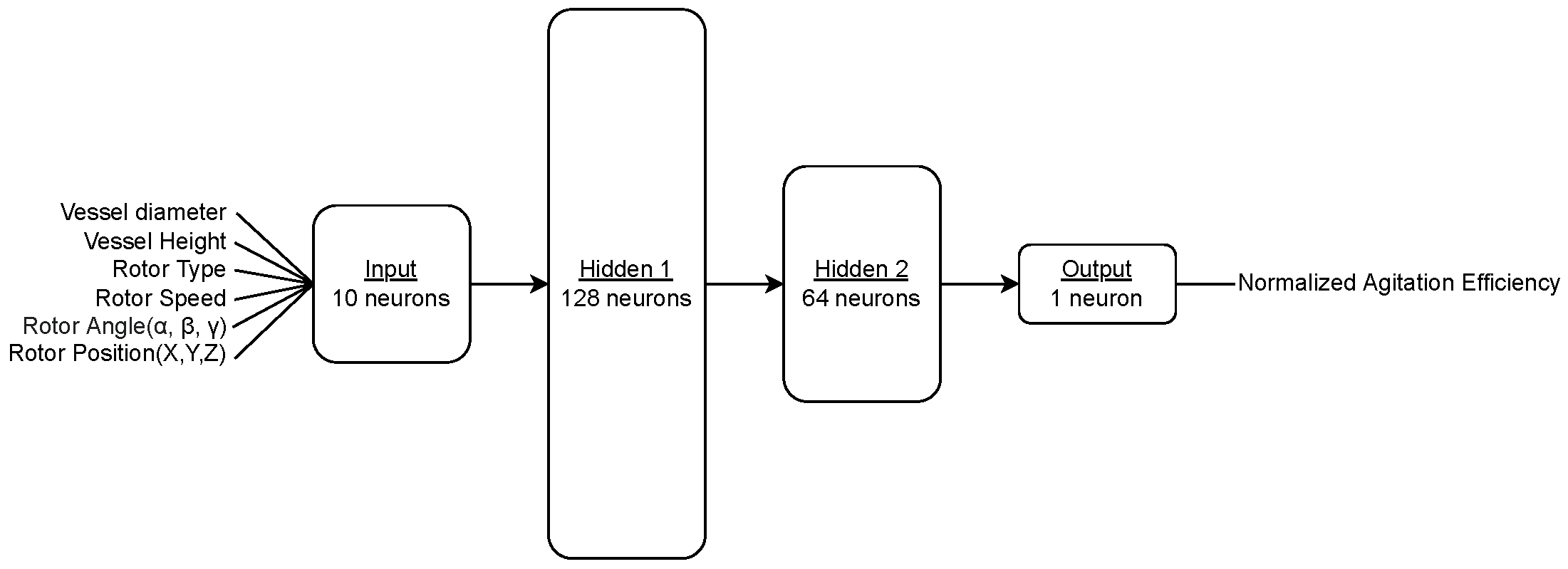
2.4. Shallow Learning

This section details the specific architecture of the neural network used in our shallow learning model, highlighting the structure and functionality of each component.

Figure 3 shows the neural network model architecture used for the regression based recommender model. The model is structured to receive input from ten distinct neurons, each corresponding to a vital parameter that influences the mixing and agitation process within the biogas reactor.

• Vessel Diameter and Height: These parameters define the physical constraints within which the rotors operate.
• Rotor Speed: This is a direct influencer of the agitation intensity within the vessel.
• Rotor Type: Different rotor designs can have significantly different impacts on mixing.
• Rotor Position (X, Y, Z): The spatial positioning of the rotor within the vessel which crucially affects the flow patterns and effective mixing.
• Rotor Angle ($\alpha$, $\beta$, $\gamma$): These angles define the orientation of the rotor, further refining the model’s understanding of how rotors interact with the fluid medium.

The network includes two hidden layers, which are crucial for capturing the nonlinear relationships between the input parameters and the resulting mixing efficiency.

• First Hidden Layer: Consists of 128 neurons. This layer was designed to capture a broad spectrum of features and interactions from the input data. The ReLU activation function is used.
• Second Hidden Layer: Contains 64 neurons. It also uses the ReLU activation function.

The architecture concludes with a single output neuron that employs a linear activation function. The linear activation function allows the model to output a value that directly corresponds to the expected normalized efficiency, as outlined in Section 2.3. The model uses the Adam optimizer. The loss function is the root mean squared error.

2.5. Recommendation

For the recommendation step, the agent is fed with a range of possible solutions, e.g., possible rotor speeds of 7 and 15 rad s⁻¹ and an x-axis position from 0 to 3 m with 1 m resolution. The agent then predicts the Normalized Agitation Efficiency for each set of provided input variables and returns the set of inputs that offered the highest Normalized Agitation Efficiency.

3. Setup

3.1. Simulation Cases

For this work, simulation cases with the following metrics are deployed, with more simulations being processed at the time of submission.

• Vessel Diameter: 10 m;
• Vessel Height: 4 m;
• Rotor Type: Landia POP [8];
• Rotor Speed: 150 RPM and 300 RPM as specified in the rotor datasheet [8];
• Rotor Angle: 0° on each axis;
• Rotor Position: as shown in

  Table 1. Rotor location coordinates within the simulated domains.

  X/m	Y/m	Z/m
  −1	−3	0
  −1	−1	0
  −1	1	0
  −1	3	0
  1	−1	0

  .

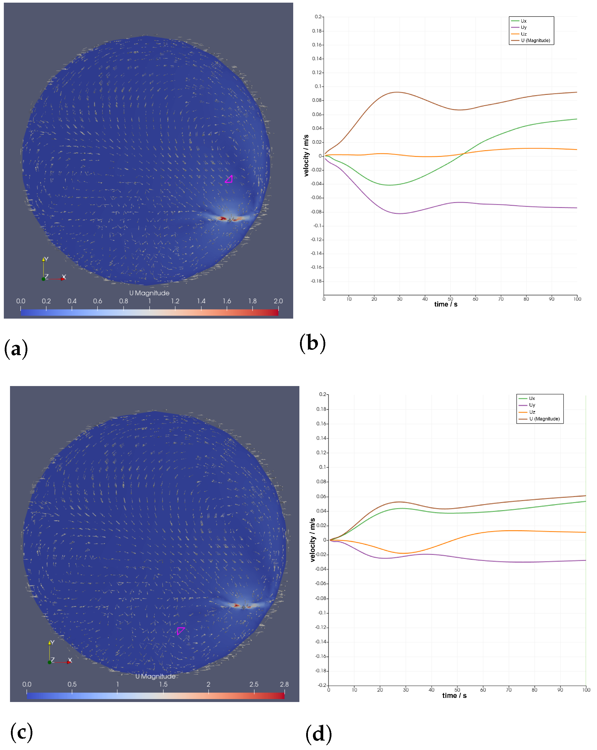
3.2. Computation Post-Processing

Simulations were performed on a cluster provided by FH Münster [10] featuring a total of 20 nodes, each with 24 cores to distribute load across. The load for each simulation case was spread across 12 cores to balance single case simulation times and the number of cases running in parallel. A single case with 30 s of simulation time required around 14 days to complete. The computation was supported by different workstations from the University of Granada.

4. Results

4.1. Training

The shallow learning agent’s training was executed under a supervised learning paradigm, focusing on optimizing the mixing score derived from the previously computed mixing scores outlined in Section 2.3. Each training session processed data in batches of 32 samples across 50 epochs. For the testing of the shallow learning model, the dataset was randomly partitioned into 90% training and 10% testing data, deviating from the more commonly used 80/20 ratio, because of the limited number of training data.

Figure 4 shows the losses of the presented model throughout the training step. After around 35 epochs of training, the models showed signs of overtraining, with the RMSE of the test set dipping way below the performance of the training data, before rapidly recovering. The root cause of this is likely the limited number of training data provided.

4.2. Model Test

As suggested by Figure 4, the system’s ability to accurately estimate the best position was not given. This was validated through an additional test, where the model was fed with the following boundary conditions:

• Vessel Diameter: 10 m;
• Vessel Height: 3 m;
• Rotor Type: Landia POP [8];
• Rotor Angle: 0° on each axis.

The model was then presented with ranges for the rotor speed and position, from which it could choose the best outcome.

• Rotor Speed: Either 7 or 15 rad s⁻¹, which equals around 67 or 143 min⁻¹, respectively.
• Rotor Positions: Possible positions within the cylindrical vessel with 1 m of granularity.

The agent predicted a rotor speed of 15 rad s⁻¹ (around 143 min⁻¹) and a rotor position at X = −3, Y = −3, and Z = 2 m to yield the best result with a Normalized Agitation Efficiency of 5.61 kW s rad⁻¹. This, however, seemed to be above the potential results when compared to the outcome of the simulations, which yielded Normalized Agitation Efficiencies in the range of 3.0 to 3.3 kW s rad⁻¹. The mentioned limitations will likely improve by generating more training data.

5. Discussion

5.1. Model Evaluation

Our current methodology integrates real-world metrics to derive results, aiming to replicate actual operational conditions as closely as possible. The robustness and predictive accuracy of our simulations can only be evaluated with a higher volume of simulated cases. Increasing the number of simulations will allow for a more comprehensive validation of our model across a broader range of scenarios. Metrics taken from the training process indicate a positive development, so providing more training data will certainly improve system performance.

5.2. Mixing Score Evaluation

Our approach to achieving a steady flow field through Computational Fluid Dynamics (see Section 2.1) simulations has demonstrated significant efficacy in predicting the agitation efficiency in biogas power plants. However, an alternative method involving tracking the time it takes for a passive scalar to be transported throughout all cells within the simulation domain was considered. This method could potentially offer more accurate results by capturing the complete mixing time more precisely. Despite its potential for increased accuracy, this approach was deemed not feasible within the scope of our current study due to the extensive computational resources it requires, especially given the high number of simulation cases processed.

5.3. Rotor Angle

The inclusion of rotor angle in the horizontal axes has been a subject of debate. In our cylindrical vessel setup, altering the angle in the horizontal plane does not significantly affect the outcome as it offers a similar result to placing the rotor in a comparable position relative to the vessel’s curvature. This observation suggests that adjustments in the horizontal angle may not be necessary for our current model. However, the angle from the horizontal plane could play a crucial role, a hypothesis that we aim to validate in future studies. This aspect underscores the potential need to refine our model to account for angular influences more effectively.

6. Future Work

6.1. Neural Network

The shallow learning model employed in this study was suitable for the straightforward regression tasks it addressed. Nonetheless, we plan to conduct a more comprehensive analysis of the agent and explore more advanced solutions in future research.

6.2. Training Data

A primary focus for future work is the completion of additional simulations. Our current research has highlighted the importance of extensive simulation data in validating the models and refining their predictive accuracy. By expanding the number of simulation cases, we can enhance the robustness of our findings and better understand the variability and effectiveness of different rotor configurations.

6.3. Comparing to Other Approaches

Currently, many biogas power plant configurations are based on empirical rules of thumb or standardized setups that do not take full advantage of modern analytical tools. Our future research will compare the outcomes and efficiency of the approach outlined in this work.

References

1. Annas, S. Charakterisierung von Rühr- und Mischprozessen in Nicht-Newtonschen Fluiden am Beispiel von Biogasanlagen mit Paddelrührwerk Berichte des Fachgebiets für Strömungsmechanik; Shaker Verlag: Düren, Germany, 2021; ISBN 9783844077827. [Google Scholar]
2. Heller, A.; Glösekötter, P.; Buntkiel, L.; Reinecke, S.; Annas, S. Sim-to-Real Transfer in Deep Learning for Agitation Evaluation of Biogas Power Plants. Eng. Proc. 2023, 39, 69. [Google Scholar] [CrossRef]
3. Conti, F.; Saidi, A.; Goldbrunner, M. Numeric Simulation-Based Analysis of the Mixing Process in Anaerobic Digesters of Biogas Plants. Bioenergy X-Factor 2022, 43, 1522–1529. [Google Scholar] [CrossRef]
4. Šafarič, L.; Yekta, S.S.; Ejlertsson, J.; Safari, M.; Najafabadi, H.N.; Karlsson, A.; Ometto, F.; Svensson, B.H.; Björn, A. A Comparative Study of Biogas Reactor Fluid Rheology—Implications for Mixing Profile and Power Demand. Processes 2019, 7, 700. [Google Scholar] [CrossRef]
5. Shen, F.; Tian, L.; Yuan, H.; Pang, Y.; Chen, S.; Zou, D.; Zhu, B.; Liu, Y.; Li, X. Improving the Mixing Performances of Rice Straw Anaerobic Digestion for Higher Biogas Production by Computational Fluid Dynamics (CFD) Simulation. Appl. Biochem. Biotechnol. 2013, 171, 626–642. [Google Scholar] [CrossRef]
6. Singh, B.; Kovács, K.L.; Bagi, Z.; Nyári, J.; Szepesi, G.L.; Petrik, M.; Siménfalvi, Z.; Szamosi, Z. Enhancing Efficiency of Anaerobic Digestion by Optimization of Mixing Regimes Using Helical Ribbon Impeller. Fermentation 2021, 7, 251. [Google Scholar] [CrossRef]
7. Muninathan, K.; Arivazhagan, S.; Yuvaraj, R.; Madhupriya, K.; Shanmathi, M. CFD Analysis on Performance Improvement of Impeller Mixing Solid Waste in Anaerobic Digestion. In Proceedings of the 2020 International Conference on System, Computation, Automation and Networking (ICSCAN), Puducherry, India, 3–4 July 2020; pp. 1–5. [Google Scholar] [CrossRef]
8. Landia. POP Datasheet. Available online: https://www.landia.de/Files/Images/landia/dataark/Landia_Datenblatt_POP-I.pdf (accessed on 5 May 2024).
9. Landia. POPL Datasheet. Available online: https://www.landia.de/Files/Images/landia/dataark/Landia_Datenblatt_POPL-I.pdf (accessed on 5 May 2024).
10. FH Münster. Campus Cluster index. Available online: https://www.fh-muenster.de/phy/labore/campus-cluster/index.php (accessed on 5 May 2024).
Figure 1. Comparison of fluid velocity development throughout a simulation. The simulation setup and the points of measurement (magenta) are shown in (a,c). The associated velocity developments over time at the respective locations are shown in (b,d).
Engproc 68 00046 g001
Figure 2. (a) Strategic placement of rotors within single case setups of one batch. (b) Model of a single case setup with the rotor placed near the vessel’s wall.
Engproc 68 00046 g002
Figure 3. Fully connected neural network model architecture used in this work. The input layer consists of 10 neurons, followed by two hidden layers with 128 and 64 neurons, respectively, before outputting on one single neuron on the output layer, which describes the estimated Normalized Agitation Efficiency. The Adam optimizer is used, and the activation function of each layer is a Rectified Linear Unit (ReLU), except for the output layer, which has linear activation.
Engproc 68 00046 g003
Figure 4. Root mean square error of training and test sets over 50 training epochs.
Engproc 68 00046 g004