Multi-Objective Optimisation for the Selection of Clusterings across Time ^†

Abstract

Nowadays, time series data are ubiquitous, encompassing various domains like medicine, economics, energy, climate science and the Internet of Things. One crucial task in analysing these data is clustering, aiming to find patterns that indicate previously undiscovered relationships among features or specific groups of objects. In this work, we present a novel framework for the clustering of multiple multivariate time series over time that utilises multi-objective optimisation to determine the temporal clustering solution for each time point. To highlight the strength of our framework, we conduct a comparison with alternative solutions using multiple labelled real-world datasets. Our results reveal that our method not only provides better results but also enables a comparison between datasets with regard to their temporal dependencies.

1. Introduction

Findings from the clustering of time series data can be beneficial in several ways. They are used to analyse the evolution of the COVID-19 pandemic [1], to forecast energy consumption [2], to analyse the socioeconomic development of municipalities [3] and for other tasks in a variety of different domains. The choice between the different clustering approaches with regard to the view on time series depends on the specific goals of the analysis. Nevertheless, the clustering over time approach stands out by providing intricate insights into the data structure, proving especially valuable in scenarios where understanding patterns across time is essential. This includes, but is not limited to, the detection of unknown events in economic data [4], the identification of erosion development [5] and fraud detection [6].

In order to obtain consistent clusterings over time, the temporal context should be taken into account. This was initially pointed out by Chakrabarti et al. [7]. Consequently, they introduced a framework called Evolutionary Clustering for modifying existing clustering algorithms to establish the temporal context between consecutive clusterings in time [7]. Further methods with modified objective functions [8,9,10] or completely different approaches [11,12] followed, all sharing the common goal of establishing temporal context during the clustering process. The preferred strength of the temporal context is indicated by a weight. While some authors left the parameter selection topic open [13,14], other authors proposed solutions for weight selection in their approaches [15,16].

However, weighting systems of solutions that require the user to set a weight are often non-intuitive and demand a detailed understanding of the corresponding framework. The combination of the data to be analysed, the clustering and the framework parameters to set increases the complexity of this task. This is particularly noticeable in solutions with an extensive mathematical basis. On the other hand, solutions with suggested parameter selection procedures have their own drawbacks, such as being NP-hard [16] or not taking temporal context into account [15]. Despite these issues, a recent study by Klassen et al. [17] showed that a modification of existing clustering algorithms is not mandatory in order to establish temporal context. Alternatively, it is sufficient to find suitable parameters for existing, not modified, clustering algorithms. However, the approach proposed by the authors for rating clusterings over time involves considering every possible subsequence of each time series, resulting in significant run time losses, particularly for longer time series.

In order to overcome the drawbacks of current methods, we present in this paper our framework called MOSCAT (multi-objective optimisation for selection of clusterings across time), with a significantly more intuitive weighting procedure compared to existing solutions. Our approach allows weighting for temporal quality to be applied once for the entire dataset or between each pair of consecutive time steps. Independent of this, the multi-objective nature of our solution allows the determination of the weights through a set of existing methods specially developed for this kind of challenge [18,19,20,21]. Further, our weighting procedure is able to provide insights into the data to be analysed, enabling comparisons between different datasets as well as clusterings with respect to their properties.

For a comprehensive evaluation, we utilised two publicly accessible labelled multivariate time series datasets. We compared our solution to static clustering and to Evolutionary Clustering by utilising information about the labels and clusterings. Our results demonstrate that MOSCAT does not only lead to better clustering results, but it also provides an easily interpretive weight. Based on the resulting weight, it is possible to gain deeper insights into the datasets and discover more about the evolution of the clusterings over time.

2. Related Work

The problem of clustering over time was initially introduced by Chakrabarti et al. [7]. The authors state that, in order to obtain suitable clusterings over time, each clustering should be similar to the clustering at the previous time step. To achieve this, they introduced a framework called Evolutionary Clustering with the optimisation function $s{q}_t-w·h{c}_t$. Here, $s{q}_t$ is the snapshot quality, which represents the quality of clustering at time t. $h{c}_t$ is the history cost and quantifies the difference between the current clustering at time t and the clustering at time $t-1$. w is the weight that determines the impact of past clustering on the current clustering.

Chi et al. [8] extended the concept of Evolutionary Clustering by introducing two algorithms for spectral clustering over time. In both solutions, they optimise the equation $\alpha ·hc+(1-\alpha ·sc)$. Here, $hc$ is the history cost, $sc$ is the cost of a snapshot, and $\alpha$ represents the weight that specifies the influence of the history and snapshot cost.

Following both of these works, other extensions with increasingly complex objective functions were suggested, not only for time series [9,22] but also within the domain of community structure analysis [23,24,25]. However, all these methods involve one or more parameters, of which the users must develop a deep understanding to set.

Zhang et al. [15] addressed the challenge of freely selectable parameters by proposing an alternative framework and a method for determining the weight. However, Xu et al. [16] pointed out that the test statistic used by Zhang et al. [15] still requires a global parameter reflecting users’ preference for temporal smoothness. Consequently, they proposed their solution together with a corresponding method for the automatic selection of their freely selectable parameter, known as the forgetting factor [16]. Nevertheless, the selection process is NP-hard and demands considerable computational resources.

The challenge in selecting weighting in the context of the presented solutions lies not only in the need for expert knowledge of the data but also in understanding the framework used. A detailed understanding of the corresponding objective function is particularly important.

In this work, we introduce an alternative perspective on the relationship between snapshot and temporal quality and the weighting of both objectives through our framework called MOSCAT. The temporal context is established through dual-objective optimisation. To achieve this, we determine clusterings based on values of snapshot and temporal quality, where an improvement in the snapshot quality cannot occur without degrading the temporal quality and vice versa. This set of solutions, regardless of the objectives, is referred to as a Pareto front. Our weighting system then determines the selection of a solution from this Pareto front. While there are existing publications which utilise multi-objective optimisation to establish temporal context [26,27,28], they are tailored to the domain of community structure analysis and do not offer additional insights into the data structure, although these are often desired.

In contrast, our framework is domain-independent. Further, in our approach, existing methods for the selection of solutions from a Pareto front can be applied to determine the weighting for the influence of snapshot and temporal quality on the clustering result instead of choosing the final clustering solution directly. While this intermediate step may appear unnecessary at first glance, it offers new possibilities for the analysis of time series data. Firstly, our procedure enables the tracking of the solution selection process, allowing users to fine-tune the weight at any point. Additionally, our approach facilitates the application of multiple strategies for selecting solutions from the Pareto front, enabling result comparisons and drawing conclusions about the stability and certainty of the choice of weighting over time. Finally, our weighting solution is much more intuitive compared to the solutions mentioned above; in contrast to Evolutionary Clustering, choosing the maximum weight in our framework leads to the selection of a clustering with maximum temporal quality under the constraints of the applied clustering methods.

3. Framework

The fundamental concept of our framework consists of the following steps: First, cluster data at time t with a set of different clustering parameters. Next, for each clustering, calculate the quality of the clustering at t (snapshot quality, $s{q}_t$) and the quality with respect to the clustering at $t-1$ (temporal quality, $t{q}_t$). This results in one tuple $(s{q}_t,t{q}_t)$ for each clustering at time t. Then, group these tuples into one set and extract the Pareto front from it. Finally, set the weight, w, manually or by applying any of the existing solution selection strategies (e.g., [18,19,21]).

The key limitation of current solutions is that they are usually built on a single objective function and, therefore, cannot handle possible trade-offs between snapshot and temporal quality in the same way as multi-objective optimisation does, which could lead to suboptimal clustering performance. In addition, the implicit assumptions of the objective function and the distributions of the quality measures must be taken into account in order to select a suitable weight. To overcome these issues, we decided to consider the selection of clusterings per point in time as a dual-objective optimisation problem. This allows us not only to model trade-offs between snapshot and temporal quality but also to develop a weighting system that has the same influence on the selection of clusterings, regardless of the distribution of solutions at each time point.

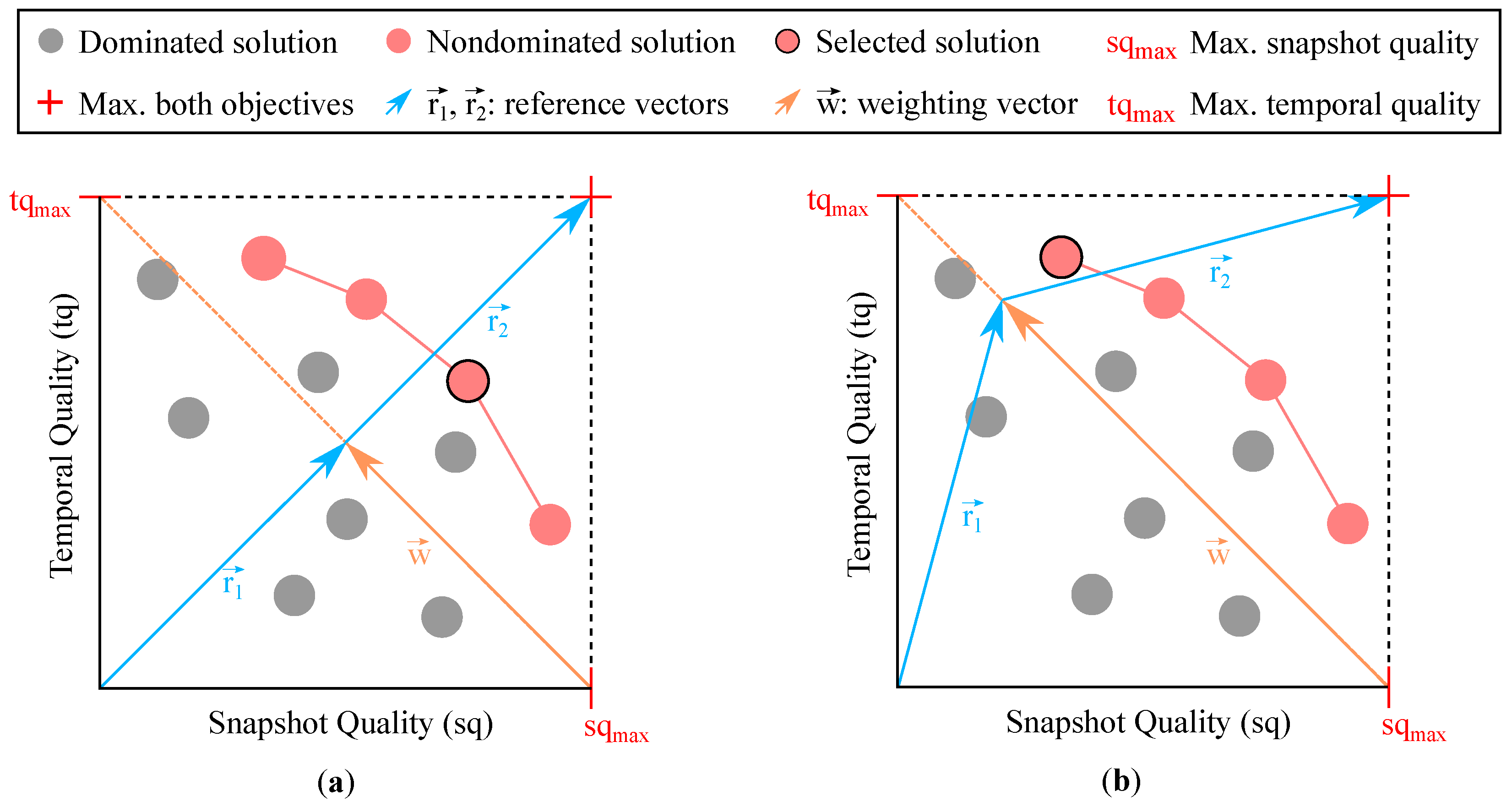
3.1. Weighting Procedure

Our weighting system is illustrated in Figure 1. Here, in both subfigures, the x-axis indicates values of snapshot quality, where $s{q}_{max}$ is the maximum possible value for the chosen metric. The y-axis denotes temporal quality values, with $t{q}_{max}$ representing the maximum. The grey circles are dominant solutions, and the pink circles form the Pareto front. The black outlined circle highlights the selected solution from the Pareto front. The segments are represented through two vectors, $\overrightarrow{r_1}$ and $\overrightarrow{r_2}$, which are further denoted as reference vectors (highlighted in blue). $\overrightarrow{w}$ is the weighting vector, which determines the position of the terminal point of $\overrightarrow{r_1}$ and the initial point of $\overrightarrow{r_2}$. The weight, $w\in [0,1]$, indicates the length of $\overrightarrow{w}$ relative to its maximum possible length.

Based on our construction, $w=0.5$ leads to a weighting vector of half of its maximum length, as shown in Figure 1a, where the reference vectors are collinear. In this case, both objectives have the same importance when selecting a solution from the Pareto front.

A weight of $w<0.5$ results in a lower weighting vector compared to $w=0.5$, shifting the terminal point of $\overrightarrow{r_1}$ and the initial point of $\overrightarrow{r_2}$ along the direction of $\overrightarrow{w}$ towards the position $(s{q}_{max},0)$, emphasising the importance of snapshot quality over temporal quality.

A weight $w>0.5$ leads to a larger weighting vector, shifting the terminal point of $\overrightarrow{r_1}$ and the initial point of $\overrightarrow{r_2}$ along the direction of $\overrightarrow{w}$ towards the position $(0,t{q}_{max})$. An example of this case with $w=0.8$ is shown in Figure 1b, whereby the new position of the reference vectors leads to the selection of another solution from the Pareto front compared to the selection from Figure 1a.

Lastly, $w=1$ results in $\overrightarrow{r_1}$ lying on the y-axis and $\overrightarrow{r_2}$ being parallel to the x-axis and vice versa for $w=0$. Thus, for $w=1$, the solution with the maximum temporal quality is selected, and for $w=0$, the solution with the maximum snapshot quality is chosen.

The mathematical formulation of our weighting procedure is presented, with all terms used, in

Table 1. Descriptions of terms used for the mathematical definition.

Term	Description
$s{q}_{max}$	Maximum snapshot quality
$t{q}_{max}$	Maximum temporal quality
$s{q}_t$	Snapshot quality of given solution at time t
$t{q}_t$	Temporal quality of given solution at time t
w	weight with $w\in [0,1]$

.

Since the initial and terminal points of the reference vectors are determined differently from each other, the corresponding equations for the distance calculation also differ from each other. The equation for the distance, $d_{r_1}$, of a Pareto optimal solution, $p=(s{q}_t,t{q}_t)$, with respect to the reference vector $\overrightarrow{r_1}$ is as follows:

$$d_{r_1}={\displaystyle \frac{\left|\left(\begin{array}{c}s{q}_t\\ t{q}_t\end{array}\right)\times \left(\begin{array}{c}s{q}_{max}-s{q}_{max}·w\\ t{q}_{max}·w\end{array}\right)\right|}{\left|\left(\begin{array}{c}s{q}_{max}-s{q}_{max}·w\\ t{q}_{max}·w\end{array}\right)\right|}}$$

(1)

In contrast, the distance, $d_{r_2}$, of the solution $p=(s{q}_t,t{q}_t)$ with respect to $\overrightarrow{r_2}$ is as follows:

$$d_{r_2}={\displaystyle \frac{\left|\left(\begin{array}{c}s{q}_t-s{q}_{max}+s{q}_{max}·w\\ t{q}_t-t{q}_{max}·w\end{array}\right)\times \left(\begin{array}{c}s{q}_{max}\\ t{q}_{max}\end{array}\right)\right|}{\left|\left(\begin{array}{c}s{q}_{max}\\ t{q}_{max}\end{array}\right)\right|}}$$

(2)

To decide which reference vector to use, the distance of a Pareto optimal solution, $p=(t{q}_t,s{q}_t)$, at time t should be calculated. We check whether a given solution lies over or under the vector $\overrightarrow{v}$ with the starting point at $(s{q}_{max},0)$ and the terminal point at $(0,t{q}_{max})$. The equation for this is defined as follows:

$$h(s{q}_t,t{q}_t)=s{q}_t·t{q}_{max}-s{q}_{max}·t{q}_{max}+t{q}_t·s{q}_{max}$$

(3)

If $h(s{q}_t,t{q}_t)>0$, then $\overrightarrow{r_2}$ should be used in the distance calculation. If $h(s{q}_t,t{q}_t)\le 0$, then $\overrightarrow{r_1}$ should be used, as shown in the following equation:

$$d=\left\{\begin{array}{cc}{d}_{r_2},\hfill & \mathrm{if}h(s{q}_t,t{q}_t)>0\hfill \\ d_{r_1},\hfill & \mathrm{otherwise}\hfill \end{array}\right.$$

(4)

Although Pareto fronts can have different lengths and shapes, a user should not have to consider them in order to set their preferred weight. To overcome this challenge, we assume we have an arbitrary continuous Pareto front, $P_c$. This allows us to partially determine the endpoints of $P_c$, as they lie on $s{q}_{max}$ and $t{q}_{max}$, enabling us to fulfil the following constraints for enhancing the user experience:

• Weights with $w\in \{0,1\}$ should match the endpoints of $P_c$;
• Every element from $P_c$ should be selectable by an appropriate weight (surjectivity);
• Two different weights should not map to the same element on $P_c$ (injectivity).

From the second and third constraints, it follows that the weighting system should be bijective. To clarify the third constraint in particular, let us assume a non-injective weighting system with only one reference vector, as shown in Figure 2. This vector has a fixed point at the minimum of both objectives and a weight indicating the angle between it and one of the axes. Suppose we have a continuous Pareto front, $P_c^{\prime }$, with endpoints $a=(0.8,1)$ and $z=(1,0.8)$. In this case, every weight with $w>=0.58$ would lead to the selection of a solution $a\in P_c^{\prime }$, as illustrated in Figure 2, and every $w<0.43$ would result in the selection of a solution $z\in P_c^{\prime }$. In contrast to our solution, such a weighting system implies decreasing sensibility with decreasing distance between the Pareto front and the maximum of both objectives, adding complexity and potentially reducing user-friendliness.

3.2. Transition-Based Temporal Quality Metric

Different clustering algorithms require different metrics for temporal quality based on their properties. Given the absence of established metrics for evaluating the temporal quality of density-based clusterings, in the following, we introduce a novel metric that is based on the movements of objects across different clusters over time. The foundation of this metric is the Jaccard coefficient, defined as follows for two sets A and B:

$$J(A,B)={\displaystyle \frac{|A\cap B|}{|A\cup B|}}$$

(5)

For the formulation of the metric, the concept of cluster transitions initially introduced by Korlakov et al. [4] is necessary. Given clusterings ${\widehat{C}}_{i,t-1}$ and ${\widehat{C}}_{j,t}$ at times t and $t-1$ with a set of time series D, the set of cluster transitions $T_t$ at time t is defined as follows:

$$\begin{array}{cc}{T}_t=& \left\{\right(C_{k,t-1},C_{m,t})|C_{k,t-1}\in {\widehat{C}}_{i,t-1}\wedge C_{m,t}\in {\widehat{C}}_{j,t}\wedge \hfill \\ & \exists s_{t-1},s_t\in S\in D:s_{t-1}\in C_{k,t-1}\wedge s_t\in C_{m,t}\}\end{array}$$

(6)

So, a single cluster transition is a tuple of two clusters $(C_{k,t-1},C_{m,t})$ of adjacent time points, with a time series S containing elements $s_{t-1}$ and $s_t$ lying in these clusters.

With Equations (5) and (6) in mind, our definition of the Jaccard-based temporal quality, $t{q}_t$, at time t is as follows:

$$t{q}_t={\displaystyle \frac{{\displaystyle \sum _{(C_{m,t}\in {\widehat{C}}_{i,t})}}{\displaystyle \sum _{(C_{n,t-1}\in {\widehat{C}}_{j,t-1})}}J(C_{m,t},C_{n,t-1})}{|T_t|}}$$

(7)

4. Experiments

For the evaluation of the proposed framework, several aspects need to be taken into account, including different datasets, clustering algorithms and parameters, frameworks for clustering over time and weightings for these frameworks. Since MOSCAT returns a set of clusterings, one for each time step, time is another component that has to be considered in the presentation of the results.

In order to provide a clear overview of the evaluation, we first present the datasets used. Next, we introduce the frameworks that we utilised for the comparison with the solutions presented in this work. Following that, details about the employed clustering algorithms and the associated framework metrics are provided. Next, the weight-setting process is explained. Finally, the results of the evaluation are presented and discussed.

4.1. Datasets and Frameworks for Comparison

We used two labelled datasets to evaluate the performance of our framework. The properties of both of them are shown in

Table 2. Properties of datasets used in experiments.

Dataset	No. Features	No. Time Series	No. Classes	Time Series Length
ERing	4	300	6	65
Motions	6	80	4	100

. The data for the first dataset, ERing, were gathered through a process of recording a variety of hand gestures [29]. This was conducted while the subject was wearing a prototype ring designed to generate an electric field. The second dataset, Motions, was taken from the website timeseriesclassification.com (https://www.timeseriesclassification.com/description.php?Dataset=BasicMotions, accessed on 6 January 2024). It consists of activity recordings of students, which were obtained with smart watches. These were the only datasets we could find online that were publicly accessible and met our requirements for the evaluation: multiple multivariate time series with labels and without missing values.

To evaluate the performance of our solution, we compared it to a baseline and Evolutionary Clustering [7]. The baseline involves static clustering per time point without considering the temporal context. The goal of Evolutionary Clustering is to maximise the following equation for the current point in time t: $s{q}_t-w·h{c}_t$. Here, snapshot quality $s{q}_t$ is the quality of a clustering at t, and $h{c}_t$ is the history cost, the quantified dissimilarity between the current clustering and the clustering at $t-1$.

4.2. Instantiations of Clustering Algorithms

Both frameworks rely on an underlying clustering algorithm. To showcase the versatility of our framework, we employ two different clustering algorithms, namely DBSCAN [30] and incremental K-Means for time series proposed by Chakrabarti et al. [7]. In the case of DBSCAN, the procedure for clustering over time is as follows:

• Cluster all time series at time t with all combinations of $ϵ\in \{p/q|q=10\wedge p\in ]0,10]\}$ and $\mathit{MinPts}\in [2,10]$.
• Let each framework select a clustering from the set of resulting clusterings.
• Move to the next time point, $t+1$.

The workflow of the incremental K-Means version for time series proposed by Chakrabarti et al. [7] is different. The authors state that each centroid at the current time t of their K-Means solution lies somewhere between the corresponding centroid at $t-1$ and the centroid resulting from static (without temporal context) k-Means clustering at time t. Centroid selection is determined by the weight of the Evolutionary Clustering. To ensure comparability between the frameworks, we also applied their version of incremental K-Means for time series. However, in our case, the selection process for the centroids is performed by MOSCAT. Further, we applied the Maximin method [31] in order to initialise the centroids at time $t=0$.

4.3. Framework Parameter Settings and Clustering Evaluation Metric

The selection of metrics for snapshot and temporal quality depends on the underlying clustering algorithm. For example, centroid-based metrics may not be the right choice for a clustering that could contain non-spherical cluster shapes. Therefore, with respect to DBSCAN, we use the silhouette coefficient [32] to measure the snapshot quality. The temporal quality is quantified by the Jaccard-based metric proposed in Section 3.2. For the measurement of the snapshot and temporal quality of incremental K-Means for clustering over time, we use the same metrics as suggested by Chakrabarti et al. [7].

In general, any strategy for selecting a solution from a Pareto front can be used in our framework to determine the weight. However, for simplicity, we applied TOPSIS (Technique of Order Preference Similarity to the Ideal Solution) [19], with the objectives for the resulting Pareto fronts from both datasets and clustering algorithms being equalliy important. TOPSIS is a technique used to order the solutions from the Pareto front based on their similarity to the ideal and anti-ideal solutions.

We selected the weight for our framework according to the solution with the highest score. In the case of Evolutionary Clustering, we set the weight w to $w=0.1$, as suggested by the authors of [7]. In order to compare the quality of the clusterings of both frameworks and the baseline, we use a metric called purity [33]. It is an external evaluation criterion of cluster quality and indicates the average number of objects in the majority class presented in each cluster.

4.4. Results

In our evaluation, we assume that the user’s task involves clustering unfamiliar data. Consequently, the user’s access is restricted to the following information: the dataset itself, the clustering results and the snapshot and temporal qualities. Additionally, they have the ability to assign the weight of the temporal context to both clustering frameworks. Notably, the user lacks access to the labels associated with the datasets.

To provide a summarised presentation of the results, we show the mean and standard deviation of the purity across the clusterings over time for both datasets. The framework-specific weight is set once at the beginning of the over-time clustering process. It is important to distinguish between the underlying clustering algorithms and their respective evaluations. For DBSCAN, both clustering frameworks choose from a set of clusterings generated through different combinations of $ϵ$ and MinPts. In contrast, for incremental K-Means, both frameworks select from a set of clusterings created separately for each $k\in [2,10]$ after each centroid recalculation.

Table 3. Average purity over time for both frameworks with DBSCAN as the underlying clustering algorithm.

Dataset	Baseline	Evol. Clustering	MOSCAT
ERing	0.191 ± 0.058	0.178 ± 0.005	0.180 ± 0.004
Motions	0.288 ± 0.057	0.284 ± 0.049	0.477 ± 0.057

illustrates the purity achieved with DBSCAN as the underlying clustering algorithm, the silhouette coefficient as a snapshot quality metric, and the transition-based metric proposed in Section 3.2 for temporal quality. Evolutionary Clustering performs worse than MOSCAT and the baseline. In contrast, MOSCAT exhibits the highest purity value for the Motions dataset. The baseline shows the highest purity for the ERing dataset, indicating that prioritising snapshot and temporal quality does not always maximise the purity.

The clustering performance with incremental K-Means as the underlying clustering algorithm is illustrated in

Table 4. Average purity over time with K-Means as the underlying clustering algorithm.

		Purity			Weight
Dataset	k	Baseline	Evol. Clustering	MOSCAT	MOSCAT
Motions	2	0.371 ± 0.016	0.280 ± 0.016	0.280 ± 0.016	0.8
	3	0.388 ± 0.048	0.421 ± 0.044	0.397 ± 0.037	0.9
	4	0.450 ± 0.046	0.485 ± 0.039	0.469 ± 0.042	0.8
	5	0.451 ± 0.045	0.479 ± 0.038	0.465 ± 0.051	0.8
	6	0.476 ± 0.035	0.497 ± 0.030	0.504 ± 0.047	0.8
	7	0.459 ± 0.048	0.499 ± 0.026	0.547 ± 0.047	0.8
	8	0.485 ± 0.042	0.503 ± 0.026	0.507 ± 0.043	0.7
	9	0.484 ± 0.040	0.500 ± 0.024	0.510 ± 0.048	0.7
	10	0.461 ± 0.047	0.501 ± 0.026	0.510 ± 0.059	0.7
ERing	2	0.325 ± 0.013	0.324 ± 0.013	0.325 ± 0.013	0.0
	3	0.448 ± 0.039	0.445 ± 0.045	0.448 ± 0.039	0.0
	4	0.535 ± 0.063	0.530 ± 0.069	0.536 ± 0.061	0.8
	5	0.524 ± 0.069	0.537 ± 0.069	0.526 ± 0.066	0.8
	6	0.569 ± 0.071	0.573 ± 0.077	0.567 ± 0.074	0.8
	7	0.586 ± 0.086	0.587 ± 0.088	0.589 ± 0.085	0.8
	8	0.598 ± 0.076	0.582 ± 0.077	0.600 ± 0.079	0.7
	9	0.602 ± 0.078	0.592 ± 0.079	0.604 ± 0.082	0.7
	10	0.611 ± 0.074	0.602 ± 0.076	0.612 ± 0.078	0.8

. While Evolutionary Clustering outperforms our framework in only 5 of 18 cases, the results for the ERing dataset reveal that, for four different values of k, Evolutionary Clustering is surpassed by the baseline. In contrast, the baseline manages to outperform MOSCAT only once in the same dataset. For the Motions dataset, the baseline outperforms both frameworks only once for $k=2$. However, in most cases, our solution yields superior results in terms of purity.

Despite drawing comparisons between the frameworks, the consideration of the weight of MOSCAT highlights that our framework places significant importance on the temporal context of both datasets. This is particularly evident for the Motions dataset, where our framework leads to a significant increase in purity compared to the baseline. Assuming that $w=1$ leads to a maximal temporal context, i.e., one in which the centroid positions do not change over time, the weights for several values of k show that the centroids of both datasets undergo relatively small shifts over time. However, in the case of the ERing dataset and $k\in [2,3]$, the opposite is true. In this scenario, the centroid positions undergo significant changes over time.

In general, our framework surpasses Evolutionary Clustering in three key aspects. First, the weight of Evolutionary Clustering can lead to unnecessary fluctuations in $sq$ and $tq$, potentially resulting in poorer clusterings across time. Consider, for instance, having a weight w with $w=0.5$ and four tuples of shape $(sq,tq)$ (each tuple corresponds to a clustering) with values $(0.8,0.3)$ and $(0.6,0.4)$ at time t and $(0.4,0.6)$ and $(0.3,0.9)$ at time $t+1$. In this scenario, Evolutionary Clustering would select the clusterings with $(0.8,0.3)$ at time $t=1$ and $(0.3,0.9)$ at time $t=2$. However, the fluctuations in the qualities of these clusterings are higher compared to the other two clusterings with $(0.6,0.4)$ and $(0.4,0.6)$, which our framework would select for the same weight. Secondly, while our approach enables the selection of any solution on the Pareto front, there are solutions that cannot be chosen by Evolutionary Clustering. An example of this involves clusterings with the following values for $sq$ and $tq$: $(0.9,0.1),(0.5,0.5)$, and $(0.1,0.9)$. Here, regardless of the weight w, the solution with $(0.5,0.5)$ will not be selected, although it lies on the Pareto front along with the other solutions. Lastly, in the case of Evolutionary Clustering, the number of distinct solutions with the same overall quality score for a fixed weight can theoretically be infinitely large, which may have a negative impact on the clustering result and usability in general (e.g., $(0.76,0.9),(0.8,0.5),(0.81,0.4),(0.84,0.1)$ for $w=0.1$). In contrast, the design of our approach only allows two solutions to be selected simultaneously.

5. Conclusions and Future Work

In this work, we introduced MOSCAT, a new framework designed for clustering multiple multivariate time series over time. Our approach extracts the Pareto front considering the objectives for snapshot and temporal quality. The corresponding weighting procedure enables the determination of the weight through a number of already existing solutions, providing users with the option for precise weight calibration based on their preferences. Furthermore, we discussed metrics for snapshot and temporal quality, proposing a temporal quality metric specifically designed for clustering algorithms that are not centroid-based.

In our experiments, we compared the performance of MOSCAT with Evolutionary Clustering and a baseline using DBSCAN and incremental K-Means as underlying clustering algorithms. The results showed that our framework outperforms both Evolutionary Clustering and the baseline in the majority of cases. Furthermore, the results demonstrated the informative value of MOSCAT’s weights.

Although our framework shows convincing clustering results, there are a few aspects that should be investigated further. In our evaluation, we applied TOPSIS for the weight determination of our framework. Since there are many other strategies for selecting solutions, it is crucial to analyse what influence these have on the clustering result. Depending on this, several strategies could be combined to reach a majority decision, which could reduce the uncertainties in the individual strategies. Additionally, our weighting procedure can be used for tracking the decisions of solution selection strategies within the over-time clustering process. This enables comparisons between different datasets with regard to their temporal dependencies, which we intend to analyse in future work. Further, the tracking of the solution selection process could reveal hidden patterns in time series or be used to detect anomalies between adjacent points in time. Finally, a more thorough exploration of the relationship between snapshot and temporal quality could help to develop a solution selection strategy that explicitly takes these objectives into account. However, all the topics mentioned necessitate more labelled datasets containing multiple multivariate time series. For this purpose, we are currently collecting additional datasets from different domains.

References

1. James, N.; Menzies, M. Cluster-based dual evolution for multivariate time series: Analyzing COVID-19. Chaos Interdiscip. J. Nonlinear Sci. 2020, 30, 61108. [Google Scholar] [CrossRef]
2. Simmhan, Y.; Noor, M.U. Scalable prediction of energy consumption using incremental time series clustering. In Proceedings of the 2013 IEEE International Conference on Big Data, Silicon Valley, CA, USA, 6–9 October 2013; IEEE: Piscataway, NJ, USA, 2013; pp. 29–36. [Google Scholar]
3. Gružauskas, V.; Čalnerytė, D.; Fyleris, T.; Kriščiūnas, A. Application of multivariate time series cluster analysis to regional socioeconomic indicators of municipalities. Real Estate Manag. Valuat. 2021, 29, 39–51. [Google Scholar] [CrossRef]
4. Korlakov, S.; Klassen, G.; Bravidor, M.; Conrad, S. Alone We Can Do So Little; Together We Cannot Be Detected. Eng. Proc. 2022, 18, 3. [Google Scholar] [CrossRef]
5. Abdallah, I.; Duthé, G.; Barber, S.; Chatzi, E. Identifying evolving leading edge erosion by tracking clusters of lift coefficients. Proc. J. Phys. Conf. Ser. 2022, 2265, 32089. [Google Scholar] [CrossRef]
6. Klassen, G.; Tatusch, M.; Huo, W.; Conrad, S. Evaluating machine learning algorithms in predicting financial restatements. In Proceedings of the 2020 The 4th International Conference on Business and Information Management, Rome, Italy, 3–5 August 2020; ACM: New York, NY, USA, 2020; pp. 95–100. [Google Scholar]
7. Chakrabarti, D.; Kumar, R.; Tomkins, A. Evolutionary clustering. In Proceedings of the 12th ACM SIGKDD International Conference on Knowledge Discovery and Data Mining, Philadelphia, PA, USA, 20–23 August 2006; ACM: New York, NY, USA, 2006. [Google Scholar]
8. Chi, Y.; Song, X.; Zhou, D.; Hino, K.; Tseng, B.L. On evolutionary spectral clustering. ACM Trans. Knowl. Discov. Data (TKDD) 2009, 3, 1–30. [Google Scholar] [CrossRef]
9. Zhang, Y.; Liu, H.; Deng, B. Evolutionary clustering with DBSCAN. In Proceedings of the 2013 Ninth International Conference on Natural Computation (ICNC), Shenyang, China, 23–25 July 2013; IEEE: Piscataway, NJ, USA, 2013. [Google Scholar]
10. Li, T.; Chen, L.; Jensen, C.S.; Pedersen, T.B.; Gao, Y.; Hu, J. Evolutionary clustering of moving objects. In Proceedings of the 2022 IEEE 38th International Conference on Data Engineering (ICDE), Kuala Lumpur, Malaysia, 9–12 May 2022; IEEE: Piscataway, NJ, USA, 2022. [Google Scholar]
11. Shankar, R.; Kiran, G.; Pudi, V. Evolutionary clustering using frequent itemsets. In Proceedings of the First International Workshop on Novel Data Stream Pattern Mining Techniques, Washington, DC, USA, 25 July 2010; ACM: New York, NY, USA, 2010. [Google Scholar]
12. Ma, X.; Zhang, B.; Ma, C.; Ma, Z. Co-regularized nonnegative matrix factorization for evolving community detection in dynamic networks. Inf. Sci. 2020, 528, 265–279. [Google Scholar] [CrossRef]
13. Chi, Y.; Song, X.; Zhou, D.; Hino, K.; Tseng, B.L. Evolutionary spectral clustering by incorporating temporal smoothness. In Proceedings of the 13th ACM SIGKDD International Conference on Knowledge Discovery and Data Mining, San Jose, CA, USA, 12–15 August 2007; ACM: New York, NY, USA, 2007. [Google Scholar]
14. Putri, G.H.; Read, M.N.; Koprinska, I.; Singh, D.; Röhm, U.; Ashhurst, T.M.; King, N.J. ChronoClust: Density-based clustering and cluster tracking in high-dimensional time-series data. Knowl.-Based Syst. 2019, 174, 9–26. [Google Scholar] [CrossRef]
15. Zhang, J.; Song, Y.; Chen, G.; Zhang, C. On-line evolutionary exponential family mixture. In Proceedings of the Twenty-First International Joint Conference on Artificial Intelligence, Pasadena, CA, USA, 11–17 July 2009; IJCAI: San Francisco, CA, USA, 2009. [Google Scholar]
16. Xu, K.S.; Kliger, M.; Hero III, A.O. Adaptive evolutionary clustering. Data Min. Knowl. Discov. 2014, 28, 304–336. [Google Scholar] [CrossRef]
17. Klassen, G.; Tatusch, M.; Conrad, S. Cluster-based stability evaluation in time series data sets. Appl. Intell. 2023, 53, 16606–16629. [Google Scholar] [CrossRef] [PubMed]
18. Srinivasan, V.; Shocker, A.D. Linear programming techniques for multidimensional analysis of preferences. Psychometrika 1973, 38, 337–369. [Google Scholar] [CrossRef]
19. Hwang, C.; Yoon, K. Multiple Attribute Decision Making, Methods and Applications; Springer: Berlin/Heidelberg, Germany, 1981. [Google Scholar]
20. Deb, K.; Pratap, A.; Agarwal, S.; Meyarivan, T. A fast and elitist multiobjective genetic algorithm: NSGA-II. IEEE Trans. Evol. Comput. 2002, 6, 182–197. [Google Scholar] [CrossRef]
21. Martinez-Morales, J.D.; Pineda-Rico, U.; Stevens-Navarro, E. Performance comparison between MADM algorithms for vertical handoff in 4G networks. In Proceedings of the 2010 7th International Conference on Electrical Engineering Computing Science and Automatic Control, Tuxtla Gutierrez, Mexico, 8–10 September 2010; IEEE: Piscataway, NJ, USA, 2010. [Google Scholar]
22. Márquez, D.G.; Otero, A.; Félix, P.; García, C.A. A novel and simple strategy for evolving prototype based clustering. Pattern Recognit. 2018, 82, 16–30. [Google Scholar] [CrossRef]
23. Lin, Y.R.; Chi, Y.; Zhu, S.; Sundaram, H.; Tseng, B.L. Analyzing communities and their evolutions in dynamic social networks. ACM Trans. Knowl. Discov. Data (TKDD) 2009, 3, 1–31. [Google Scholar] [CrossRef]
24. Mucha, P.J.; Richardson, T.; Macon, K.; Porter, M.A.; Onnela, J.P. Community structure in time-dependent, multiscale, and multiplex networks. Science 2010, 328, 876–878. [Google Scholar] [CrossRef] [PubMed]
25. Du, N.; Jia, X.; Gao, J.; Gopalakrishnan, V.; Zhang, A. Tracking temporal community strength in dynamic networks. IEEE Trans. Knowl. Data Eng. 2015, 27, 3125–3137. [Google Scholar] [CrossRef]
26. Folino, F.; Pizzuti, C. An evolutionary multiobjective approach for community discovery in dynamic networks. IEEE Trans. Knowl. Data Eng. 2013, 26, 1838–1852. [Google Scholar] [CrossRef]
27. Yin, Y.; Zhao, Y.; Li, H.; Dong, X. Multi-objective evolutionary clustering for large-scale dynamic community detection. Inf. Sci. 2021, 549, 269–287. [Google Scholar] [CrossRef]
28. Li, W.; Zhou, X.; Yang, C.; Fan, Y.; Wang, Z.; Liu, Y. Multi-objective optimization algorithm based on characteristics fusion of dynamic social networks for community discovery. Inf. Fusion 2022, 79, 110–123. [Google Scholar] [CrossRef]
29. Wilhelm, M.; Krakowczyk, D.; Trollmann, F.; Albayrak, S. eRing: Multiple finger gesture recognition with one ring using an electric field. In Proceedings of the 2nd international Workshop on Sensor-Based Activity Recognition and Interaction, Rostock, Germany, 25–26 June 2015; ACM: New York, NY, USA, 2015. [Google Scholar]
30. Ester, M.; Kriegel, H.P.; Sander, J.; Xu, X. A density-based algorithm for discovering clusters in large spatial databases with noise. In Proceedings of the KDD, Portland, OR, USA, 2–4 August 1996; ACM: New York, NY, USA, 1996. [Google Scholar]
31. Gonzalez, T.F. Clustering to minimize the maximum intercluster distance. Theor. Comput. Sci. 1985, 38, 293–306. [Google Scholar] [CrossRef]
32. Rousseeuw, P.J. Silhouettes: A graphical aid to the interpretation and validation of cluster analysis. J. Comput. Appl. Math. 1987, 20, 53–65. [Google Scholar] [CrossRef]
33. Manning, C.D. An Introduction to Information Retrieval; Cambridge University Press: Cambridge, UK, 2009. [Google Scholar]
Figure 1. Selection process from an exemplary Pareto front. (a) Selection using a weight of 0.5 for temporal quality. (b) Selection using a weight of 0.8 for temporal quality.
Engproc 68 00048 g001
Figure 2. Example of a simple selection process from a Pareto front.
Engproc 68 00048 g002