
A Simple Computational Approach to Predict Long-Term Hourly Electric Consumption †


Abstract
1. Introduction
1.1. Related Work
1.2. Quick Summary
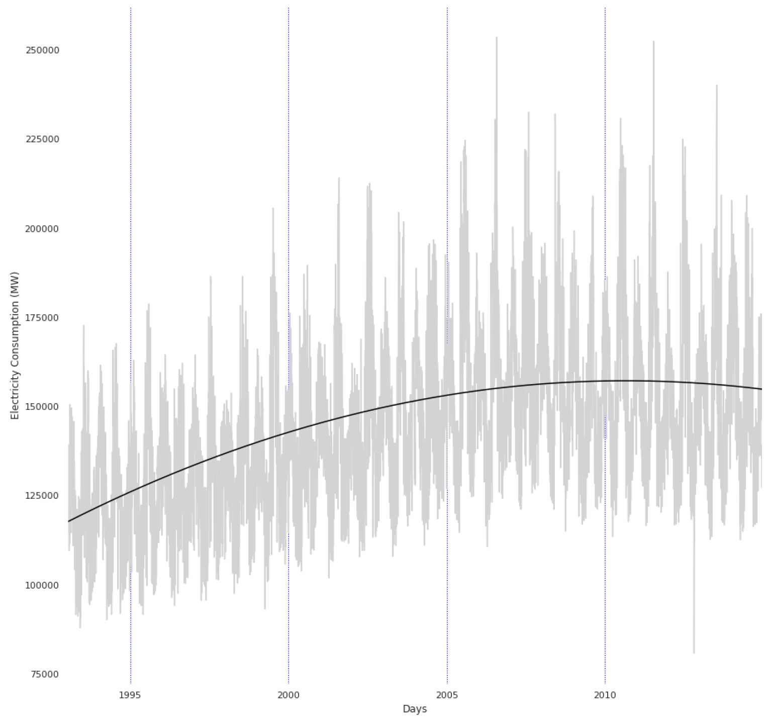
- Remove the major trend reflecting changes in the annual consumption. We do this by using a simple linear autoregression (we also tried a second-degree order linear auto-regression for some of the datasets). Note that after the trend is removed, it is still possible that the detrended time series is seasonal, and hence, non-stationary.
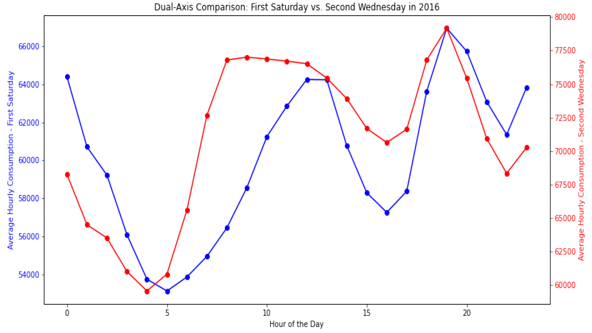
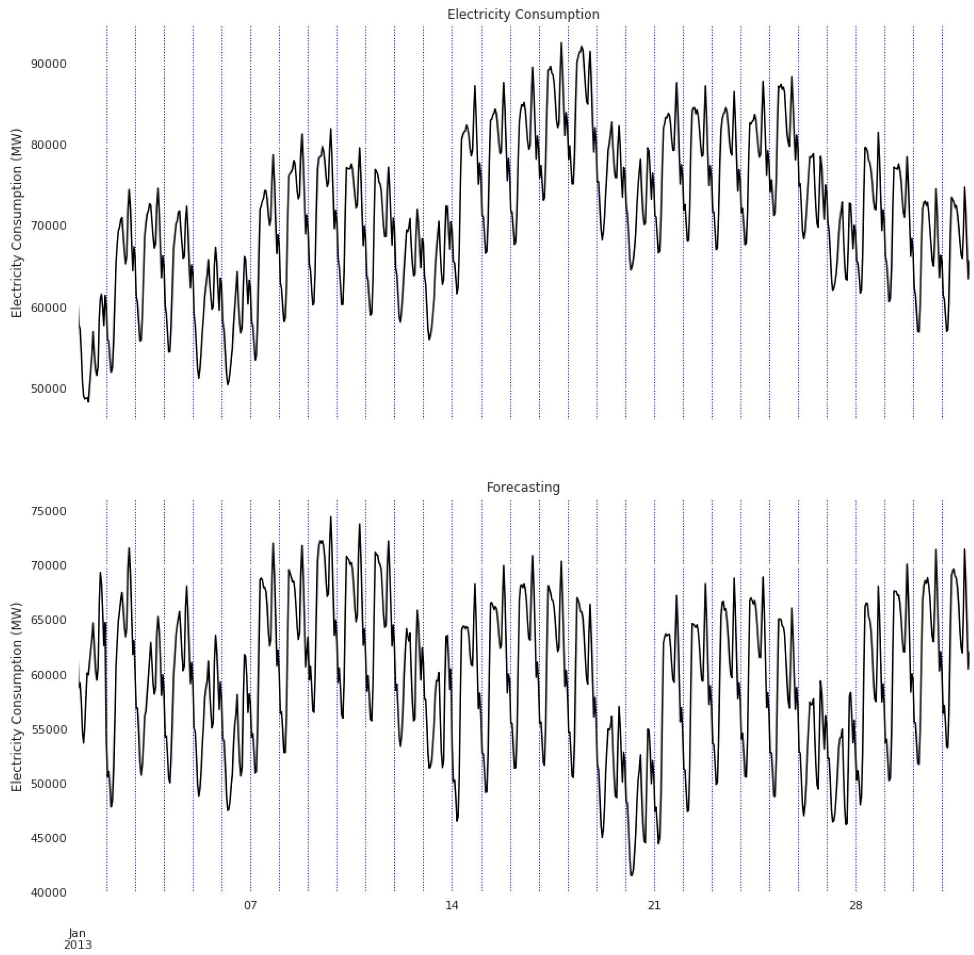
- We predict daily consumption for each day by looking at the appropriate average of the power consumption for “similar” days in the past.
2. Mathematical Notation and Preliminaries
2.1. Detrending
2.2. Mean Absolute Percentage Error
2.3. Confidence Interval
3. Development
3.1. Datasets
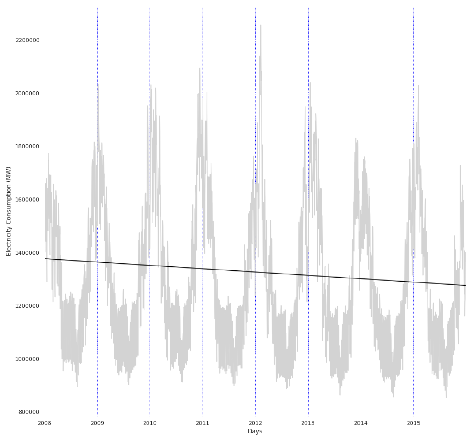
- The French Réseau de Transport d’Électricité (RTE) company, in charge of the French power distribution network, published its dataset of the overall half-hour consumption across all France from 2008 to 2018 [17].
- The same French RTE company published its dataset of the overall production of electricity produced by renewable resources in France (except Corsica) from 2012 to 2020.
- The American Independent System Operators (ISO) company, operating New England’s grid and in charge of power system planning, used to publish a dataset of hourly consumption in New England from 2004 to 2015.
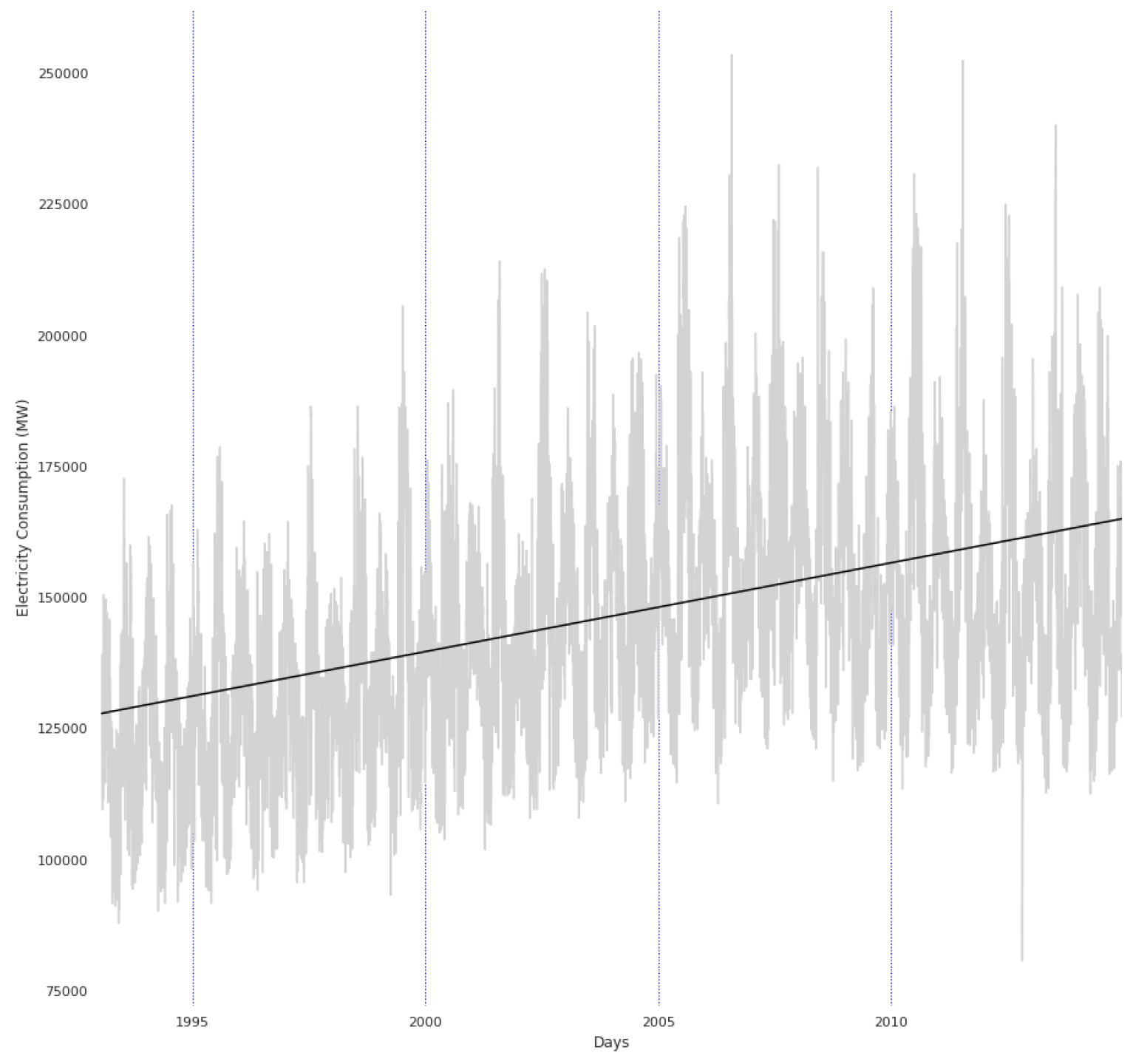
- The American Pennsylvania-New Jersey-Maryland Interconnection (PJM) organization [11] coordinates the movement of wholesale electricity in all parts of 13 US states. The organization published datasets of metered data aggregated from the zones’ respective electric distribution companies. We can find the datasets of hourly zone loads from as early as 1993, depending on the zones.
3.2. Pre-Processing
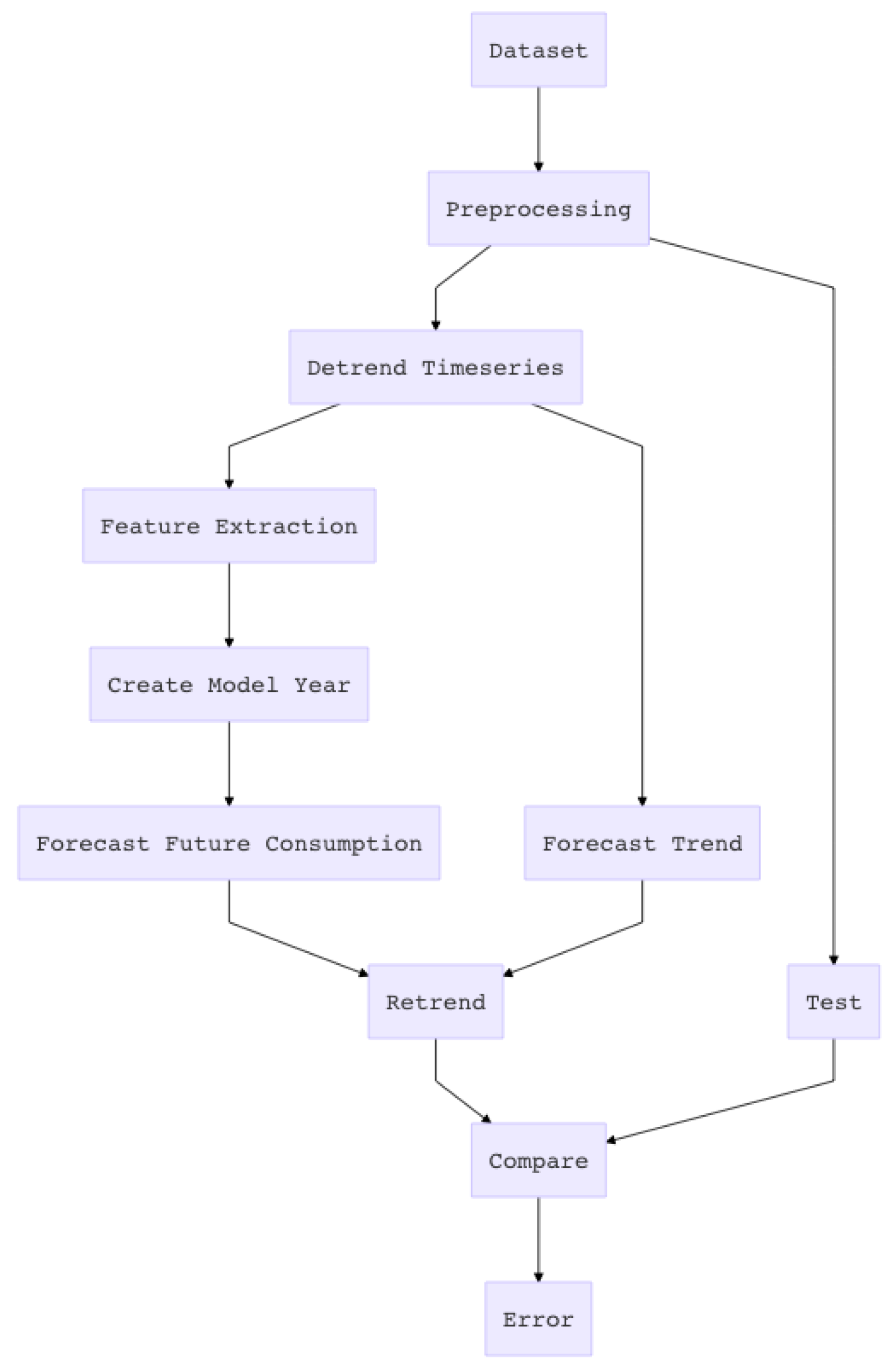
3.3. Schema of the Pipeline
3.4. Detrending Explanation
3.5. Model Year Explanation
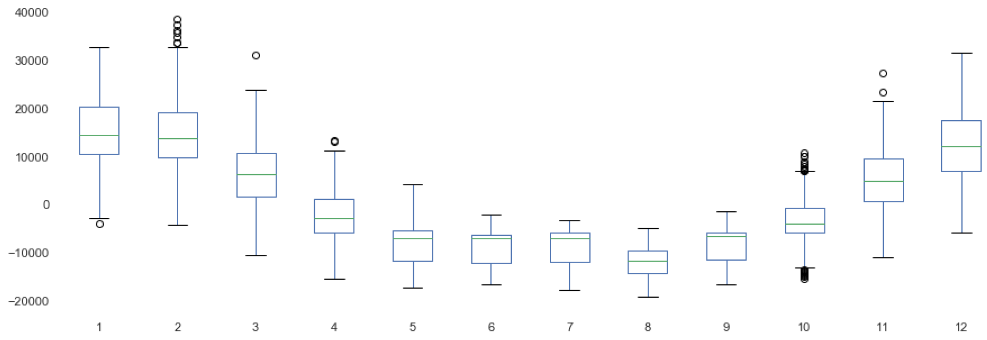
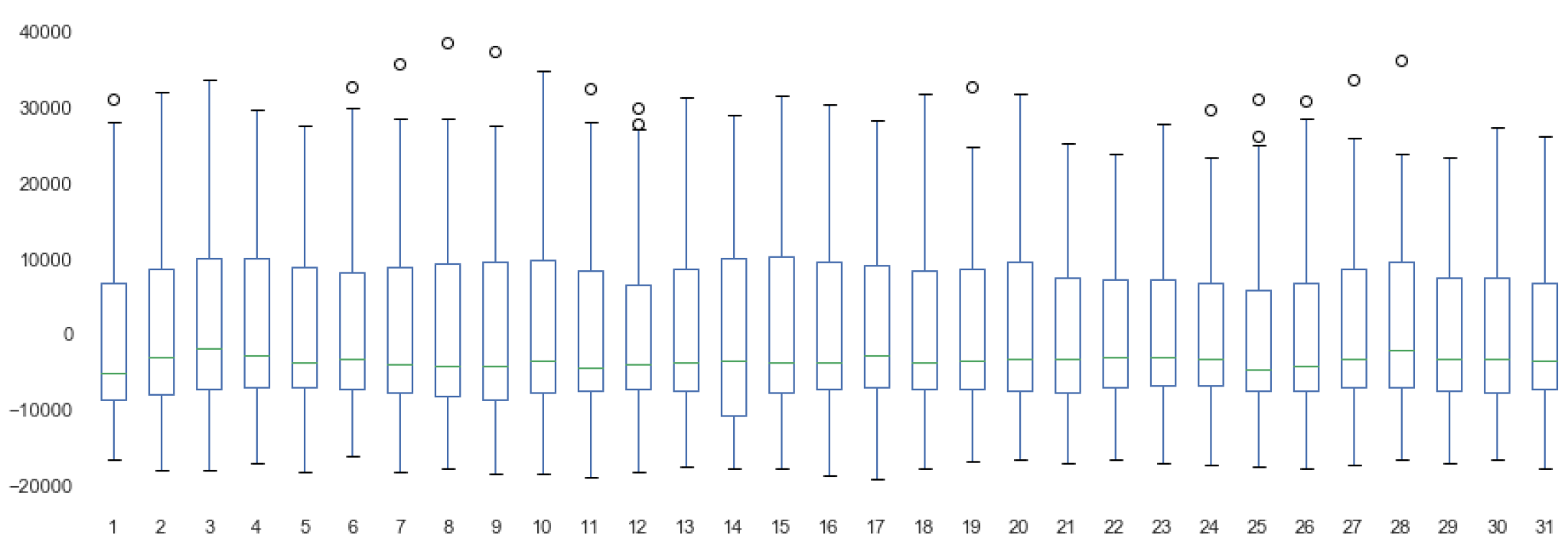
3.5.1. Data Analysis
3.5.2. Building the Model
3.5.3. Formula
4. Results
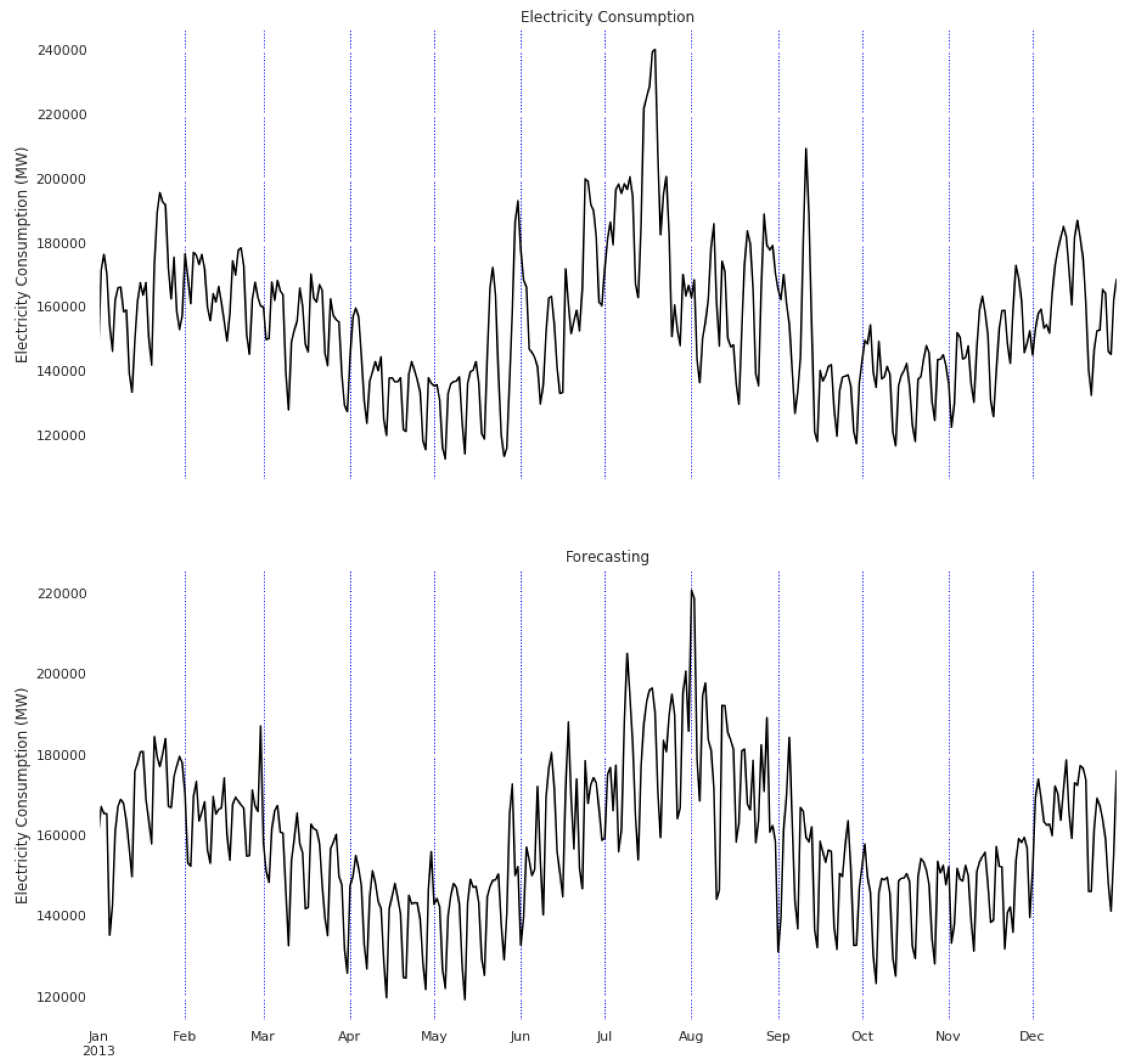
4.1. RTE Dataset
4.2. ISO Dataset
4.3. PJM Dataset
Improving the Detrending
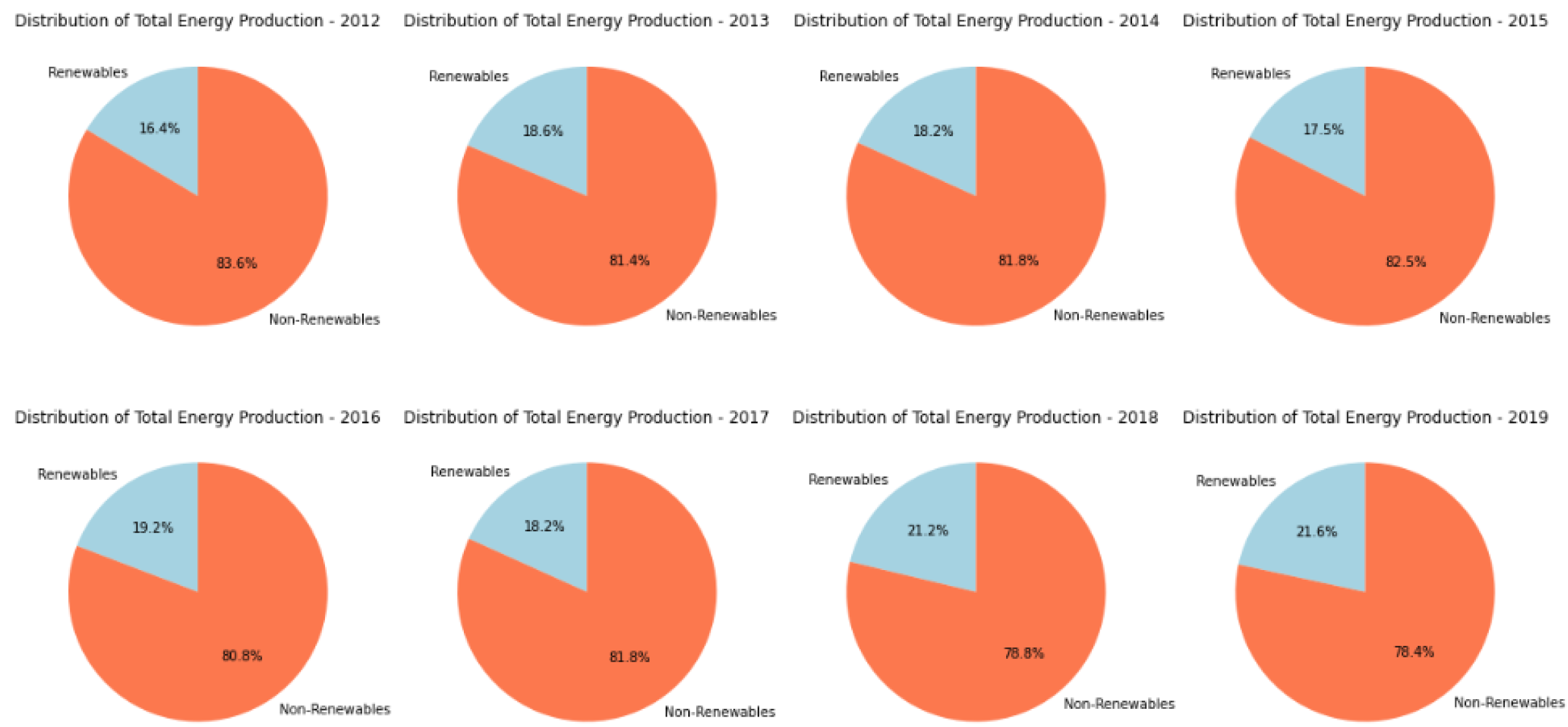
5. Renewable Energy Sources
6. Conclusions
Author Contributions
Funding
Institutional Review Board Statement
Informed Consent Statement
Data Availability Statement
Acknowledgments
Conflicts of Interest
References
- Hernandez, L.; Baladron, C.; Aguiar, J.M.; Calavia, L.; Carro, B.; Sanchez-Esguevillas, A.; Cook, D.J.; Chinarro, D.; Gomez, J. A Study of the Relationship between Weather Variables and Electric Power Demand inside a Smart Grid/Smart World Framework. Sensors 2012, 12, 11571–11591. [Google Scholar] [CrossRef]
- Jones, R.V.; Fuertes, A.; Lomas, K.J. The socio-economic, dwelling and appliance related factors affecting electricity consumption in domestic buildings. Renew. Sustain. Energy Rev. 2015, 43, 901–917. [Google Scholar] [CrossRef]
- Sanquist, T.F.; Orr, H.; Shui, B.; Bittner, A.C. Lifestyle factors in US residential electricity consumption. Energy Policy 2012, 42, 354–364. [Google Scholar] [CrossRef]
- Agrawal, R.K.; Muchahary, F.; Tripathi, M.M. Long term load forecasting with hourly predictions based on long-short-term-memory networks. In Proceedings of the 2018 IEEE Texas Power and Energy Conference (TPEC), College Station, TX, USA, 8–9 February 2018; pp. 1–6. [Google Scholar] [CrossRef]
- Boroojeni, K.G.; Amini, M.H.; Bahrami, S.; Iyengar, S.; Sarwat, A.I.; Karabasoglu, O. A novel multi-time-scale modeling for electric power demand forecasting: From short-term to medium-term horizon. Electr. Power Syst. Res. 2017, 142, 58–73. [Google Scholar] [CrossRef]
- Bouktif, S.; Fiaz, A.; Ouni, A.; Serhani, M. Optimal Deep Learning LSTM Model for Electric Load Forecasting using Feature Selection and Genetic Algorithm: Comparison with Machine Learning Approaches. Energies 2018, 11, 1636. [Google Scholar] [CrossRef]
- Esteves, G.R.; Bastos, B.Q.; Cyrino, F.L.; Calili, R.F.; Souza, R.C. Long term electricity forecast: A systematic review. Procedia Comput. Sci. 2015, 55, 549–558. [Google Scholar] [CrossRef]
- Daneshi, H.; Shahidehpour, M.; Choobbari, A.L. Long-term load forecasting in electricity market. In Proceedings of the 2008 IEEE International Conference on Electro/Information Technology, Ames, IA, USA, 18–20 May 2008; IEEE: Piscataway, NJ, USA, 2008; pp. 395–400. [Google Scholar]
- Goude, Y.; Nedellec, R.; Kong, N. Local Short and Middle Term Electricity Load Forecasting with Semi-Parametric Additive Models. IEEE Trans. Smart Grid 2014, 5, 440–446. [Google Scholar] [CrossRef]
- Khuntia, S.; Rueda, J.; van der Meijden, M. Long-Term Electricity Load Forecasting Considering Volatility Using Multiplicative Error Model. Energies 2018, 11, 3308. [Google Scholar] [CrossRef]
- PJM. Systems Operations. Available online: https://www.pjm.com/markets-and-operations/ops-analysis/ (accessed on 4 March 2024).
- Safdarian, A.; Fotuhi-Firuzabad, M.; Lehtonen, M.; Aghazadeh, M.; Ozdemir, A. A new approach for long-term electricity load forecasting. In Proceedings of the 2013 8th International Conference on Electrical and Electronics Engineering (ELECO), Bursa, Turkey, 28–30 November 2013; IEEE: Piscataway, NJ, USA, 2013; pp. 122–126. [Google Scholar]
- ISO New England. Pricing Reports. Available online: https://www.iso-ne.com/isoexpress/web/reports/ (accessed on 4 March 2024).
- Hong, T.; Xie, J.; Black, J. Global energy forecasting competition 2017: Hierarchical probabilistic load forecasting. Int. J. Forecast. 2019, 35, 1389–1399. [Google Scholar] [CrossRef]
- Ziel, F. Quantile regression for the qualifying match of GEFCom2017 probabilistic load forecasting. Int. J. Forecast. 2018, 35, 1400–1408. [Google Scholar] [CrossRef]
- Smyl, S.; Hua, N.G. Machine learning methods for GEFCom2017 probabilistic load forecasting. Int. J. Forecast. 2019, 35, 1424–1431. [Google Scholar] [CrossRef]
- France, R. Consumption API. Available online: https://data.rte-france.com/catalog/-/api/consumption/Consumption/v1.2 (accessed on 4 March 2024).
- Meunier, E.; Moreau, P.; Sharma, T. Our Open Sourced Code on GitHub. Available online: https://github.com/tanvisharmaaa/France_Electricity_Visualisations (accessed on 4 March 2024).


| Year | Our MAPE | Our Confidence Interval |
|---|---|---|
| 2012 | 6.79 | 10.07 |
| 2013 | 5.75 | 8.95 |
| 2014 | 5.1 | 8.09 |
| 2015 | 5.38 | 8.11 |
| 2016 | 5.51 | 7.77 |
| 2017 | 5.88 | 8.47 |
| 2018 | 6.23 | 12.89 |
| Overall | 7.07 | 4.71 |
| Year | Our MAPE | Our Confidence Interval | [4] MAPE | [4] Confidence Interval |
|---|---|---|---|---|
| 2010 | 5.69 | 8.31 | ||
| 2011 | 5.62 | 8.02 | 5.6 | 4.8 |
| 2012 | 6.18 | 8.67 | 7.5 | 1.61 |
| 2013 | 6.11 | 8.29 | 6.6 | 6.35 |
| 2014 | 6.5 | 7.85 | 6.6 | 5.19 |
| 2015 | 7.21 | 11.44 | 6.17 | 6.38 |
| Overall | 6.34 | 4.99 | 6.54 | 2.25 |
| Year | Our MAPE | Our Confidence Interval |
|---|---|---|
| 2010 | 9.73 | 9.33 |
| 2011 | 11.07 | 12.27 |
| 2012 | 11.68 | 12.31 |
| 2013 | 10.96 | 10.59 |
| 2014 | 10.38 | 14.11 |
| Overall | 12.67 | 7.88 |
| Year | Our MAPE | Our Confidence Interval |
|---|---|---|
| 2010 | 8.28 | 8.72 |
| 2011 | 9.35 | 11.39 |
| 2012 | 10.00 | 11.45 |
| 2013 | 9.38 | 9.49 |
| 2014 | 9.05 | 9.49 |
| Overall | 10.04 | 6.80 |
Disclaimer/Publisher’s Note: The statements, opinions and data contained in all publications are solely those of the individual author(s) and contributor(s) and not of MDPI and/or the editor(s). MDPI and/or the editor(s) disclaim responsibility for any injury to people or property resulting from any ideas, methods, instructions or products referred to in the content. |
© 2024 by the authors. Licensee MDPI, Basel, Switzerland. This article is an open access article distributed under the terms and conditions of the Creative Commons Attribution (CC BY) license (https://creativecommons.org/licenses/by/4.0/).
Share and Cite
Pinsky, E.; Meunier, E.; Moreau, P.; Sharma, T. A Simple Computational Approach to Predict Long-Term Hourly Electric Consumption. Eng. Proc. 2024, 68, 59. https://doi.org/10.3390/engproc2024068059
Pinsky E, Meunier E, Moreau P, Sharma T. A Simple Computational Approach to Predict Long-Term Hourly Electric Consumption. Engineering Proceedings. 2024; 68(1):59. https://doi.org/10.3390/engproc2024068059
Chicago/Turabian StylePinsky, Eugene, Etienne Meunier, Pierre Moreau, and Tanvi Sharma. 2024. "A Simple Computational Approach to Predict Long-Term Hourly Electric Consumption" Engineering Proceedings 68, no. 1: 59. https://doi.org/10.3390/engproc2024068059
APA StylePinsky, E., Meunier, E., Moreau, P., & Sharma, T. (2024). A Simple Computational Approach to Predict Long-Term Hourly Electric Consumption. Engineering Proceedings, 68(1), 59. https://doi.org/10.3390/engproc2024068059