Parameter Estimation in Water Distribution Networks Using an Error-in-Variables Approach ^†

Abstract

A well-calibrated model of a water distribution network is necessary for monitoring, control, and operation. In this work, we address the problem of parameter estimation in water distribution networks (WDNs). Typical parameters to be estimated include the coefficients used to model major (pipes) and minor (joints, etc.) losses due to friction. The problem of parameter estimation is a nonlinear regression problem and is solved using the error-in-variables approach. The method is illustrated using data from an experimental facility.

1. Introduction

A well-calibrated model of a water distribution network is necessary for monitoring, control, and operation. In this work, we address the problem of parameter estimation in water distribution networks (WDNs). Typical parameters to be estimated include the coefficients used to model major (pipes) and minor (joints, etc.) losses due to friction. The head loss in pipes is nonlinearly related to the flow through them (according to the Hazen–Williams equation). The minor losses and the head loss in valves are also related to the flow nonlinearly. The problem of parameter estimation can be posed as a nonlinear regression problem. Since all measured variables are prone to error, the problem is solved using the error-in-variables [1] approach. This is solved iteratively in two steps: in the outer step, the parameters are updated and in the inner step, the measured values are updated. This process is iterated until convergence. The method was validated using data generated from an experimental test facility. A Python-based software package was also made to automate the procedure.

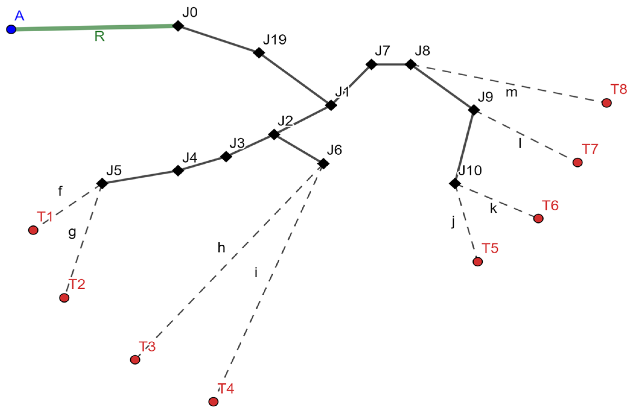
2. Problem Formulation

The WDN system under consideration here is a branched network and does not contain any loops. Nodes could be sources, junction points, or demand nodes. The variables and parameters are related by linear (material balance) and nonlinear equations (pressure drop equations). We assume that all demand flows are measured and hence all flows in the branched network can be estimated from the demand flows. For each demand node, we can formulate a pressure drop equation starting from the reservoir to the tank via all the pipes.

$$\mathit{f}\left({\mathit{z}}_{\mathbf{1}},\dots ,{\mathit{z}}_{\mathit{n}},{\mathit{b}}_{\mathbf{1}},\dots ,{\mathit{b}}_{\mathit{n}}\right)=\mathbf{0}$$

(1)

Here, $z={\left({\mathit{z}}_{\mathbf{1}},\dots ,{\mathit{z}}_{\mathit{n}}\right)}^T$ represents the variable and $b={\left({\mathit{b}}_{\mathbf{1}},\dots ,{\mathit{b}}_{\mathit{n}}\right)}^T$ represents the parameters. We consistently regard measurements as the sum of true values and a certain error. Here, the error is assumed to have a zero mean and a known positive definite covariance matrix ${\mathit{V}}_{\mathit{i}}$. In practical terms, all the values in the error are considered uncorrelated and so we consider ${\mathit{V}}_{\mathit{i}}$ as the identity matrix. If ${\tilde{\mathit{z}}}_{\mathit{i}\mathit{j}}$ is the measured value, ${\mathit{z}}_{\mathit{i}\mathit{j}}$ is the true value and ${\mathsf{ϵ}}_{\mathit{i}\mathit{j}}$ is error in that measurement in the j^th variable in the i^th experiment:

$${\tilde{z}}_{ij}=z_{ij}+{\mathsf{ϵ}}_{ij},\hspace{1em}i=1,2,\dots ,m,\hspace{1em}j=1,2,\dots ,n$$

(2)

Hence, we have ${\mathit{ϵ}}_{\mathit{i}\mathit{j}}$ = ${\tilde{\mathit{z}}}_{\mathit{i}\mathit{j}}$ − ${\mathit{z}}_{\mathit{i}\mathit{j}}$ and we can estimate the parameter b by minimizing the error norm function

$$Q\left(\mathit{b},{\mathit{z}}_{\mathbf{1}},\dots ,{\mathit{z}}_{\mathit{m}}\right)=\sum _{i=0}^m{\left(\widetilde{{\mathit{z}}_{\mathit{i}}}-{\mathit{z}}_{\mathit{i}}\right)}^{\mathit{T}}{\mathit{V}}_{\mathit{i}}^{-1}\left(\widetilde{{\mathit{z}}_{\mathit{i}}}-{\mathit{z}}_{\mathit{i}}\right),s.t.\left(1\right)$$

(3)

subjected to constraints, i.e., pressure drop equations

$$\mathit{f}\left({\mathit{z}}_{\mathit{i}},\mathit{b}\right)=0,\hspace{1em}i=1,2,\dots ,m$$

(4)

3. Estimation Algorithm

The parameters to be estimated are the major and minor loss coefficients, which are denoted by ${\mathrm{c}}_{\mathit{m}\mathit{j}}$ and ${\mathrm{c}}_{\mathit{m}\mathit{n}}$, respectively. We assume that all demand flows are measured and hence all flows in the branched network can be estimated. In the interest of clarity, we assume that the major and minor loss coefficients are the same for all the pipes and demand nodes. This is not a serious limitation and can be relaxed. The constraints in (1) arise from the nonlinear pressure drop equation, which are of the form:

$$H_s-c_{mn}\cdot {\left(d_i\right)}^2-\sum _{k\in P_i}\left({\displaystyle \frac{10.67L_k}{D_k^{4.85}}}\right){\left(Q_k\right)}^{1.85}{c}_{mj}=0$$

(5)

where H_s is the source head, d_i is the measured outflow from the i^th demand node, ${\mathrm{P}}_{\mathit{i}}$ are the set of edges (pipes) occurring in the unique path from the source to the i^th demand node, ${\mathrm{D}}_{\mathit{k}}$, ${\mathrm{L}}_{\mathit{k}}$, and ${\mathrm{Q}}_{\mathit{k}}$ are the diameter, length, and flows in the k^th edge, respectively. The algorithm operates through an iterative two-stage procedure. Initially, it commences with an initial assumption for the parameters which are updated by solving a simplified least squares problem.

$$\mathit{b}=\arg \min \sum _{\mathrm{i}=1}^{\mathrm{m}}{\left[{\mathit{f}}_{\mathit{i}}+{\mathit{J}}_{\mathit{i}}\left(\widetilde{{\mathit{z}}_{\mathit{i}}}-{\mathit{z}}_{\mathit{i}}\right)\right]}^{\mathit{T}}{\left({\mathit{J}}_{\mathit{i}}{\mathit{V}}_{\mathit{i}}{\mathit{J}}_{\mathit{i}}^{\mathit{T}}\right)}^{-1}\left[{\mathit{f}}_{\mathit{i}}+{\mathit{J}}_{\mathit{i}}\left(\widetilde{{\mathit{z}}_{\mathit{i}}}-{\mathit{z}}_{\mathit{i}}\right)\right]$$

(6)

where f_i = f(z_i,b) $f_{\mathit{i}}=f(z_{\mathit{i}},b)$ and $J_{\mathit{i}}$ is the Jacobian with respect to variables $z_{\mathit{i}}$. Subsequently, the estimates of the measured variables are updated as follows:

$${\mathit{z}}_{\mathit{i}}^{\mathit{n}\mathit{e}\mathit{w}}=\widetilde{{\mathit{z}}_{\mathit{i}}}-{\mathit{V}}_{\mathit{i}}{\mathit{J}}_{\mathit{i}}^{\mathit{T}}{\left({\mathit{J}}_{\mathit{i}}{\mathit{V}}_{\mathit{i}}{\mathit{J}}_{\mathit{i}}^{\mathit{T}}\right)}^{-1}\left({\mathit{f}}_{\mathit{i}}+{\mathit{J}}_{\mathit{i}}\left(\widetilde{{\mathit{z}}_{\mathit{i}}}-{\mathit{z}}_{\mathit{i}}\right)\right)$$

(7)

The procedure is repeated until convergence. The values obtained at convergence are then regarded as the final estimates for both flow rates and parameters. This iterative process can be facilitated through three distinct functions: one for managing the flow matrix, another for handling parameters, and a third for error calculation, which serves as the termination criterion. A web application developed in Python is under development.

4. Results

The method is demonstrated using data generated from an experimental facility [2]. The network topology is as shown in Figure 1. An overhead tank serves as the source and water is delivered to the demand nodes using a network of pipes by gravity. Continuous control valves, direct-acting solenoid valves and reverse-acting solenoid valves are employed to control the flow of water in the setup. The outflow from each of the demand nodes drains into tanks which are fitted with ultrasonic-level sensors. The outflow is estimated from the change in level of the water in the tanks. The inputs to the algorithm include the network topology and the estimated flow rates. The experiment is repeated for different valve configurations, i.e., some valves to the demand nodes are turned off. The results of the parameter estimation algorithm are presented in

Table 1. Comparison of the initial guess of the parameters and the estimated parameter.

Parameters	Initial Guess	Estimated Parameter
Major Loss Coefficient	$6.46\times {10}^9$	$4.80\times {10}^9$
Minor Loss Coefficient	$8.24\times {10}^{-5}$	$1.35\times {10}^{-4}$

. The measured and predicted flow rates (for one valve configuration with all valves open) are shown in

Table 2. Comparison of flow rates.

	T1	T2	T3	T4	T5	T6	T7	T8
Measured	12.58	17.25	15.34	23.12	9.83	6.11	0.24	0.02
Computed	11.61	20.95	17.99	24.54	7.40	3.143	0.23	0.27

All values are in 10⁻⁵ lpm.

.

5. Conclusions

This paper describes a computationally efficient method for estimating the parameters concerned with the water distribution system. The proposed approach addresses the challenges associated with errors in variables by implementing a systematic, iterative procedure. The algorithm is seamlessly automated through a Python-based software package. This work can be extended to loop networks, intermediate pressure measurements, and the partial opening of valves. Also, the parameters of pipes like the age, diameter, etc., of the pipe can be considered in the parameter estimation procedure.

References

1. Valkó, P.; Vajda, S. An Extended Marquardt-Type Procedure for Fitting Error-in-Variables Models. Comput. Chem. Eng. 1987, 11, 37–43. [Google Scholar] [CrossRef]
2. Mohandoss, P. Monitoring, Scheduling and Leak Detection in Water Distribution Networks. Master’s Thesis, Indian Institute of Technology Madras, Chennai, India, 2020. [Google Scholar]
Figure 1. This is an example of a network in the form of a tree. The red-colored nodes are the demand nodes and the black-colored nodes are the intermediate junctions. The black lines are the intermediate pipes and the dotted lines are the pipes containing valves.
Engproc 69 00145 g001