Exploring the Impact of Pulsed Demand Model on the Quality Sensor Placement in Water Distribution Networks ^†

Abstract

In this work, the impact of the actual pulsed nature of demand on the water quality sensor placement problem was investigated. The optimization was carried out by minimizing alternatively the extent of contamination and exposed population to ingestion by considering two alternative demand modelling conditions: (i) a smooth top-down deterministic approach (TDA), and (ii) a pulsed demand bottom-up stochastic approach (BUA). An Italian water distribution network was tested, and results show that the contamination extension and sensor locations are affected by demand modeling and that monitoring system performance may be overestimated if the deterministic approach is used, leading to dangerous management choices.

1. Introduction

Water distribution networks (WDNs) are critical infrastructures for the population’s prosperity. However, due to their large size, they are vulnerable to intentional/accidental contaminations, and the consequences could be harmful for thousands of people.

The installation of water quality sensors (WQSs) represents an effective strategy for securing WDNs against contaminations [1], providing early detection of risk conditions. Due to budget constraints, the most suitable locations for a limited number of WQSs must be identified, as trade-off between detection reliability and investment cost. In this regard, the optimal WQS placement problem in WDNs has been profoundly explored [2].

The reliability of the hydraulic/water quality models still represents a challenge, and the adoption of simplified models for the estimation of the distribution of contaminants may result in inefficient WQS layout. For example, nodal demands are usually estimated with bills, and a single demand pattern is assigned to the whole network. This simplification may fail to predict the fate of contaminants moving through WDNs [3]. Finer temporal/spatial resolutions should be considered due to the pulsed nature of demand [4] resulting in a higher frequency of zero demand values and flow reversals.

2. Materials and Methods

2.1. Demand Modelling

Two different approaches were considered as input to the hydraulic/water quality analysis and sensor placement for the assessment of nodal demands for the WDN modelling: (i) a top-down deterministic approach (TDA), according to which the nodal demands are obtained by multiplying the average nodal demands by a time-varying coefficient, based on billed consumption; and (ii) a bottom-up stochastic approach (BUA), which reconstructs nodal demands starting from individual users’ consumption.

For the application of the BUA, the cor-PRP model proposed by [5] was used for demand generation at the generic node, according to which the frequency of nodal residential water use follows a nonstationary Poisson arrival process. The probability Pr of having exactly k pulses generated during a time period of duration Δτ [s] is given by the following:

$$Pr\left(k\right)=e^{-\lambda \Delta \tau }{\displaystyle \frac{{\left(\lambda \Delta \tau \right)}^k}{k!}},$$

(1)

where parameter λ [s−1] is the mean pulse arrival frequency, assumed to be constant during Δτ. To improve pulse consistency, the correlation between pulse duration and intensity is also considered. After pulses were generated at the node (simulating the open faucets of the households connected to the generic node), they were aggregated at a time step of 5 min in order to obtain the nodal demand as the sum of the intensities I of all the simultaneously active pulses.

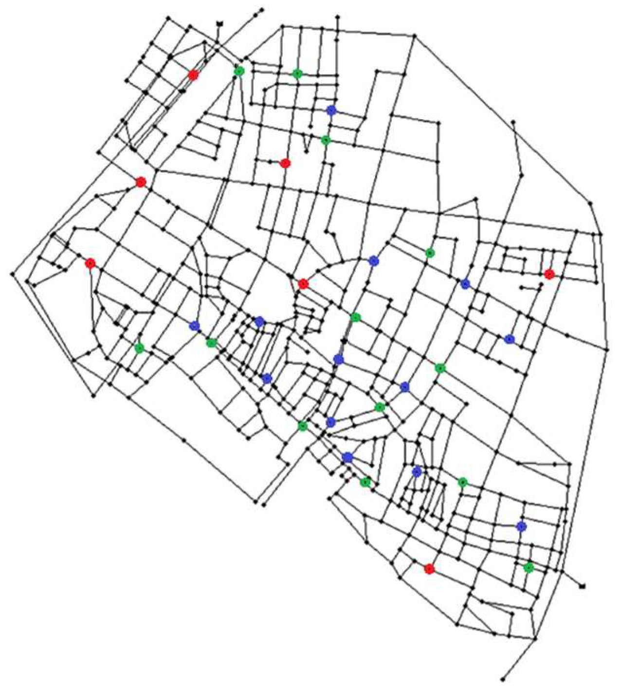
2.2. Water Quality Sensor Placement

Two kinds of optimization were run to search for WQS locations in the WDN:

• the first kind was aimed at minimizing simultaneously the number f₁ = N_sens [-] of installed sensors and the extent f₂ = EC = mean(L_c,s) [m] of contamination, where L_c,s [m] is the total length of the contaminated pipeline during a contamination scenario s at the time of the first detection;
• the second kind was aimed at minimizing simultaneously f₁ and the population f₃ = P = mean(p_s) [-] exposed to ingestion, where p_s [-] is the number of people that ingested contaminated water in the contamination scenario s at the time of the first detection, considering the five-fixed-times ingestion model [6].

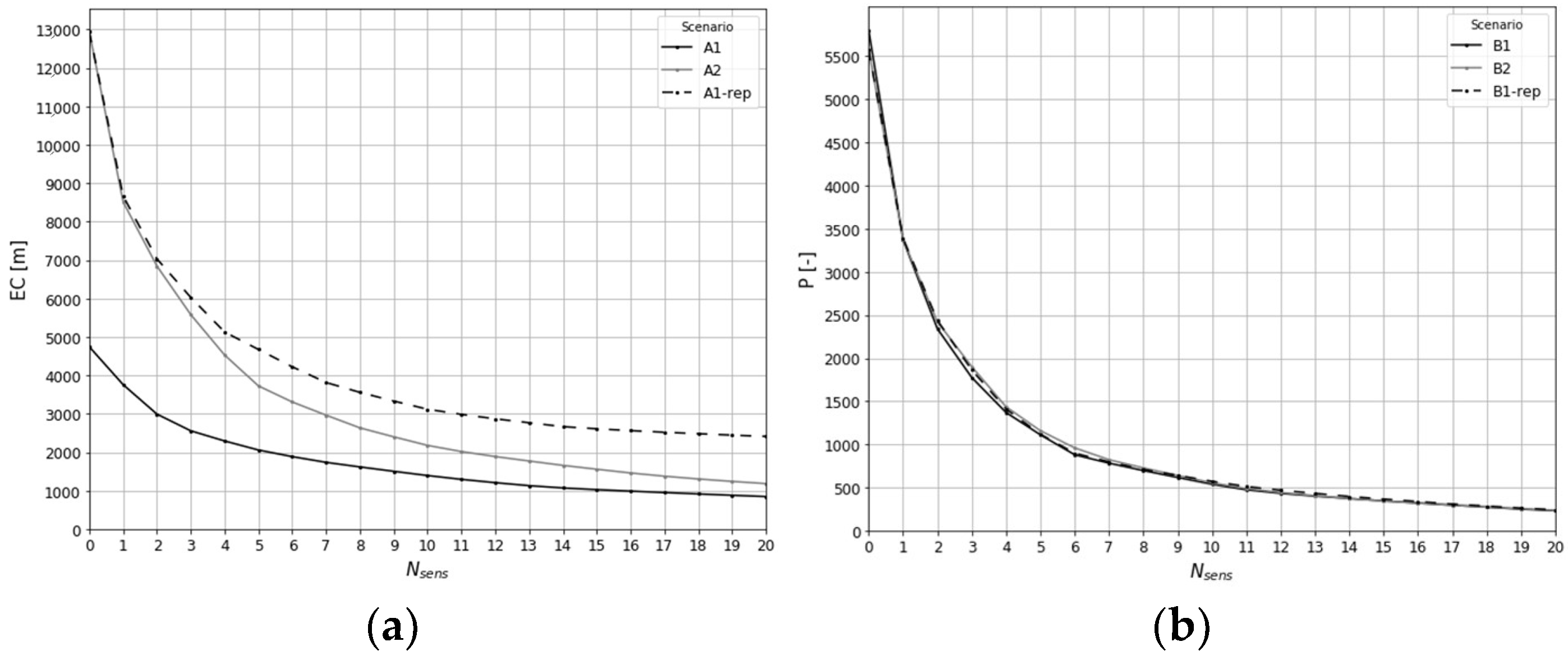
The set S of contamination events for the WQS layout design was arranged by considering the following: (i) all the nodes and the reservoirs, one by one, as locations for contaminant injection; (ii) the contamination starting time at every 15 min; (iii) one single value of the mass injection rate (100 g/min); and (iv) one single value of the injection duration (60 min). The TEVA-SPOT 2.3.1 software developed by the US EPA [7] was used for the optimizations. Finally, the obtained WQS layouts were compared using functions f₂, f₃, and f₄ = Ps = Σd_s/S [-] (Detection likelihood), where d_s = 1 if the generic contamination scenario s is detected, and d_s = 0 if otherwise. The hydraulic/water quality simulations were carried out at 5 min time step for a total extended period duration of 72 h and in demand-driven approach.

3. Results

The procedure was tested on an Italian WDN [8] composed of 536 demand nodes, 825 pipes, and two source nodes, with a total average demand of 173 L/s, and a percentage of leakage around 20%. The optimizations were organized as follows:

-

Scenario A1: EC as second objective function, TDA for the nodal demand;

-

Scenario A2: EC as second objective function, BUA for the nodal demand;

-

Scenario B1: P as second objective function, TDA for the nodal demand;

-

Scenario B2: P as second objective function, BUA for the nodal demand;

Finally, Scenario A1 and Scenario B1 were reprocessed (A1-rep and B1-rep, respectively) considering BUA for the nodal demand for the water quality simulations.

The Pareto fronts show decreasing values of objective functions as N_sens increases. When P is used for the optimization (Figure 1b), the trends are quite close, while, when EC is used for the optimization (Figure 1a), the trends are very different. For the Scenario A1, the extent of contamination is always much smaller than the Scenario A2 and A1-rep, so, if the TDA is considered, the impact of the contamination is underestimated.

In Figure 2, the WQS layouts for the case of N_sens = 20 for the Scenario A1 (green dots) and A2 (blue dots) are shown on a WDN map, with only a few locations (red dots) for the WQSs in common for the two scenarios (7 out of 20).

Scenario A1 (EC = 852) features a higher value of the exposed population (P = 429) and a lower detection likelihood (Ps = 54.7%) than Scenario A2 (EC = 1189) (P = 302 and Ps = 74.5%). Scenario A1-rep (EC = 2416) shows the lowest value detection likelihood (Ps = 53.8%) and the highest value of the exposed population (P = 439).

4. Discussion

Results of this investigation show that demand modeling impacts on the results of WQ simulations/WQS optimizations, but the extent of the influence depends on the objective function adopted. The extent of the contamination is underestimated for the TDA-based models, and the performance of the WQS layouts, from this viewpoint, was consequently overestimated in comparison with BUA, making the adoption of a more realistic demand modeling crucial. If the exposed population is used for the optimization, the performance of WQS layouts is more similar, maybe due to resulting sensor locations (more concentrated in the WDN center) where the impact of demand modeling is smaller. Deeper investigations and further discussion of findings can be read in the full journal version [9].

References

1. Giudicianni, C.; Herrera, M.; Di Nardo, A.; Creaco, E.; Greco, R. Multi-criteria method for the realistic placement of water quality sensors on pipes of water distribution systems. Environ. Model. Softw. 2022, 152, 105405. [Google Scholar] [CrossRef]
2. Adedoja, O.S.; Hamam, Y.; Khalaf, B.; Sadiku, R. A state-of-the-art review of an optimal sensor placement for contaminant warning system in a water distribution network. Urban Water J. 2018, 15, 985–1000. [Google Scholar] [CrossRef]
3. Blokker, E.J.M.; Vreeburg, J.H.G.; Buchberger, S.G.; Van Dijk, J.C. Importance of demand modelling in network water quality models: A review. Drink. Water Eng. Sci. 2008, 1, 27–38. [Google Scholar] [CrossRef]
4. Creaco, E.; Blokker, E.J.M.; Buchberger, S.G. Models for generating household water demand pulses: Literature review and comparison. J. Water Resour. Plan. Manag. 2017, 143, 04017013. [Google Scholar] [CrossRef]
5. Creaco, E.; Farmani, R.; Kapelan, Z.; Vamvakeridou-Lyroudia, L.; Savic, D. Considering the mutual dependence of pulse duration and intensity in models for generating residential water demand. J. Water Resour. Plan. Manag. 2015, 141, 04015031. [Google Scholar] [CrossRef]
6. Davis, M.J.; Janke, R. Development of a probabilistic timing model for the ingestion of tap water. J. Water Resour. Plan. Manag. 2009, 135, 397–405. [Google Scholar] [CrossRef]
7. Janke, R.; Murray, R.; Haxton, T.M.; Taxon, T.; Bahadur, R.; Samuels, W.; Uber, J. Threat Ensemble Vulnerability Assessment-sensor Placement Optimization Tool (TEVA-SPOT) Graphical User Interface User’s Manual; US EPA National Homeland Security Research Center (NHSRC): Cincinnati, OH, USA, 2012; pp. 1–109.
8. Alvisi, S.; Creaco, E.; Franchini, M. Segment identification in water distribution systems. Urban Water J. 2011, 8, 203–217. [Google Scholar] [CrossRef]
9. Giudicianni, C.; Campisano, A.; Di Nardo, A.; Creaco, E. Pulsed Demand Modeling for the Optimal Placement of Water Quality Sensors in Water Distribution Networks. Water Resour. Res. 2022, 58, e2022WR033368. [Google Scholar] [CrossRef]
Figure 1. Pareto front of optimal WQS solutions, in the trade-off between number of sensors (Nsens) and the following parameters: (a) extent of contamination (EC) for Scenario A1 (TDA), A2 (BUA), and A1-rep (A1 reprocessed with BUA); (b) population exposed through ingestion (P) for Scenario B1 (TDA), B2 (BUA), and B1-rep (B1 reprocessed with BUA).
Engproc 69 00174 g001
Figure 2. WQS layouts with Nsens = 20 for the Scenario A1 (green dots) and A2 (blue dots), with common locations as red dots.
Engproc 69 00174 g002
Disclaimer/Publisher’s Note: The statements, opinions and data contained in all publications are solely those of the individual author(s) and contributor(s) and not of MDPI and/or the editor(s). MDPI and/or the editor(s) disclaim responsibility for any injury to people or property resulting from any ideas, methods, instructions or products referred to in the content.