Cascade Machine Learning Approach Applied to Short-Term Medium Horizon Demand Forecasting ^†

Abstract

This work proposes a cascade model incorporating Long–Short-Term Memory (LSTM) and Multi-Layer Perceptron (MLP), which offers a more reliable model to forecast short-term (hourly) and medium horizon (week) water demand. The MLP model integrates the previously forecasted demand with exogenous variables, functioning as a filter to enhance the accuracy of the LSTM estimation. The LSTM model estimates, utilizing a univariate approach, the hourly forecasting of water demand for the entire available dataset and the minimum night flow. The algorithm considers various time series sizes for each DMA and predicts the water demand values for each hour throughout the week. Having forecasted all timesteps with the LSTM, a virtual online process can be implemented to enhance forecasting quality.

1. Introduction

Driven by population growth and urbanization, coupled with climate variability, efficient water resource management is critical. Demand forecasting is a growing field that, by analyzing historical data, demographic trends, climatic factors, and socio-economic variables, tries to estimate the future consumption of water in a system [1]. One such approach involves the assimilation of hydraulic observations and the estimation of water demands in real-time.

The last advances in water demand forecasting rely on the application of deep learning algorithms such as Long–Short-Term Memory (LSTM) [2] and Graph Convolutional Recurrent Neural Networks (GCRNN) [3]. LSTM captures temporal dependencies, while GCRNN combines graph-based modelling with recurrent networks to capture spatial and temporal dependencies among water demand time series. These models offer promising solutions for accurate forecasting intending to enhance water distribution system management.

To improve the accuracy of the forecasting process even more, cascade deep learning models represent a class of neural network architectures that operate sequentially, where the output of one layer or module serves as the input to the next. These cascades enable hierarchical feature extraction and progressively refine predictions. In this sense, considering the challenges of the real-time forecasting problem proposed by the Battle of Water Demand Forecasting (BWDF), this work presents a cascade deep learning approach. Water demand and minimum night flow are individually forecasted by an LSTM model. After that, exogenous variables are incorporated into the demand forecasting process using an MLP, which includes forecasted demand and minimum night flow, datetime information (day, hour, holidays), and weather information.

2. Methodology

2.1. Data Imputation

The imputation process for handling missing data is the first step to guarantee the effective application of machine learning algorithms. Missing data can introduce biases, reduce the representativeness of the dataset, and hinder the performance of machine learning models. For the dataset provided by the Battle of Water Demand Forecasting (BWDF), the inflow and weather datasets have missing values that should be handled before the application of machine learning algorithms. In our methodology, the K-Nearest Neighbor (KNN) algorithm is used for handling missing data, as proposed by [4]. The algorithm works by finding the nearest samples in the dataset to the missing values and averaging them. The following two key parameters must be selected for optimal performance: the number of neighbours used for averaging and the distance metric for calculating proximity. In this study, a simple search between 1 and 100 was conducted to determine the number of neighbours, while the Euclidean distance metric was employed, which is commonly utilized.

2.2. Long Short Term Memory (LSTM)

Long–Short-Term Memory (LSTM) networks stand as a subclass of recurrent neural networks (RNNs) that are highly regarded for their capability of managing sequential data [5]. The use of memory units operated by gates that can input, forget, and output data on the learning process is the key point that makes LSTMs powerful when compared with other recurrent networks. These gates empower selective modifications to the internal memory state, thus enabling the representation of temporal patterns. A critical feature of an LSTM is the mitigation of vanishing and exploding gradient problems encountered in traditional Recurrent Neural Networks (RNNs), thereby enabling effective learning and the retention of sequential patterns over long sequences [6]. The key components of an LSTM unit include the input gate, the forget gate, the output gate, and the cell state, each of which is governed by various learned parameters.

2.2.1. Water Demand Forecasting

The LSTM is trained over all the demand sequences of all DMAs to predict only one step ahead (1 h). The input of the model is composed of a sequence of $n$ measured values, being the number of DMAs. Each sequence has a pre-defined length that is composed by the lags with higher autocorrelation. In our study, the lags correspond to 168, 167, 144, 143, 24, 23, 22, 3, 2, and 1 h. This means that the LSTM takes as input the t-1, t-2, t-3, t-22, … t-168 observation of all the DMAs to simultaneously predict 1 h ahead of all the time series. Given that we have 10 DMAs in the BWDF (A to J), the inputs are 10 sequences of 10 lags (100 numbers), while the outputs are 1 step ahead for all the DMAS (10 numbers).

2.2.2. Minimum Night Flow Forecasting

The minimum night flow is predicted by an LSTM model on daily time resolution. This model utilizes the water demand of the previous day, along with the month number, weekday, forecasted precipitation sum, and forecasted mean temperature of the considered day as input features. Therefore, an LSTM model is created and tuned for each day in the prediction horizon and each DMA, resulting in 70 independent LSTM models. The LSTM models for minimum night flow are implemented in Python using PyTorch. The LSTM architecture consists of two layers, whereas the number of neurons for each layer, the learning rate, and the batch size are automatically pre-tuned for each LSTM model within the range [16, 32, 64], [10⁻⁴,10⁻⁴¹], and [2, 4, 8, 16], respectively, with a maximum of 10 epochs. Afterwards, the best configuration is selected, and the LSTM model is trained and validated using an Adam optimizer with MSE as the loss function, a dropout rate of 0.1, and a bidirectional setting.

2.3. Cascade Approach

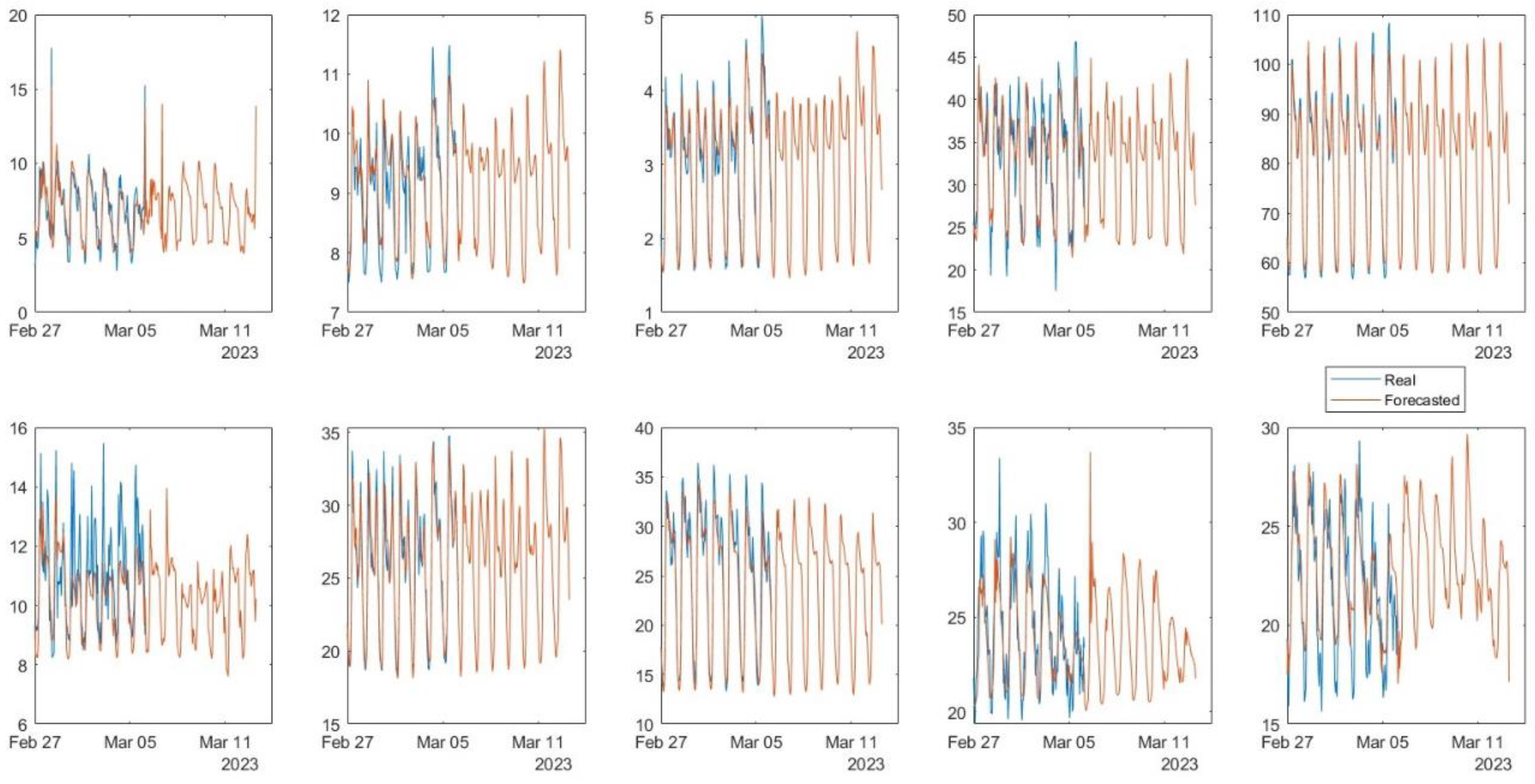
After obtaining the water demand forecasts from the LSTM model, a second forecasting step is performed to improve the results further. This additional layer incorporates external factors that influence water demand, essentially acting as a correction mechanism for the LSTM forecasts. Following the creation of the new dataset, the architecture of the Multi-Layer Perceptron (MLP) is optimized using a grid search algorithm. This algorithm explores different configurations by varying the number of hidden layers (2 to 4) and the number of neurons within each layer (5 to 50). Due to the sensitivity of the MLP algorithm to initial parameters, each grid search is executed 20 times to identify the configuration that minimizes error.

3. Results

The results of this work are evaluated according to the Battle of Water Demand Forecasting (BWDF) indicators, presented at https://wdsa-ccwi2024.it/battle-of-water-networks/ (accessed on 1 January 2024). Those indicators measure the absolute average and maximum error for the first 24 h of prediction and the average error for the remaining hours of the evaluation week. For the training of the correction layer using MLP, the available dataset is split into two, where the last month of the dataset is used to test the global forecasting process while the remaining dataset is used for training.

Table 1. Evaluation indicators for each week of Battle of Water Demand Forecasting.

DMA	A	B	C	D	E	F	G	H	I	J
WEEK 1
Total Score	3.16	1.76	1.52	5.88	4.50	2.55	4.19	1.89	2.91	4.54
Max 24 h	1.65	0.83	0.72	3.19	2.48	1.14	2.09	0.95	1.43	2.60
Aver. 24 h	0.68	0.61	0.52	1.31	1.16	0.91	1.28	0.42	0.80	1.15
Aver. Week	0.83	0.33	0.29	1.39	0.85	0.50	0.82	0.51	0.69	0.79
WEEK 2
Total Score	7.60	1.74	1.41	8.62	10.02	3.62	3.14	5.84	7.43	5.47
Max 24 h	5.09	0.85	0.79	4.53	6.44	1.99	1.66	3.20	4.36	2.16
Aver. 24 h	1.32	0.57	0.39	2.21	1.82	0.87	0.89	1.37	1.82	2.30
Aver. Week	1.20	0.33	0.23	1.87	1.77	0.75	0.59	1.28	1.25	1.01
WEEK 3
Total Score	4.39	1.59	1.63	8.82	7.75	4.73	3.25	5.84	6.01	5.47
Max 24 h	2.12	0.78	0.87	4.61	4.84	2.71	1.67	3.14	3.11	2.16
Aver. 24 h	1.36	0.47	0.52	2.25	1.66	1.03	0.95	1.38	1.83	2.30
Aver. Week	0.92	0.34	0.25	1.96	1.25	0.98	0.63	1.33	1.07	1.01
WEEK 4
Total Score	2.48	1.49	0.86	10.52	5.77	2.63	2.90	4.45	4.33	4.31
Max 24 h	1.33	0.84	0.45	6.10	2.45	1.43	1.34	2.24	2.33	2.28
Aver. 24 h	0.71	0.32	0.23	2.21	2.36	0.69	1.06	1.33	1.20	1.28
Aver. Week	0.44	0.33	0.18	2.22	0.96	0.51	0.50	0.88	0.81	0.76

shows the indicators for the 4 evaluation weeks of the test dataset.

To illustrate the behaviour of forecasted demand during the last evaluation week (W4), Figure 1 presents the forecasted and real values for all the DMAs. It is worth noting that for most of the DMAs, the forecasting values correctly follow the expected real ones. Nevertheless, mainly for DMA F and DMA J, the forecasting algorithms are not able to achieve the maximum demand, leading to a high percentage error.

References

1. Barzegar, R.; Aalami, M.T.; Adamowski, J. Short-term water quality variable prediction using a hybrid CNN–LSTM deep learning model. Stoch. Environ. Res. Risk Assess. 2020, 34, 415–433. [Google Scholar] [CrossRef]
2. Zanfei, A.; Brentan, B.M.; Menapace, A.; Righetti, M. A short-term water demand forecasting model using multivariate long short-term memory with meteorological data. J. Hydroinform. 2022, 24, 1053–1065. [Google Scholar] [CrossRef]
3. Zanfei, A.; Brentan, B.M.; Menapace, A.; Righetti, M.; Herrera, M. Graph convolutional recurrent neural networks for water demand forecasting. Water Resour. Res. 2022, 58, e2022WR032299. [Google Scholar] [CrossRef]
4. Zanfei, A.; Menapace, A.; Brentan, B.M.; Righetti, M. How does missing data imputation affect the forecasting of urban water demand? J. Water Res. Plan. Manag. 2022, 148, 04022060. [Google Scholar] [CrossRef]
5. Hochreiter, S.; Schmidhuber, J. Long short-term memory. Neural Comput. 2018, 9, 1735–1780. [Google Scholar] [CrossRef] [PubMed]
6. Mikolov, T.; Joulin, A.; Chopra, S.; Mathieu, M.; Ranzato, M.A. Learning longer memory in recurrent neural networks. In Proceedings of the International Conference on Learning Representations, San Diego, CA, USA, 8 May 2015. [Google Scholar]
Figure 1. Results of the proposed methodology in weekly water demand forecasting on the 10 DMAs.
Engproc 69 00042 g001