Real-Time Demand Forecasting and Multi-Resolution Model Predictive Control for Water Distribution Networks ^†

Abstract

In this work, we develop a water demand prediction model for MPC that reliably handles unexpected changes from the daily pattern by incorporating a dynamical model over the current measured demand, fitted using machine learning methods. Secondly, in alignment with the new demand estimator, we also propose a multi-resolution MPC prediction horizon. This improves the responsiveness to unforeseeable disturbances with minimal impact on computational efficiency.

1. Introduction

Water distribution networks (WDNs) are large-scale systems that supply drinking water to consumers over a large area. However, WDNs are subject to increasing uncertainties because of climate change, a growing economy/population, and the rapid transition to renewable energy sources. Addressing these uncertainties in future water networks necessitates an adaptive (pump) scheduling method. One of the most suitable scheduling methods is model predictive control (MPC) [1,2], which can take the physical limits of the WDN into account and can provide optimal scheduling strategies. Nonetheless, MPC requires an accurate prediction model, and, as such, it relies on accurate water demand forecasting. Water demand is often modeled as a time series with a daily or weekly pattern, based on the demographics at the demand node location [3] and/or historical demand data, if available. While providing a robust mean demand, these prediction models cannot predict real-time changes [4].

In this work, we develop a water demand prediction model for MPC that reliably handles unexpected changes from the daily pattern by incorporating a dynamical model over the current measured demand, fitted using machine learning methods, including the Auto-Regressive (AR) model, Recurrent Neural Networks (RNNs), and Multi-Layer Perceptron (MLP). This is initiated by analyzing data generated by SIMDEUM [3]. From autocorrelation test results, we show that the developed dynamical models do not improve the prediction accuracy beyond 2 h. Therefore, we introduce a novel MPC design for WDNs that uses a multi-resolution horizon. In the standard formulation of MPC for WDNs, a 24 h prediction horizon is used with a sampling period of 1 h. The multi-resolution formulation we propose uses a sampling period of 10 min for the first 2 h, and then, the usual 1 h sampling interval is used for the remaining 22 h. The resulting control law allows the closed loop to be evaluated every 10 min while keeping the corresponding control problem size minimal.

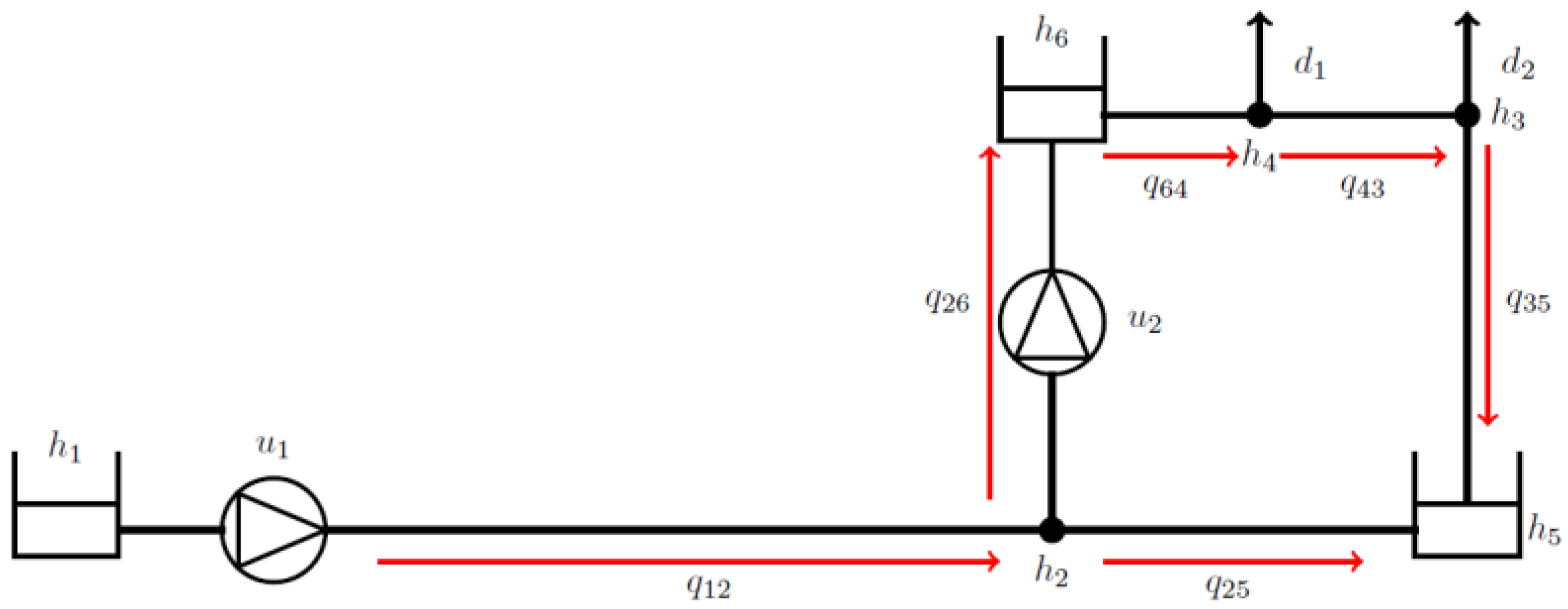
2. Control Architecture with Demand Prediction

Water distribution networks can be described by four basic elements: pipes, nodes, storage tanks, and actuators such as pumps or controllable valves. The resulting model and the derivation of this model that we will use in this brief paper are illustrated in [5]. The demand nodes represent the locations in the network where water leaves the network.

Figure 1 shows the simple water network we consider. It has two demand nodes in a gravity line between tank $h_6$ and $h_5$. The control law is the result of the following MPC problem:

$$\begin{array}{c}\underset{X_k}{\min }{\displaystyle \sum _{i=0}^{N-1}}{\mathsf{\lambda }}_1{l}_1\left(k+i\right)+{\mathsf{\lambda }}_2{l}_2\left(k+i\right)+{\mathsf{\lambda }}_3{l}_3\left(k+i\right)\hfill \\ s.t. x_{0|k}=x\left(k\right)\hfill \\ g\left(x_{i|k}\right)\le 0, h\left(x_{i|k}, d_{i|k}\right)=0 \forall i\in 0,\dots ,N-1\hfill \end{array}$$

where cost terms $l_1$, $l_2$, and $l_3$ represent the safety head cost, pump switching cost, and pump electricity cost, respectively [5]. The optimization vector $X_k$ concatenates $x_{i|k}$ over prediction horizon N, where each $x_{i|k}$ contains the network flows, nodal and tank heads, and control inputs. The resulting control flow (i.e., the pump flow) will be set as a setpoint for underlying pump controllers.

The demand flow $d_{i|k}$ is predicted as $d_{i|k}=d_{\mathrm{base}}\left(k+i\right)+d_{\mathrm{NN}}\left(k+i\right),$the sum of baseline demand data and an offset, which is obtained by a neural network that anticipates future demand changes based on past-window demand data. The baseline demand $d_{\mathrm{base}}\left(k\right)$ can be obtained by averaging over a long window of historical data. The baseline can also be unique per day and change seasonally, improving accuracy for the expected occasion but, in turn, requiring much more data for a reliable fit. Figure 2a shows the residual correlation between the current demand and the (actual) future demand, both with the baseline subtracted.

The strong correlation for small lags (less than 25) indicates that there is a residing dynamical component that, through the correlation with the current measurements, can be estimated as well. This is where $d_{\mathrm{NN}}\left(k+i\right)$ will play a role.

Demand Estimation Using Artificial Intelligence

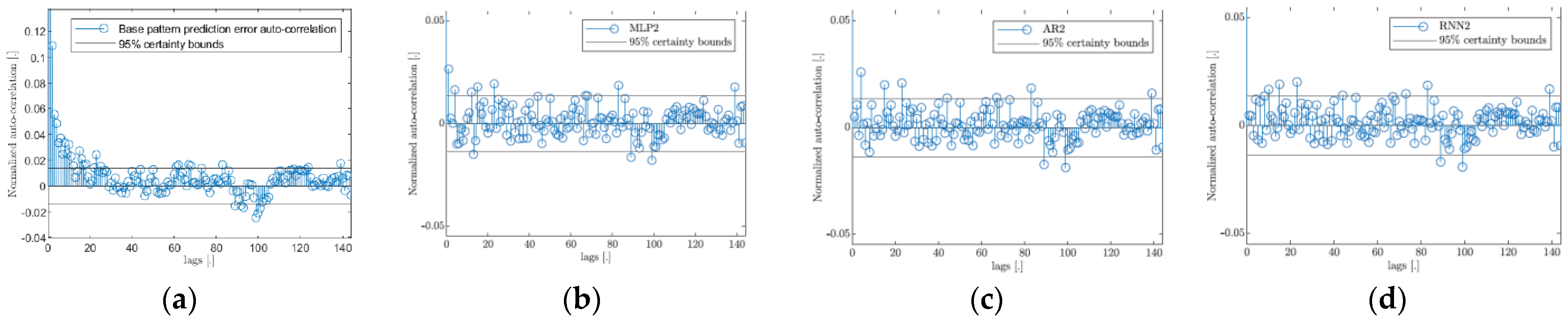
While demand is mostly periodic, small offsets reduce the optimality of the selected pump settings. We seek to reduce the impact of these demand mismatches by predicting a short window of demand offset using a short window of past data (with the idea that measured mismatches can be expected to continue in the near future). For this, we considered different types of AI models, shown in

Table 1. AI methods tested for real-time demand prediction.

Auto-Regressive (AR)	Recurrent Neural Network (RNN)	Multi-Layer Perceptron (MLP)
$x_{\mathrm{out}}=W{x}_{in}$	$z_{\mathrm{t}}={\sigma }_g\left(W_z{x}_{in}+U_z{h}_{t-1}+b_z\right)$ $r_t={\sigma }_g\left(W_r{x}_{in}+U_r{h}_{t-1}+b_r\right)$ ${\widehat{h}}_t={\varphi }_h(W_h{x}_{in}+U_h\left(r_t\circ h_{t-1}\right)+b_h$ $h_t=z_t\circ h_{t-1}+\left(1-z_t\right)\circ {\widehat{h}}_1$ $x_1=f_{RELU}\left(W_1{h}_t+b_1\right)$ $x_{out}=W_{out}{x}_1+b_{out}$	$x_1=f_{RELU}\left(W_1{x}_{in}+b_1\right)$ $x_2=f_{RELU}\left(W_2{x}_1+b_2\right)$ $x_3=f_{RELU}\left(W_3{x}_2+b_3\right)$ $x_{out}=W_{out}{x}_3+b_{out}$

. The exact dimensions of the selected methods and their complete explanation can be found in [6].

The data used to train the models are generated by SIMDEUM, considering a time window of 500 days at a 10 min sampling interval. These data are normalized by

$$x_{train}\left(k\right)={\displaystyle \frac{d\left(k\right)-d_{\mathrm{b}\mathrm{a}\mathrm{s}\mathrm{e}}\left(k\right)}{\sigma \left(k\right)}},$$

where $\mathsf{\sigma }\left(k\right)$ is the standard deviation at time-of-day instance $k$. Given that the autocorrelation in Figure 2a only details a noticeable correlation in the first lags, these models will only predict the next 14 demand offsets. The autocorrelations of the three AI methods are shown in Figure 2b–d, where a clear reduction in the initial correlation is visible.

In earlier work, [5] showed that the MPC law for WDNs is more efficient for sampling periods shorter than 1 h (the “standard” sampling period [1]). However, the resulting increase in prediction horizon reduces computational efficiency. Now, since the demand prediction can only be improved for the next 140 min, we propose a multi-resolution sampling-period prediction horizon. The first 2 h are predicted at a 10 m interval and the remaining 22 h at 1 h intervals. This increases the total prediction horizon by only 10 (from 24 to 34) and changes the online sampling interval to 10 m, thus yielding a faster response time to unforeseeable events. In the end, we develop the following MPC control law:

$$\begin{array}{c}\underset{X_k}{\min }{\displaystyle \sum _{i=0}^{N_s-1}}{\mathsf{\lambda }}_1{l}_1\left(k+i\right)+{\mathsf{\lambda }}_2{l}_2\left(k+i\right)+{\mathsf{\lambda }}_3{l}_3\left(k+i\right)\hfill \\ \hspace{1em}\hspace{1em}\hspace{1em}\hspace{1em}\hspace{1em}\hspace{1em}\hspace{1em}+{\displaystyle \sum _{i=0}^{(N-N_s)/T_m}}{\mathsf{\lambda }}_1{l}_1\left(k+N_s+i{T}_m\right)\hfill \\ \hspace{1em}\hspace{1em}\hspace{1em}\hspace{1em}\hspace{1em}\hspace{1em}\hspace{1em}+{\mathsf{\lambda }}_2{l}_2\left(k+N_s+i{T}_m\right)+{\mathsf{\lambda }}_3{l}_3\left(k+N_s+i{T}_m\right)\hfill \\ s.t. x_{0|k}=x\left(k\right)\hfill \\ g\left(x_{i|k}\right)\le 0, \forall i\in 0,\dots ,N_s-1\hfill \\ h\left(x_{i+1|k},x_{i|k}, d_{i|k}\right)=0, \forall i\in 0,\dots ,N_s-1\hfill \\ g\left(x_{i|k}\right)\le 0, \forall i\in N_s,N_s+T_m,\dots ,N-T_m\hfill \\ { h}_m\left(x_{i+T_m|k},x_{i|k}, d_{base}(k+i)\right)=0, \forall i\in N_s,N_s+T_m,\dots ,N-T_m\hfill \end{array}$$

where $T_m$ is the step of the larger resolution in the MPC horizon (here 6, as the sampling period is now 10 min), and $N_s$ is the short horizon’s length (12).

3. Results

To present an illustrative example, we refer to the system presented in Figure 1. In this system, we implement the multi-stepsize MPC control law with the demand generator as explained in Section 2.1. For the demand pattern, we generated demand data using SIMDEUM [3], spanning 500 days and considering 2500 demo households. Both demand nodes $d_1$ and $d_2$ in the network share this pattern, with$d_2=0.5d_1.$

The results shown in

Table 2. Six-day simulation results with different demand predictors [6].

	10 min Sampling Period			Multi-Resolution Sampling Period
	Exact	Base Only	Base + AR	Exact	Base Only	Base + AR
$l_1$ cost	70,658	70,765	70,777	70,663	70,770	70,782
$l_2$ cost	157.3	164.8	176.5	158.5	165.5	176.9
$l_3$ cost	4616	9002	7447	4821	9413	7790
Solver time	1.58s	1.56s	1.57s	0.34s	0.34s	0.34s

indicate that, indeed, using artificial intelligence methods to improve demand forecasting reduces controller costs, especially pumping cost $l_3$, compared to using averaged demand patterns (i.e., the baseline). Furthermore, the multi-resolution MPC horizon almost exactly retains controller performance but is almost five times as computationally efficient. Nonetheless, the current conclusions are based on simulated data. Real demand data are necessary to validate the algorithm in a practical scenario.

References

1. Wang, Y.; Puig, V.; Cembrano, G. Non-linear economic model predictive control of water distribution networks. J. Process Control. 2017, 56, 23–34. [Google Scholar] [CrossRef]
2. Castelletti, A.; Ficchì, A.; Cominola, A.; Segovia, P.; Giuliani, M.; Wu, W.; Lucia, S.; Ocampo-Martinez, C.; Schutter, B.D.; Maestre, J.M. Model predictive control of water resources systems: A review and research agenda. ARC 2023, 55, 442–465. [Google Scholar] [CrossRef]
3. Blokker, E.J.M.; Pieterse-Quirijns, E.J.; Vreeburg, J.H.G.; Van Dijk, J.C. Simulating Nonresidential Water Demand with a Stochastic End-Use Model. J. WRPM 2011, 137, 511–520. [Google Scholar] [CrossRef]
4. Bakker, M.; Vreeburg, J.H.G.; van Schagen, K.M.; Rietveld, L.C. A fully adaptive forecasting model for short-term drinking water demand. Environ. Model. Softw. 2013, 48, 141–151. [Google Scholar] [CrossRef]
5. Verheijen, P.C.N.; Lazar, M.; Goswami, D. Efficient Implementation and Sampling Period Analysis of MPC for Water Distribution Networks. IFAC papersOnline 2022, 55, 42–47. [Google Scholar] [CrossRef]
6. de Groot, W.P. Nonlinear Demand Prediction for Model Predictive Control of Water Distribution Networks. Master Thesis, Eindhoven University of Technology, Eindhoven, The Netherlands, 17 July 2023. [Google Scholar]
Figure 1. Sample water network with two demand nodes.
Engproc 69 00070 g001
Figure 2. The 1-step-ahead autocorrelation of the baseline demand (a) and the baseline demand combined with either an MLP (b), an AR model (c), or an RNN (d) [6].
Engproc 69 00070 g002