Efficiency Analysis of Kolmogorov-Arnold Networks for Visual Data Processing ^†

Abstract

In the field of artificial neural networks, the use of multilayer perceptrons (MLPs) has long been a well-established methodology. Recently, the theory of Kolmogorov–Arnold Networks (KANs) has emerged as a potential alternative to multilayer perceptrons, inspired by the Kolmogorov–Arnold representation theorem. It has been demonstrated that solutions based on the Kolmogorov–Arnold Network (KAN) can achieve better efficiency than those based on the multilayer perceptron (MLP) for certain problems. In this work, we investigate how the new theory can be applied to a special image classification task when some adversarial attack method is applied. The aim of the research is to explore the potential of the theory to answer the question of its applicability to complex tasks of practical importance.

1. Introduction

In recent years, neural network image processing, like classification, detection, or segmentation, has seen significant progress due to the development of machine-learning algorithms and neural network architectures. Among these advancements, Kolmogorov–Arnold Networks (KANs) [1] have become a promising approach, offering a theoretically grounded method for function approximation based on the Kolmogorov–Arnold representation theorem [2,3]. This theorem states that any continuous multivariate function can be represented as a combination of continuous univariate functions. By using this idea, Kolmogorov–Arnold Networks can break down high-dimensional data into simpler, more manageable parts. The use of KANs in image classification represents a new combination of theoretical mathematics and practical machine learning. Popular image classification methods, often based on deep convolutional neural networks (CNNs) [4,5,6], have shown impressive results, but this has led to increased complexity and computational demands [7,8,9]. KANs offer a strong alternative, providing a framework that may reduce the depth and complexity of the network needed to achieve similar accuracy. This reduction in complexity can lead to faster training times, lower computational costs, and better scalability, making KANs a good choice for large-scale image classification tasks. In this work, we explore the use and impact of KANs for a specific image classification task using different dataset attack methods. The dataset includes images of bus drivers, with the goal of detecting instances of mobile phone use while driving. The structure of our paper is as follows. Section 2 describes the mathematical and theoretical background. Section 3 details the structure of the proposed dataset. Section 4 presents the network architecture developed in this research. Section 5 details the training of neural networks and discusses the results obtained. Finally, Section 6 provides our conclusion and future outlook.

2. Kolmogorov–Arnold Network Theory

The application of the Kolmogorov–Arnold representation theorem [2,3] in the field of artificial neural networks represents a promising new area of research. It is anticipated that the proposed approach will enhance the efficiency of networks, which may in turn lead to improved solutions for specific problems. The theory of KAN [1] was developed primarily as a superior alternative to the multilayer perceptron. Therefore, it would be beneficial to undertake a comparative analysis of its efficiency with this. In the case of the multilayer perceptron, the activation functions at the neurons are fixed and non-learnable, while the learning weights between the neurons are variable. The KAN network challenges this concept. In contrast to the MLP, which employs fixed, non-learnable activation functions and learnable, linear weights, the KAN network utilizes non-linear and learnable functions. This is achieved through the use of spline functions that can be parameterized, which are then represented as learnable values within the neural network. This theorem states that any multivariate continuous function can be represented as the superposition of univariate functions. In formal terms, KAN theory asserts that there is a multivariate function:

$$f\left(x_1,x_2,\dots ,x_n\right),$$

(1)

where $n$ is the number of input parameters. Let

$$f\left(x_1,x_2,\dots ,x_n\right)={\sum }_{q=1}^{2n+1}{\mathsf{\Phi }}_q\left({\sum }_{p=1}^n{\varphi }_{q,p}\left(x_p\right)\right),$$

(2)

where $n$ is the number of inputs, $x_p$ is the $p$-th input, and ${\varphi }_{q,p}$ is a univariate function, which is mapping the inputs:

$${\varphi }_{q,p}:\left[0,1\right]\to \mathbb{R},$$

(3)

and the ${\mathsf{\Phi }}_q$ univariate function performs the following mapping:

$${\mathsf{\Phi }}_q:\mathbb{R}\to \mathbb{R},$$

(4)

For KAN networks, each layer can be represented as a matrix of these functions:

$$\mathsf{\Phi }=\left[\begin{array}{cc}\begin{array}{cc}{\varphi }_{1,1}& {\varphi }_{2,1}\\ {\varphi }_{1,2}& {\varphi }_{2,2}\end{array}& \begin{array}{cc}\cdots & \begin{array}{c}{\varphi }_{n_{out},1}\\ {\varphi }_{n_{out},2}\end{array}\end{array}\\ \begin{array}{c}⋮\\ \begin{array}{cc}{\varphi }_{1,n_{in}}& {\varphi }_{2,n_{in}}\end{array}\end{array}& \begin{array}{cc}\ddots & ⋮\\ \cdots & {\varphi }_{n_{out},n_{in}}\end{array}\end{array}\right],$$

(5)

where $n_{in}$ is the number of inputs in the given layer, and $n_{out}$ is the output features generated by that layer. Each ${\varphi }_{q,p}$, where $p=1,2,\dots ,n_{in}$ and $q=1,2,\dots ,n_{out}$, can be mapped to a B-spline function:

$$\varphi \left(x\right)=w_{b}b\left(x\right)+w_{s}s\left(x\right),$$

(6)

where $b$ is the Sigmoid Linear Unit [10] activation function:

$$b\left(x\right)=SiLU\left(x\right)={\displaystyle \frac{x}{1+e^{-x}}},$$

(7)

and $s$ is the linear combination of B-splines:

$$s\left(x\right)={\sum }_i{c}_i{B}_i\left(x\right),$$

(8)

where $c_i$ is trainable.

3. Proposed Dataset

We created a dataset comprising images of bus drivers. Each image shows the face of the bus driver while driving. For the purposes of analysis, we divided the images into two non-overlapping groups. In one case, the driver is on the phone while driving. In the other case, he is not using his phone. The images were obtained in collaboration with a partner in the passenger transportation industry. The dataset contains only images of real bus drivers talking on the phone while driving their vehicle. The final dataset contains a total of 19,552 samples. The dataset was constructed for the purpose of a classification exercise. This dataset contains information regarding the presence or absence of mobile-phone usage for each image. The dataset comprises two distinct subsets: one includes images of bus drivers while using a phone, and the other contains images of the same persons without using a mobile phone. These images were divided into two distinct sets for the purpose of training and testing. The training set contains 15,640 samples, while the test set includes $3912$ images. Figure 1 depicts images from the dataset.

The dimensions of each image are 96 pixels in height and 96 pixels in width. The images are presented in color, with three color channels within the RGB color space. Images were captured of a total of seven different bus drivers, with the following quantities: $4580$, $5302$, $1180$, $1920$, $430$, $5700$, and $440$. For each bus driver, half of the images can be classified into one category (mobile-phone usage), and the other half into the other category (no mobile-phone usage). During the preparation of the dataset, it was important to ensure that the physical appearance and behavior of the drivers involved exhibited considerable diversity. The images exclusively encompass the driver’s face and its immediate surroundings in a manner that enables a human observer to discern whether or not the driver is engaged in a phone conversation. For a given driver, the images were consistently captured from the same viewpoint. However, slight variations were observed across drivers.

4. Network Architectures

In our research, we implemented six different neural network designs. Three used KAN layers, and three did not. We aimed to create various networks with different architectures, including both simple and complex solutions. The first architecture is LinNet, which is built from two fully connected layers. The first has an input size of $n\times \mathrm{27,648}$ and an output size of $n\times 64$, where $n$ is the batch size. The second layer’s output is $n\times 2$. After that, a softmax function is used to obtain the network’s output. The first layer contains 1,769,536 parameters, and the second contains only $130$ parameters. The second network is like LinNet, but it adds a third fully connected layer. It is named LinNet L, where “L” stands for “large”. Here, the first layer’s output is $n\times 640$. The sizes of the next two layers match those of LinNet. The number of parameters in the three layers are the following: 17,695,360, $41.024$, and $130$. This network also ends with a softmax function. Our next solution is LinKAN. It is similar to LinNet, with one key difference: the last fully connected layer replaced with a KAN of the same size. The linear layer has 1,769,536 parameters, and the KAN layer has $1280$ parameters. The fourth solution is called KANNet, a purely KAN-based solution. It contains two KAN layers. The first expects an input size of $n\times \mathrm{27,648}$ and produces an output size of $n\times 64$. The second KAN layer’s output is $n\times 2$. The first KAN layer has 17,694,720 parameters, and the second has $1280$. The next solution includes a convolutional layer; this is called ConvNet, where the first layer is a convolutional filter. The convolution has $3$ input and $32$ output channels. The kernel size is $5\times 5$, and the stride value is $2$. The convolution is performed with $0$ padding and a dilation value of $1$. This layer has $2432$ parameters. It is followed by a ReLU [11] activation and a maxpool with a kernel size of $2\times 2$. After a flatten layer, the network is completed with two linear layers. The first has an input size of $n\times \mathrm{16,928}$ and an output size of $n\times 64$. The second layer’s output is $n\times 2$, with a softmax function generating the network’s output. In all cases, $n$ refers to the batch size. The linear layers have $\mathrm{1,083,456}$ and $130$ parameters. Our last implementation is also a convolution-based network, called KANConvNet. Its architecture is like ConvNet, but the linear layers at the end are replaced by KAN layers, where the first layer has 10,833,920 parameters, and the last has $1280$ parameters.

5. Results

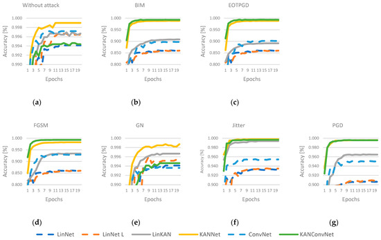
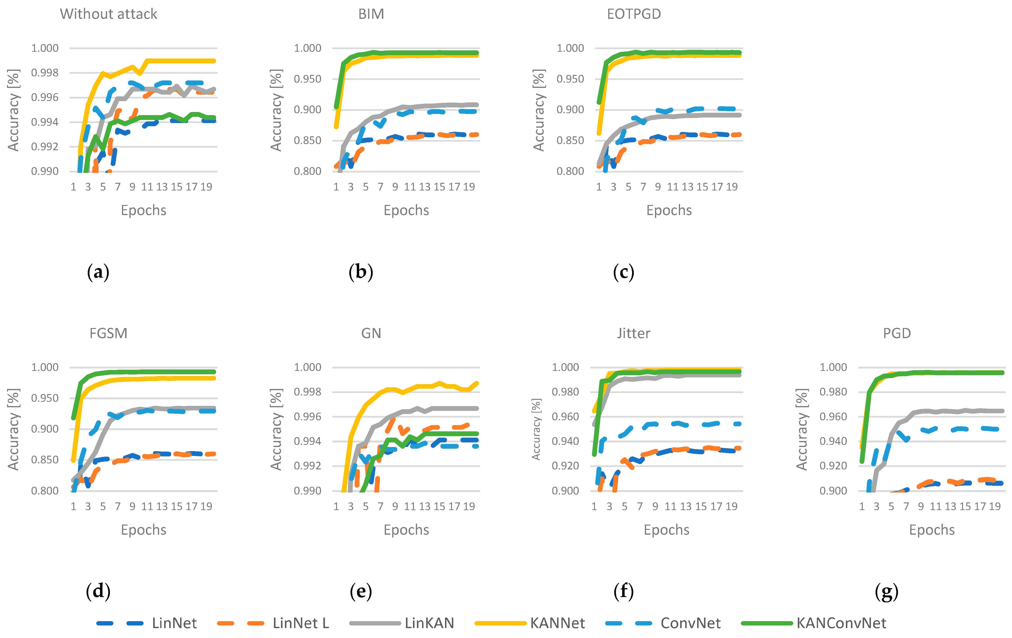
This paper presents a comparative analysis of the models described in Section 4, where the dataset described in Section 3 was used for the training. To more effectively illustrate the distinction in efficiency between MLP and KAN, adversarial attack methods were utilized. The following six attack methods were used: BIM [12], EOTPGD [13], FGSM [14], Jitter [15], PGD [16], and random Gaussian noise (GN). The adversarial attack methods were applied based on the work by Kim [17]. Each model was trained in seven ways: first without using any attack method and then with the attack methods described. In each case, the Adam optimization algorithm [18] was employed, with a learning rate value of $1\times {10}^{-4}$ and a weight decay value of the same magnitude. In the training process, the Cross-Entropy function was used to determine the loss. The accuracy values measured during the training process are presented in Figure 2. The results show that when no attack method was used, all networks performed well. In this case, the best performance was achieved using the KANNet architecture. In cases where an attack method has been used, KANNet and KANConvNet networks perform much better than the others. The exception is the GN method, which is not a targeted attack method but a random noise source, where KAN-based methods do not stand out from the other solutions.

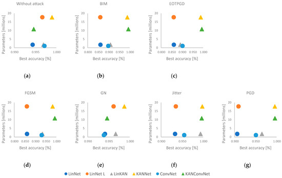
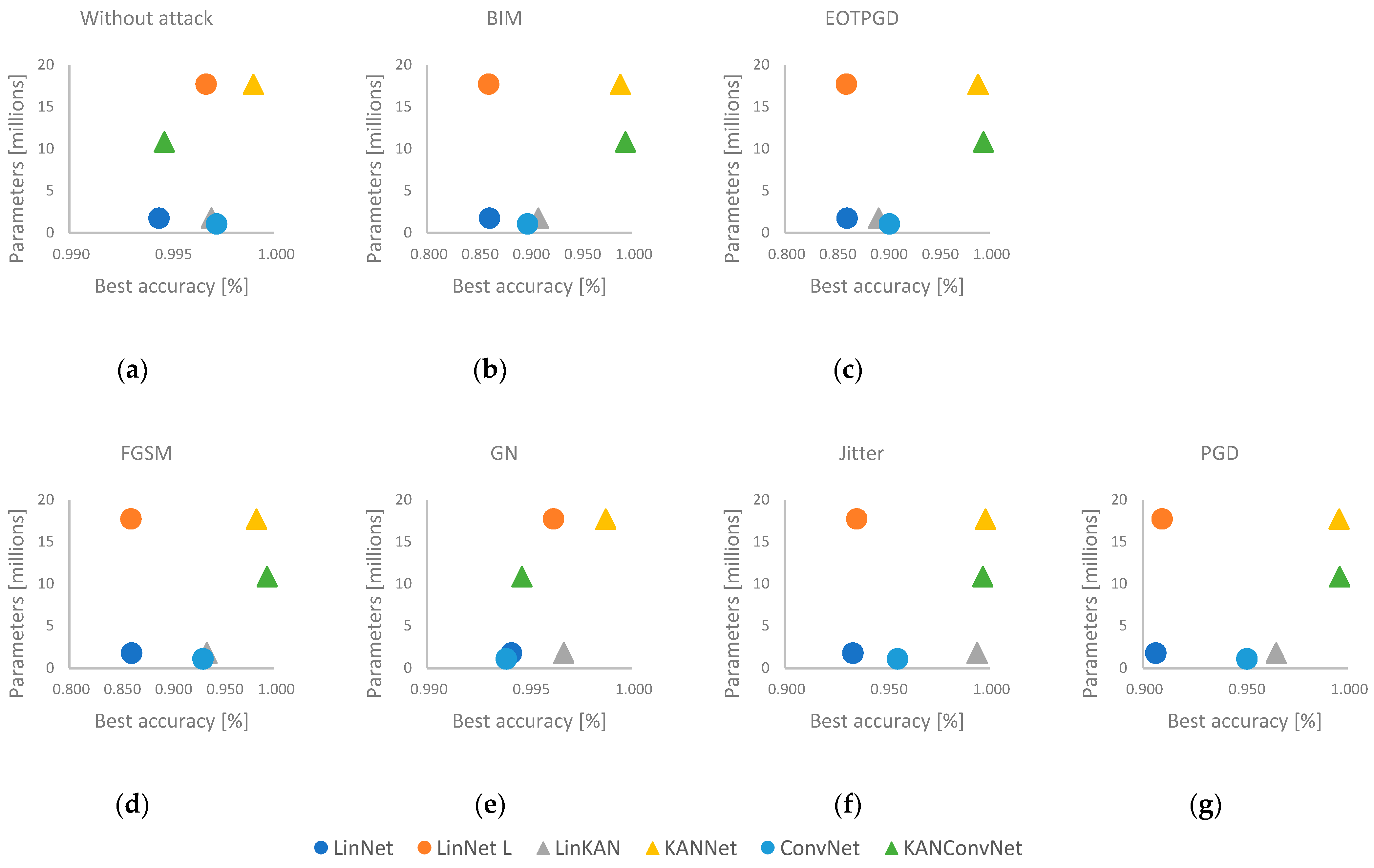
Figure 3 shows the best results and the number of network parameters. The KANNet and LinNet L models have almost the same number of parameters, and their structure is very similar. However, in all cases, the KAN-based solution has achieved better results. It is also worth comparing the LinKAN solution with the ConvNet and LinNet networks. In all cases, the LinKAN solution performs better than the LinNet network, where the architecture of the two methods is very similar. In the case of ConvNet, we are talking about a more complex solution with a similar number of parameters. Here, the LinKAN network performed better than the convolution-based method in five out of the seven cases. In the case of the KANNet and KANConvNet networks, we can see that in five cases, the efficiency of the two solutions is very similar. The exceptions are the no-attack test and the random noise (GN) case. However, the parameter set of KANConvNet is almost half of the parameter set of KANNet. This means that it is worth using the KAN-based solution together with a convolutional layer. In the left diagram of Figure 4, we can see the largest efficiency degradation for each solution compared to the case without attack. On the right side of Figure 4, we can observe how much efficiency degradation each attack method caused for the networks. Here, it can be seen that the degradations for the KANNet and KANConvNet solutions are negligible compared to the other solutions. For LinKAN, which has a much simpler architecture, we also see that it typically performs better compared to MLP-based solutions.

6. Conclusions

This work focused on the practical applicability of a rather new theory of neural networks, called Kolmogorov–Arnold Networks. The aim of the research was to develop a unique dataset for long-term goals. Using this dataset, different network architectures were investigated. A comparison was made between traditional MLP-based solutions and KAN-based solutions. How the effectiveness of a solution varies when different attack methods are used was investigated. As a result of these tests, it is clear that KAN-based solutions are able to compete with MLP. It was shown that in the vast majority of cases, KAN-based solutions can be used with higher reliability, as they are more resistant to different noise-attack techniques. Further studies are needed in the area in the future. One of the objectives is to expand the current dataset. It is also necessary to carry out efficiency measurements in case of further network developments. The KAN theory can be extended to the convolution layer, so an in-depth investigation of this could also be the subject of a future research period.

References

- Liu, Z.; Wang, Y.; Vaidya, S.; Ruehle, F.; Halverson, J.; Soljačić, M.; Hou, T.Y.; Tegmark, M. KAN. Kolmogorov-Arnold Networks. arXiv 2024, arXiv:2404.19756. [Google Scholar]
- Kolmogorov, A.N. On the Representation of Continuous Functions of Several Variables as Superpositions of Continuous Functions of One Variable and Addition. Dokl. Akad. Nauk SSSR 1957, 114, 953–956. [Google Scholar]
- Schmidt-Hieber, J. The Kolmogorov-Arnold Representation Theorem Revisited. arXiv 2020, arXiv:2007.15884v2. [Google Scholar] [CrossRef] [PubMed]
- Rawat, W.; Wang, Z. Deep Convolutional Neural Networks for Image Classification: A Comprehensive Review. Neural Comput. 2017, 29, 2352–2449. [Google Scholar] [CrossRef] [PubMed]
- Garcia-Garcia, A.; Orts-Escolano, S.; Oprea, S.; Villena-Martinez, V.; Martinez-Gonzalez, P.; Garcia-Rodriguez, J. A Survey on Deep Learning Techniques for Image and Video Semantic Segmentation. Appl. Soft Comput. 2018, 70, 41–65. [Google Scholar] [CrossRef]
- Zhao, Z.Q.; Zheng, P.; Xu, S.; Wu, X. Object Detection with Deep Learning: A Review. arXiv 2019, arXiv:1807.05511. [Google Scholar] [CrossRef] [PubMed]
- Sze, V.; Chen, Y.H.; Yang, T.J.; Emer, J. Efficient Processing of Deep Neural Networks: A Tutorial and Survey. arXiv 2017, arXiv:1703.09039. [Google Scholar] [CrossRef]
- Deng, L.; Li, G.; Han, S.; Shi, L.; Xie, Y. Model Compression and Hardware Acceleration for Neural Networks: A Comprehensive Survey. Proc. IEEE 2020, 108, 485–532. [Google Scholar] [CrossRef]
- Vaishnav, M.; Cadene, R.; Alamia, A.; Linsley, D.; VanRullen, R.; Serre, T. Understanding the Computational Demands Underlying Visual Reasoning. Neural Comput. 2022, 34, 1075–1099. [Google Scholar] [CrossRef] [PubMed]
- Hendrycks, D.; Gimpel, K. Gaussian Error Linear Units (GELUs). arXiv 2016, arXiv:1606.08415v5. [Google Scholar]
- Agarap, A.F. Deep Learning Using Rectified Linear Units (ReLU). arXiv 2018, arXiv:1803.08375v2. [Google Scholar]
- Kurakin, A.; Goodfellow, I.; Bengio, S. Adversarial Examples in the Physical World. arXiv 2017, arXiv:1607.02533. [Google Scholar]
- Zimmermann, R.S. Comment on “Adv-BNN: Improved Adversarial Defense through Robust Bayesian Neural Network”. arXiv 2019, arXiv:1907.00895. [Google Scholar]
- Goodfellow, I.J.; Shlens, J.; Szegedy, C. Explaining and Harnessing Adversarial Examples. arXiv 2015, arXiv:1412.6572. [Google Scholar]
- Schwinn, L.; Raab, R.; Nguyen, A.; Zanca, D.; Eskofier, B. Exploring Misclassifications of Robust Neural Networks to Enhance Adversarial Attacks. arXiv 2021, arXiv:2105.10304. [Google Scholar] [CrossRef]
- Madry, A.; Makelov, A.; Schmidt, L.; Tsipras, D.; Vladu, A. Towards Deep Learning Models Resistant to Adversarial Attacks. arXiv 2019, arXiv:1706.06083. [Google Scholar]
- Kim, H. Torchattacks: A PyTorch Repository for Adversarial Attacks. arXiv 2021, arXiv:2010.01950. [Google Scholar]
- Kingma, D.P.; Ba, J. Adam: A Method for Stochastic Optimization. arXiv 2014, arXiv:1412.6980v9. [Google Scholar]
Disclaimer/Publisher’s Note: The statements, opinions and data contained in all publications are solely those of the individual author(s) and contributor(s) and not of MDPI and/or the editor(s). MDPI and/or the editor(s) disclaim responsibility for any injury to people or property resulting from any ideas, methods, instructions or products referred to in the content. |
© 2024 by the author. Licensee MDPI, Basel, Switzerland. This article is an open access article distributed under the terms and conditions of the Creative Commons Attribution (CC BY) license (https://creativecommons.org/licenses/by/4.0/).