Accuracy of NTC Thermistor Measurements Using the Sensor to Microcontroller Direct Interface ^†

Abstract

Portable and wearable sensor systems are usually based on microcontrollers or field programmable gate arrays (FPGAs), where the sensors are measured using an analog-to-digital converter (ADC). An alternative solution, with benefits in terms of cost reduction and lower power consumption, is the sensor-to-microcontroller direct interface (SMDI), a technique where the sensor is measured using the general purpose input output (GPIO) interface present on any microcontroller or FPGA. In this paper, the measurement accuracy of a non-linear temperature sensor (NTC 3950) using SMDI was evaluated by means of LTSpice simulations in the temperature range from −10 °C to 80 °C. The temperature was estimated using two different models and the results have shown that the most accurate model (Steinhart–Hart model) achieves an average temperature error of 0.078 °C.

1. Introduction

The interest in portable and wearable sensor systems is continuously increasing with impact on both research activity and market size. These systems are usually built on the paradigm of the Internet of Things (IoT), where a number of distributed sensor nodes (edge devices) communicate using wireless technologies and transfer data to a main host for data processing and analysis [1]. Portable and wearable sensor systems are adopted for a wide range of applications, such as environmental monitoring [2,3,4], microbial analysis [5,6,7,8], food safety [9,10,11,12], health monitoring [13,14,15,16], and quality analysis in industrial environments [17,18,19]. Edge devices, usually based on microcontrollers or field programmable gate arrays (FPGAs), are interfaced to the sensors using an analog-to-digital converter (ADC), that is used to measure the sensor analog output and convert it to a digital format for data processing and transmission. Edge devices are usually powered by batteries or energy harvesting; thus, their power consumption is critical and can seriously impact the sensor node lifetime [20,21].

At this regard, sensor-to-microcontroller direct interface (SMDI) is a popular technique that allows sensor measurements without an ADC with benefits in terms of cost reduction and lower power consumption [22,23]. In SMDI, the Schmitt trigger integrated in the general purpose input output (GPIO) interface of a microcontroller is exploited as an analog comparator for sensor measurements. This technique has been applied to many types of sensors, such as resistive and capacitive sensors, as well as sensors featuring an analog output voltage. A SMDI application for the measurement of three-wire [24] and four-wire [25] resistive sensors was proposed by Reverter in 2022. Techniques based on SMDI for the measurement of capacitive sensors [26] and lossy capacitive relative humidity sensors [27] were proposed by Czaja in 2020 and 2021. In 2024, Grossi presented a technique based on SMDI for the measurement of an analog voltage without an ADC and implemented it on a low-cost FPGA [28].

In the proposed study, the application of SMDI is investigated in the case of a non-linear negative temperature coefficient (NTC) thermistor using two different models (Steinhart–Hart model and polynomial model) to estimate the temperature from the sensor data. The system was tested under real operative conditions in presence of noise using LTSpice XVII simulations and the two models were compared in terms of accuracy. The results have shown that the temperature estimation using the Steinhart–Hart model provides more accurate results (average error 0.078 °C), in particular in the case of low temperatures, while the polynomial model features an average error of 0.28 °C. In Section 2, the basics of SMDI for the measurement of a resistive sensor are presented. In Section 3, the resistive temperature sensor used in the simulations and the two mathematical models for temperature estimation are presented. In Section 4, the results of the simulations are shown, while in Section 5, conclusive remarks are drawn.

2. Sensor-to-Microcontroller Direct Interface

The schematic of the circuit used to measure the resistance value of the temperature sensor using SMDI is presented in Figure 1. Here, the Schmitt trigger circuit, featuring an hysteresis window with two thresholds V_H and V_L, is integrated in the microcontroller GPIO interface and converts the analog voltage V₁ into a digital signal V_1,dig. The digital output pin (with voltage V₂) is driven by the microcontroller CPU to charge/discharge the capacitance C through the non-linear temperature sensor with resistance R_T.

The circuit behaves like an astable multivibrator. When the analog voltage V₁ increases over V_H, the signal V_1,dig switches from 0 to V_DD. The value of V_1,dig is read by the CPU that drives the output pin to V₂ = 0, and thus discharging the capacitance C. Similarly, when V₁ decreases below V_L, the signal V_1,dig switches from V_DD to 0. The value of V_1,dig is read by the CPU that drives the output pin to V₂ = V_DD, thus charging the capacitance C.

During the charging phase of the capacitance C, the signal V₁ increases from V_L to V_H with V₂ = V_DD. The circuit can be modelled with the following differential equation:

$$C{\displaystyle \frac{d{V}_1}{dt}}={\displaystyle \frac{V_{DD}-V_1}{R_T}}$$

(1)

Indicating with t_H the rising time of signal V₁, this value can be calculated by integrating the differential Equation (1).

$$t_H=R_{T}C\underset{V_L}{\overset{V_H}{\int }}{\displaystyle \frac{1}{V_{DD}-V_1}}d{V}_1=R_{T}C·log{\displaystyle \frac{V_{DD}-V_L}{V_{DD}-V_H}}$$

(2)

During the discharging phase of the capacitance C, instead, the signal V₁ decreases from V_H to V_L with V₂ =0. The circuit can be modelled with the following differential equation:

$$C{\displaystyle \frac{d{V}_1}{dt}}=-{\displaystyle \frac{V_1}{R_T}}$$

(3)

Indicating with t_L the falling time of signal V₁, this value can be calculated by integrating the differential Equation (3), as follows:

$$t_L=-R_{T}C\underset{V_H}{\overset{V_L}{\int }}{\displaystyle \frac{1}{V_1}}d{V}_1=R_{T}C·log{\displaystyle \frac{V_H}{V_L}}$$

(4)

The period T_P of the signals V₁ and V₂ can thus be calculated as follows:

$$T_P=t_H+t_L=R_{T}C·log{\displaystyle \frac{V_H\left(V_{DD}-V_L\right)}{V_L\left(V_{DD}-V_H\right)}}$$

(5)

The period T_P can be measured with a digital timer integrated in the microcontroller. Considering a case study of a 16-bit timer with a clock frequency f_CLK = 64 MHz (clock period T_CLK = 15.625 ns), it is T_P = N·T_CLK, where N is the digital counter value. Thus, the resistance value of the temperature sensor can be calculated as follows:

$$R_T={\displaystyle \frac{N{T}_{CLK}}{C·log\frac{V_H\left(V_{DD}-V_L\right)}{V_L\left(V_{DD}-V_H\right)}}}$$

(6)

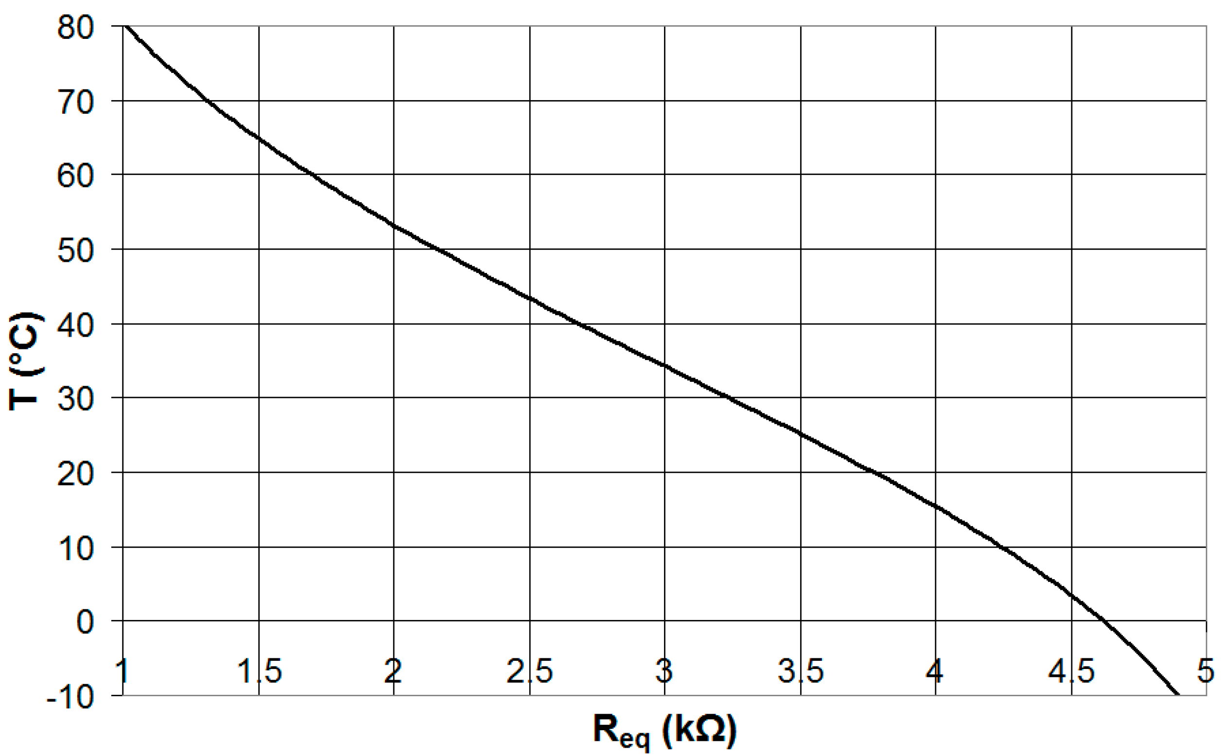
3. The NTC Temperature Sensor

Negative temperature coefficient (NTC) temperature sensors are non-linear resistors, whose resistance value changes with temperature. The resistance of NTC sensors decreases as the temperature increases. The characteristic of an NTC 3950 temperature sensor (Conrad Electronic, Hirschau, Germany) [29] is presented in Figure 2 in the case of the temperature range −10–80 °C.

As can be seen, the characteristic of the NTC 3950 sensor is strongly non-linear and its sensitivity, i.e., the resistance variation for temperature variations of 1 °C is higher for low temperatures.

The non-linear function that best fits the characteristic of an NTC temperature sensor is the Steinhart–Hart model, as follows:

$$T={\displaystyle \frac{1}{k_1+k_{2}log{R}_T+k_3{\left(log{R}_T\right)}^3}}-273.15$$

(7)

where T is the temperature expressed in °C; R_T is the temperature sensor resistance expressed in kΩ; and k₁, k₂, k₃ are the parameters used to fit the model with the experimental data. The model defined by Equation (7) provides a good fit to the experimental data values of an NTC temperature sensor. However, the model is computationally intensive and the achieved accuracy depends on the temperature value.

A technique used to improve the linearity of the thermistor characteristic is to put a fixed resistance R_P in parallel to the NTC temperature sensor. The equivalent resistance R_eq = R_T || R_P has been calculated for a set of R_P values (from 100 Ω to 100 kΩ) and R_T values obtained from the thermistor characteristic for temperature values in the range from −10 °C to 80 °C. The characteristic of temperature as function of R_eq was fitted to a linear regression line and the mean squared error (MSE) resulting from the temperature estimation using the regression line was calculated for each value of R_P. The results are presented in Figure 3.

The value of R_P that maximizes the linearity between the temperature and R_eq (i.e., it achieves the minimum MSE) is 5.41 kΩ. The characteristic of the temperature as a function of the resistance R_eq is presented in Figure 4, in the case of R_P = 5.41 kΩ.

The characteristic shown in Figure 4 can be modelled using a polynomial equation of order 3, as follows:

$$T=h_1+h_2{R}_{eq}+h_3{R}_{eq}^2+h_4{R}_{eq}^3$$

(8)

where T is the temperature expressed in °C; R_eq = R_T || R_P is expressed in kΩ; and h₁, h₂, h₃, h₄ are parameters used to fit the model with the experimental data.

The models defined by Equations (7) and (8) were fitted to the temperature sensor characteristic obtained from its data sheet and the error in the estimated temperature (|ΔT|) calculated and plotted vs. the environmental temperature T for both models. The results are presented in Figure 5. As can be seen, the Steinhart–Hart model provides higher accuracy than the polynomial model with a maximum error in the estimated temperature that is always below 0.1 °C.

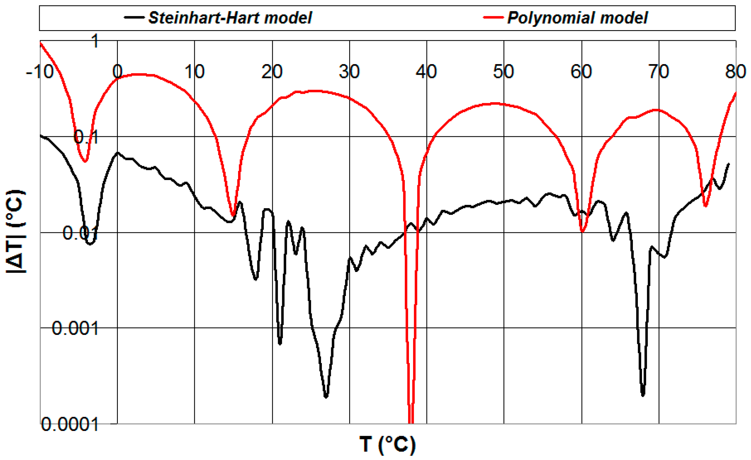
4. Simulation Results

The circuit of Figure 1 was simulated using LTSpice [30] for the following two cases: (a) the NTC temperature sensor R_T is connected between nodes 1 and 2 with C = 33 nF; (b) the parallel of the NTC temperature sensor R_T and a fixed resistor R_P of value 5.41 kΩ is connected between nodes 1 and 2 with C = 330 nF. In the case (a), the temperature was estimated using the Steinhart–Hart model, while in the case (b), the temperature was estimated using the polynomial model. The thresholds of the Schmitt trigger integrated in the microcontroller GPIO interface were set to V_L = 1.196 V V_H = 1.644 V as a case study, since these are the threshold values of the Schmitt trigger circuit integrated in the GPIO interface of the low-cost microcontroller STM32L073RZT6 (ST Microelectronics) [31]. The period of the square-wave signal V₂ (T_P) was measured using a 16-bit counter with a clock frequency of 64 MHz (clock period T_CLK = 15.625 ns) and a white noise voltage of peak values ±50 mV was superimposed to node 1 to simulate a real measurement scenario. The case of ten different environmental temperatures between −10 °C and 80 °C was considered and, for each temperature, 20 simulations were carried out. For each temperature, the average estimated temperature (T_est) for the 20 simulations, the error in the average estimated temperature (|ΔT_error|), the standard deviation (σ_T), and the maximum (T_max) and minimum (T_min) values of the estimated temperature were calculated. The simulation results are reported in

Table 1. Simulation results for the case of the NTC temperature sensor between nodes 1 and 2. The temperature is estimated with the Steinhart–Hart model.

T (°C)	Test (°C)	|ΔTerror| (°C)	σT (°C)	Tmax (°C)	Tmin (°C)
−10	−9.843	0.157	0.107	−9.643	−9.986
0	−0.094	0.094	0.103	0.109	−0.325
10	9.858	0.141	0.207	10.276	9.569
20	19.942	0.058	0.195	20.197	19.638
30	30.022	0.022	0.172	30.443	29.691
40	40.091	0.091	0.258	40.545	39.711
50	50.061	0.061	0.352	50.586	49.360
60	59.999	0.001	0.316	60.771	59.293
70	70.066	0.066	0.367	70.667	69.216
80	79.911	0.089	0.440	80.637	79.131

for the case (a), and in

Table 2. Simulation results for the case of the parallel of the NTC temperature sensor and a fixed resistor of value 5.41 kΩ between nodes 1 and 2. The temperature is estimated with the polynomial model.

T (°C)	Test (°C)	|ΔTerror| (°C)	σT (°C)	Tmax (°C)	Tmin (°C)
−10	−9.571	0.428	1.013	−7.982	−11.975
0	−0.463	0.463	0.644	0.589	−1.665
10	9.581	0.419	0.703	10.677	8.489
20	20.367	0.367	0.404	20.890	19.499
30	30.309	0.309	0.273	30.645	29.699
40	40.017	0.017	0.264	40.376	39.575
50	49.684	0.316	0.273	50.160	49.123
60	59.861	0.139	0.286	60.346	59.362
70	70.291	0.291	0.398	70.931	69.209
80	79.930	0.070	0.379	80.637	79.311

for the case (b). The results show that the temperature estimation using the Steinhart–Hart model provides more accurate results, in particular in the case of low temperatures (average error 0.078 °C in the temperature range from −10 °C to 80 °C), while the polynomial model features an average error of 0.28 °C.

5. Conclusions

In this paper, the measurement accuracy of a non-linear resistive temperature sensor (NTC 3950) was investigated using the sensor-to-microcontroller direct interface, a popular technique for sensor measurements without an analog-to-digital converter. The sensor and the measurement system were simulated by means of the circuital simulator LTSpice and the temperature was estimated using two different models, the Steinhart–Hart model and the polynomial model.

The results have shown how the Steinhart–Hart model features higher accuracy, with an average error of 0.078 °C on the temperature range from −10 °C to 80 °C, while the polynomial model is less computationally intensive than the Steinhart–Hart model, but features a lower accuracy (average error of 0.28 °C).

References

1. Laghari, A.A.; Wu, K.; Laghari, R.A.; Ali, M.; Khan, A.A. A review and state of art of Internet of Things (IoT). Arch. Comput. Methods Eng. 2021, 29, 1395–1413. [Google Scholar] [CrossRef]
2. Ziętek, B.; Banasiewicz, A.; Zimroz, R.; Szrek, J.; Gola, S. A portable environmental data-monitoring system for air hazard evaluation in deep underground mines. Energies 2020, 13, 6331. [Google Scholar] [CrossRef]
3. Sgobba, F.; Sampaolo, A.; Patimisco, P.; Giglio, M.; Menduni, G.; Ranieri, A.C.; Hoelzl, C.; Rossmadl, H.; Brehm, C.; Mackowiak, V.; et al. Compact and portable quartz-enhanced photoacoustic spectroscopy sensor for carbon monoxide environmental monitoring in urban areas. Photoacoustics 2022, 25, 100318. [Google Scholar] [CrossRef]
4. Ouni, R.; Saleem, K. Framework for sustainable wireless sensor network based environmental monitoring. Sustainability 2022, 14, 8356. [Google Scholar] [CrossRef]
5. Grossi, M.; Parolin, C.; Vitali, B.; Riccò, B. A portable sensor system for bacterial concentration monitoring in metalworking fluids. J. Sens. Sens. Syst. 2018, 7, 349–357. [Google Scholar] [CrossRef]
6. Grossi, M.; Parolin, C.; Vitali, B.; Riccò, B. Computer vision approach for the determination of microbial concentration and growth kinetics using a low cost sensor system. Sensors 2019, 19, 5367. [Google Scholar] [CrossRef] [PubMed]
7. Pham, H.L.; Ling, H.; Chang, M.W. Design and fabrication of field-deployable microbial biosensing devices. Curr. Opin. Biotechnol. 2022, 76, 102731. [Google Scholar] [CrossRef]
8. Grossi, M.; Parolin, C.; Vitali, B.; Riccò, B. Measurement of bacterial concentration using a portable sensor system with a combined electrical-optical approach. IEEE Sens. J. 2019, 19, 10693–10700. [Google Scholar] [CrossRef]
9. Grossi, M.; Valli, E.; Bendini, A.; Gallina Toschi, T.; Riccò, B. A Portable Battery-Operated Sensor System for Simple and Rapid Assessment of Virgin Olive Oil Quality Grade. Chemosensors 2022, 10, 102. [Google Scholar] [CrossRef]
10. Shen, Y.; Wei, Y.; Zhu, C.; Cao, J.; Han, D.M. Ratiometric fluorescent signals-driven smartphone-based portable sensors for onsite visual detection of food contaminants. Coord. Chem. Rev. 2022, 458, 214442. [Google Scholar] [CrossRef]
11. Xu, J.; Wang, J.; Li, Y.; Zhang, L.; Bi, N.; Gou, J.; Zhao, T.; Jia, L. A wearable gloved sensor based on fluorescent Ag nanoparticles and europium complexes for visualized assessment of tetracycline in food samples. Food Chem. 2023, 424, 136376. [Google Scholar] [CrossRef]
12. Grossi, M.; Bendini, A.; Valli, E.; Gallina Toschi, T. Field-Deployable Determinations of Peroxide Index and Total Phenolic Content in Olive Oil Using a Promising Portable Sensor System. Sensors 2023, 23, 5002. [Google Scholar] [CrossRef] [PubMed]
13. Siam, A.I.; El-Affendi, M.A.; Abou Elazm, A.; El-Banby, G.M.; El-Bahnasawy, N.A.; Abd El-Samie, F.E.; Abd El-Latif, A.A. Portable and real-time IoT-based healthcare monitoring system for daily medical applications. IEEE Trans. Comput. Soc. Syst. 2023, 10, 1629–1641. [Google Scholar] [CrossRef]
14. Wu, T.; Wu, F.; Qiu, C.; Redouté, J.M.; Yuce, M.R. A rigid-flex wearable health monitoring sensor patch for IoT-connected healthcare applications. IEEE Internet Things J. 2020, 7, 6932–6945. [Google Scholar] [CrossRef]
15. Chen, S.; Qi, J.; Fan, S.; Qiao, Z.; Yeo, J.C.; Lim, C.T. Flexible wearable sensors for cardiovascular health monitoring. Adv. Healthc. Mater. 2021, 10, 2100116. [Google Scholar] [CrossRef] [PubMed]
16. Kaur, B.; Kumar, S.; Kaushik, B.K. Novel wearable optical sensors for vital health monitoring systems—A review. Biosensors 2023, 13, 181. [Google Scholar] [CrossRef] [PubMed]
17. Grossi, M.; Riccò, B. A portable electronic system for in-situ measurements of oil concentration in MetalWorking fluids. Sens. Actuators A Phys. 2016, 243, 7–14. [Google Scholar] [CrossRef]
18. Aponte-Luis, J.; Gómez-Galán, J.A.; Gómez-Bravo, F.; Sánchez-Raya, M.; Alcina-Espigado, J.; Teixido-Rovira, P.M. An efficient wireless sensor network for industrial monitoring and control. Sensors 2018, 18, 182. [Google Scholar] [CrossRef]
19. Kalsoom, T.; Ramzan, N.; Ahmed, S.; Ur-Rehman, M. Advances in sensor technologies in the era of smart factory and industry 4.0. Sensors 2020, 20, 6783. [Google Scholar] [CrossRef] [PubMed]
20. Elahi, H.; Munir, K.; Eugeni, M.; Atek, S.; Gaudenzi, P. Energy harvesting towards self-powered IoT devices. Energies 2020, 13, 5528. [Google Scholar] [CrossRef]
21. Callebaut, G.; Leenders, G.; Van Mulders, J.; Ottoy, G.; De Strycker, L.; Van der Perre, L. The art of designing remote iot devices—Technologies and strategies for a long battery life. Sensors 2021, 21, 913. [Google Scholar] [CrossRef] [PubMed]
22. Reverter, F. The art of directly interfacing sensors to microcontrollers. J. Low Power Electron. Appl. 2012, 2, 265–281. [Google Scholar] [CrossRef]
23. Bengtsson, L.E. Analysis of direct sensor-to-embedded systems interfacing: A comparison of targets’ performance. Int. J. Intell. Mechatron. Robot. (IJIMR) 2012, 2, 41–56. [Google Scholar] [CrossRef]
24. Reverter, F. A microcontroller-based interface circuit for three-wire connected resistive sensors. IEEE Trans. Instrum. Meas. 2022, 71, 2006704. [Google Scholar] [CrossRef]
25. Reverter, F. A direct approach for interfacing four-wire resistive sensors to microcontrollers. Meas. Sci. Technol. 2022, 34, 037001. [Google Scholar] [CrossRef]
26. Czaja, Z. A measurement method for capacitive sensors based on a versatile direct sensor-to-microcontroller interface circuit. Measurement 2020, 155, 107547. [Google Scholar] [CrossRef]
27. Czaja, Z. A measurement method for lossy capacitive relative humidity sensors based on a direct sensor-to-microcontroller interface circuit. Measurement 2021, 170, 108702. [Google Scholar] [CrossRef]
28. Grossi, M. Efficient and Accurate Analog Voltage Measurement Using a Direct Sensor-to-Digital Port Interface for Microcontrollers and Field-Programmable Gate Arrays. Sensors 2024, 24, 873. [Google Scholar] [CrossRef] [PubMed]
29. NTC Temperature Sensor 3950 Data Sheet. Available online: https://cdn-shop.adafruit.com/datasheets/103_3950_lookuptable.pdf (accessed on 19 May 2024).
30. LTSpice Circuit Simulator. Available online: https://www.analog.com/en/resources/design-tools-and-calculators/ltspice-simulator.html (accessed on 19 May 2024).
31. STM32L073RZT6 Microcontroller. Available online: https://www.st.com/en/microcontrollers-microprocessors/stm32l073rz.html (accessed on 19 May 2024).
Figure 1. Schematic of the circuit to measure the value of a resistance without an ADC.
Engproc 82 00012 g001
Figure 2. Characteristic of an NTC 3950 temperature sensor.
Engproc 82 00012 g002
Figure 3. Mean squared error resulting from the temperature estimation using the regression line plotted vs. the resistance RP.
Engproc 82 00012 g003
Figure 4. Characteristic of the environmental temperature as function of the resistance Req.
Engproc 82 00012 g004
Figure 5. Error in the estimated temperature achieved using the Steinhart–Hart model and the polynomial model plotted vs. the environmental temperature.
Engproc 82 00012 g005