Predicting Hit Songs Using Audio and Visual Features ^†

Abstract

Factors contributing to a song’s popularity are explored in this study. Recent studies have mainly focused on using acoustic features to identify popular songs. However, we combined audio and visual data to make predictions on 1000 YouTube songs. In total, 1000 songs were grouped into two categories based on YouTube view counts: popular and non-popular. The visual features were extracted using OpenCV. These features were applied using machine learning algorithms, including random forest, support vector machines, decision trees, K-nearest neural networks, and logistic regression. Random forest performed the best, with an accuracy of 82%. Average accuracy increased by 9% in all models when using audio and visual features together. This indicates that visual elements are beneficial for identifying hit songs.

1. Introduction

In the traditional music industry, sales of record labels are the most direct route to financial success. Producers and singers aim to sell as many albums as possible. As the Internet is used widely, music streaming sites have become popular by offering songs for free. People can enjoy music without having to buy an album. Singers put their music online and websites pay them royalties for streams and downloads. Today, the main goal for singers and producers is to make songs that attract listeners. Figuring out what makes a song a hit is valuable in many areas. A song’s popularity is determined by what listeners like, how catchy it is, and its commercial appeal.

Recent studies focus on extracting music audio with machine learning, such as decision trees, support vector machines (SVM)-based models, and logistic regression. In 2015, Anjana used Librosa to extract songs’ audio waveforms to predict the song’s popularity with the XGBoost classification algorithm. The second coefficient of Linear Predictive Coding has an accuracy of 71% [1]. In Mafas’s study, audio features were combined with social media to predict a song’s popularity. As a result, social media features are used to predict these factors with an accuracy increase of up to 10% [2]. In addition to audio features, visual features are an important element in predicting popularity. For instance, Elham used metadata, audio, and visual features to develop a movie recommender system [3].

In previous research, audio features of a song are used to train and predict a song’s popularity with machine learning. However, no-one has studied the relationship between music videos and a song’s popularity. Given that YouTube is an online platform, over half of people aged 13–36 listen to music on it. Therefore, a high-quality music video is the main factor for hit songs.

Using new methods, we predicted a song’s popularity by extracting music video features from YouTube and combining them with an existing dataset that contains audio features. Datasets “Spotify and YouTube” from Kaggle were analyzed using OpenCV to extract the features of the music videos. Then, the dataset combined with audio and visual features was used to predict a song’s popularity using machine learning techniques. Then, we explored which machine learning methods performed best for the proposed model and which visual elements enhanced the prediction of hit songs, and we provide suggestions to the music industry based on these results.

2. Literature Review

2.1. Music Popularity Prediction

Machine learning techniques have been used in various domains for prediction, especially in estimating the popularity of songs. Many researchers use different techniques to create a distinct prediction model. Ogihara highlighted the use of computational methods for genre classification. The introduction of Daubechies Wavelet Coefficient Histograms (DWCHs) is regarded as a significant development. Compared with existing techniques with algorithms such as SVMs and linear discriminant analysis, DWCHs have enhanced the accuracy of music genre classification [4].

Building on the computational approach, Dhanaraj and Logan predicted hit songs using automatic music analysis. They used a database containing 1700 songs with acoustic and lyric information to classify tracks as hits or non-hits using SVMs and boosting classifiers. They concluded that lyric-based features are more effective than acoustic features in identifying potential hits. However, the methods are not successful, with much room for improvement [5]. Borg and Hokkanen explored the relationship between acoustic features, genre, and YouTube view counts to predict hit songs. Their data were obtained from the Million Song Dataset with 10,000 songs and its pre-extracted features. By combining SVM and K-means clustering, an accuracy of 55% was achieved. The artist’s popularity was found to be correlated with hit songs, regardless of the acoustic features [6]. Yang and Hu predicted the popularity of non-Western songs (Chinese songs in this case) using Western songs’ mood classification models. They classified audio features for Western and Chinese music and compared the performance of mood classification. They considered psychoacoustic features to apply to Chinese songs with an accuracy of 74.7% [7].

As a modern technique, Yang et al. focused on using deep learning algorithms such as the convolutional neural network (CNN) model and the JYnet model to enhance the prediction of hit songs. The dataset was obtained from KKBOX with information about Taiwanese users’ listening records from 2012 to 2013. The data were used to train shallow and deep learning models by framing it as a regression problem. Deep learning models performed better and highlighted the importance of how genres are proportioned in the learning algorithms [8].

In various studies, various data features with machine learning algorithms are used to predict hit songs. Rajyashree et al. used MIDI features [9], Yang et al. used high and low levels of audio features [10], Pham et al. combined songs with information such as artist names [11], Kim and Oh used granular acoustic features [12], and Nikas et al. used datasets of audio features, lyrics, and temporal features [13]. Mayerl et al. introduced ordinal classification to predict hit songs. They utilized two datasets containing 7736 and 73,432 songs to test classification, regression, and ordinal models. They suggested that ordinal classification has similar accuracy to classification and regression models and, in some cases, performed better [14].

These studies used machine learning to predict song popularity with various features such as acoustic properties, lyrics, and genre classifications. However, the primary focus was put on audio features to predict hits. Based on previous results, we incorporated visual features into audio features to enhance the predictive accuracy of hit songs.

2.2. Sound

Sound is characterized by several fundamental parameters essential for understanding its manipulation in various applications. The first one is frequency, which determines the pitch of a sound, and this is measured in Hertz (Hz). The second one is amplitude, indicating the volume or loudness of a sound, and this is measured in decibels (db). Waveform is measured by both frequency and amplitude, giving the shape of the sound wave [15]. Waveform represents sound in time and frequency domains. The time domain represents how the sound signal changes over time. Conversely, the frequency domain represents the breakdown of sound into its frequencies, each with its amplitude. Fourier Transform is used in the frequency domain by breaking down signals into the sum of sinusoidal functions. Sound can be captured using multiple digital formats, including WAV, MP3, AAC, and FLAC [16].

2.3. Visual Elements

Chang et al. introduced license plate recognition (LPR) with minimal environmental constraints. Using a dataset of 1088 images, they applied modules with color edge detectors to identify the image and number on the plate. The color detector’s accuracy reached 93.7% [17]. Expanding the application of visual elements, Devi et al. used an image processing system to predict fruit yield based on its color and shape. Images of the fruit trees were taken and processed by OpenCV using an image processing algorithm. Machine learning algorithms achieved 94% accuracy [18]. Visual elements in agriculture are used in plant disease detection. Domingues used the online dataset PlantVillage with 18,160 images of tomatoes to extract features such as color distributions and texture patterns. SVM, Random Forest (RF), and Artificial Neural Networks (ANNs) were trained, achieving an accuracy above 90% in predicting tomato diseases [19]. Nageswaran et al. used image processing techniques such as noise reduction and feature extraction with the K-means technique to classify and predict lung cancer. They used a dataset of 83 CT scans from 70 patients. For this task, classification was performed using ANN, KNN, and RF. The ANN model showed the highest accuracy in predicting lung cancer.

Previous studies indicated that visual elements can be used for prediction with machine learning. They are not used to predict hit songs yet.

3. Materials and Methods

Figure 1 shows a flow chart of this research. Data were gathered from ‘Spotify and YouTube’ from 7 February 2023, including 20,717 songs on YouTube. The dataset was obtained from Kaggle. In total, 18 features were extracted, including 11 audio features and song information such as song title, artist, view count, etc. Data were collected from 13 April to 21 May 2023. After cleaning the dataset, 5 visual features were extracted using OpenCV and merged with audio features into a new dataset. The highest and lowest 500 songs in terms of YouTube views were labeled as popular and unpopular categories. Classification machine learning was used for audio and visual features.

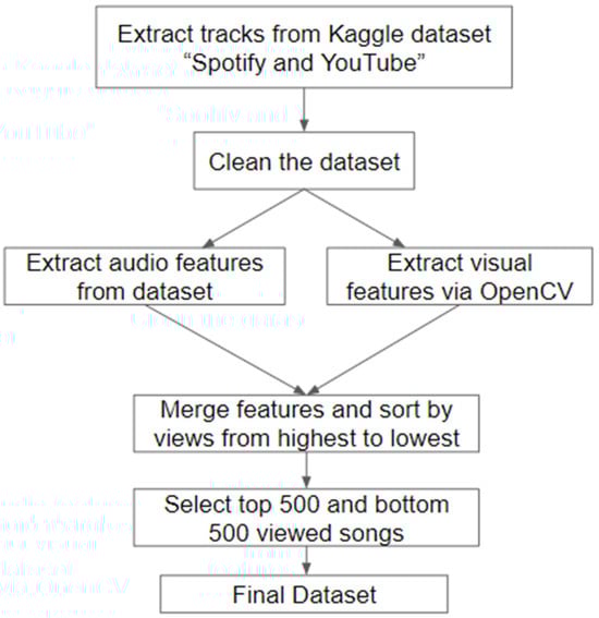
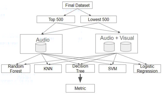
Figure 2 shows the structure of this research. Two experiments were conducted to showcase the significance of visual features in prediction. The first dataset contained audio features. In total, 5 distinct machine learning models were used. The second dataset containing audio and visual features was processed with the same machine learning models.

3.1. Independent Variables

The 10 sets of audio features were determined from the dataset. A description of the features is shown in

Table 1. Audio features.

Features	Description
Danceability	Describes how suitable a track is for dancing based on a combination of musical elements. A value of 0.0 is least danceable and 1.0 is the most danceable.
Energy	A measure from 0.0 to 1.0 which represents a perceptual measure of intensity and activity.
Key	The key the track is in. Integers map to pitches using standard Pitch Class notation.
Loudness	The overall loudness of a track in decibels (dB).
Speechiness	The presence of spoken words in a track. The more exclusively speech-like the recording (e.g., talk show, audio book, poetry), the closer to 1.0 the attribute value.
Acousticness	A confidence measure from 0.0 to 1.0 of whether the track is acoustic: 1.0 represents high confidence that the track is acoustic.
Liveness	The presence of an audience in the recording. Higher liveness values represent an increased probability that the track was performed live.
Valence	A measure from 0.0 to 1.0 describing the musical positiveness conveyed by a track. Tracks with high valence sound more positive (e.g., happy, cheerful, euphoric), while tracks with low valence sound more negative (e.g., sad, depressed, angry).
Tempo	The overall estimated tempo of a track in beats per minute (BPM).
Duration_ms	The duration of the track in milliseconds.

.

In total, 5 sets of visual features were acquired from OpenCV using the dataset YouTube playlist. The description of the features can be shown in

Table 2. YouTube visual features.

Features	Description
Average brightness	The average luminance level across all frames of a video.
Average motion	The average magnitude of change between consecutive frames.
Average R value	The mean intensity of the red color across all pixels in a video.
Average G value	The mean intensity of the green color across all pixels in a video.
Average B value	The mean intensity of the blue color across all pixels in a video.

.

3.2. Dependent Variables

In total, 20,717 songs and 2079 artists were contained in the dataset. After eliminating invalid audio files and missing values, 18,774 songs remained. The top 500 highest-view-count videos were combined with the 500 lowest-view-count videos to create the final dataset. Cross-validation with 5 folds was performed on this dataset. Accuracy and F1-score were calculated for evaluating binary classifiers.

4. Results

Five different machine learning models were used to explore the effect of visual elements on hit song prediction, and the visual element correlation between popular and non-popular songs was analyzed.

4.1. Accuracy of Models

Table 3. Comparisons of average accuracy and F1-score of the five algorithms with audio and visual elements.

Algorithm	Audio Accuracy	Audio+Visual Accuracy	Audio F1-Score	Audio+Visual F1-Score
Support Vector Machine	72.57%	80.68%	71.98%	80.57%
Random Forest	73.87%	81.98%	73.57%	80.57%
Decision Tree	69.26%	76.47%	69.06%	76.40%
KNN	63.37%	74.77%	62.84%	74.29%
Logistic Regression	72.57%	80.78%	72.10%	80.69%
Average	70.33%	78.93%	69.91%	78.76%

summarizes the comparison results for the five models. The best-performing model is highlighted for each column. Out of the five models, RF exceeded the others by all four metrics. It outperformed in both audio features and audio combined with visual features, showing higher accuracy and F1-score. On the other hand, KNN had the poorest results across all metrics compared to the rest. There was an increase in accuracy after including visual features. Every model had an improvement ranging from 7 to 12%.

4.2. Visual Features

Table 4. Comparisons of average value of five visual elements with audio and visual elements.

Features	Non-Popular Songs	Popular Songs
Average R Value	43   91   141	42   73   104
	#2B0000 #5B0000 #8D0000	#2A0000 #490000 #680000
Average G Value	35   82   130	39   67   95
	#002300 #005200 #008200	#002700 #004300 #005F00
Average B Value	32   80   128	36   65   94
	#000020 #000050 #000080	#000024 #000041 #00005E
Average	(91,82,80)	(73,67,65)

reveals significant differences in multiple characteristics. The t-test results indicate that all five features showed marked differences between the two groups from the low p-values. Table 4 also shows the difference in mean values for five visual features between popular and non-popular songs. Out of the five visual features, non-popular songs showed higher brightness and color values. However, popular songs had significantly higher motion values with an average of 7.78 compared to 3.18 in non-popular songs.

The following hypotheses were proposed and tested to determine significant differences in terms of brightness, motion, and RGB values. The first hypothesis (H1) suggested that the average brightness of non-popular songs is equal to the average brightness of popular songs.

• Hypothesis 1:

• H₀: The average brightness of non-popular songs is equal to the average brightness of popular songs.
• $\left({average brightness \mathrm{\mu }}_{non\text{-}popular}={average brightness \mathrm{\mu }}_{popular}\right)$
• H₁: The average brightness of non-popular songs is not equal to the average brightness of popular songs.
• $\left({average brightness \mathrm{\mu }}_{non\text{-}popular}\ne {average brightness \mathrm{\mu }}_{popular}\right)$

The average brightness for non-popular songs was 85.04, while for popular songs it was 68.93. The p-value was less than 0.05, which shows that the average brightness for popular songs was significantly lower than that of non-popular songs.

The second hypothesis (H2) suggested that the average motion of non-popular songs is equal to the average motion of popular songs.

• Hypothesis 2:

• H₀: The average motion of non-popular songs is equal to the average motion of popular songs.
• $\left({average motion \mathrm{\mu }}_{non\text{-}popular}={average motion \mathrm{\mu }}_{popular}\right)$
• H₁: The average motion of non-popular songs is not equal to the average motion of popular songs.
• $\left({averager motion \mathrm{\mu }}_{non\text{-}popular}\ne {average motion \mathrm{\mu }}_{popular}\right)$

The average motion for non-popular songs was 3.18, while for popular songs it was 7.78. The p-value of 8.10 × 10⁻⁶⁴ was less than 0.05, which showed that the average motion for popular songs was significantly higher than that of non-popular songs.

The third hypothesis (H3) suggested that the average R value of non-popular songs was equal to that of popular songs.

• Hypothesis 3:

• H₀: The average R value of non-popular songs is equal to the average R value of popular songs.
• $\left({average Rvalue\mathrm{\mu }}_{non\text{-}popular}={average Rvalue\mathrm{\mu }}_{popular}\right)$
• H₁: The average R value of non-popular songs is not equal to the average R value of popular songs.
• $\left({averager Rvalue\mathrm{\mu }}_{non\text{-}popular}\ne {average Rvalue\mathrm{\mu }}_{popular}\right)$

The average R value for non-popular songs was 91.82, while for popular songs it was 73.81. The p-value was less than 0.05, which showed that the average R value for popular songs was significantly lower than that of non-popular songs.

The fourth hypothesis (H4) suggested that the average G value of non-popular songs was equal to the average G value of popular songs.

• Hypothesis 4:

• H₀: The average G value of non-popular songs is equal to the average G value of popular songs.
• $\left({average Gvalue\mathrm{\mu }}_{non\text{-}popular}={average Gvalue\mathrm{\mu }}_{popular}\right)$
• H₁: The average G value of non-popular songs is not equal to the average G value of popular songs.
• $\left({averager G-value\mathrm{\mu }}_{non\text{-}popular}\ne {average Gvalue\mathrm{\mu }}_{popular}\right)$

The average G value for non-popular songs was 82.53, while for popular songs it was 67.08. The p-value was less than 0.05, which showed that the average G value for popular songs was significantly lower than that of non-popular songs.

The fifth hypothesis (H5) suggested that the average B value of non-popular songs is equal to the average B value of popular songs.

• Hypothesis 5:

• H₀: The average B value of non-popular songs is equal to the average B value of popular songs.
• $\left({average Bvalue\mathrm{\mu }}_{non\text{-}popular}={average Bvalue\mathrm{\mu }}_{popular}\right)$
• H₁: The average B value of non-popular songs is not equal to the average B value of popular songs.
• $\left({averager Bvalue\mathrm{\mu }}_{non\text{-}popular}\ne {average Bvalue\mathrm{\mu }}_{popular}\right)$

The average B value for non-popular songs was 80.37, while for popular songs it was 65.88. The p-value was less than 0.05, which showed that the average B value for popular songs was significantly lower than that of non-popular songs.

There were significant differences in RGB values between non-popular and popular songs. Interestingly, popular songs had lower RGB values than non-popular songs, considering the mean and standard deviation. For popular songs, the average R-value (73, #490000) was substantially lower than that for non-popular songs (91, #5B0000), similar to the upper bound (104, #680000 vs. 141, #8D0000) and lower bound (42, #2A0000 vs. 43, #2B0000), which refers to the mean R-value. Popular songs had higher intensity and saturation in their color elements. The mean and standard deviation values confirmed that these differences were statistically significant, which implied that brightness and color were influential factors in a song’s popularity.

When inspecting the lower and upper values for popular and non-popular songs, popular songs showed a smaller difference between the bonds, while non-popular songs had a larger one. Popular songs showed colors within a narrower range, while non-popular songs had more diverse visual presentations.

5. Conclusions

Using acoustic and visual elements, we predicted the song’s popularity. RF was the top-performing algorithm for predicting music popularity for all four metrics, with an accuracy of 81.98% and an F1-score of 81.85%. Visual elements in YouTube videos are beneficial for the overall prediction of hit songs, increasing accuracy by 81.85% and F1-score by 8.28%. The t-test results show that popular songs had higher motion compared to non-popular songs. Movement in a song’s music video is crucial, indicating that dances and background changes are important in creating a hit song. Conversely, popular songs had lower RGB and brightness values than non-popular songs, indicating darker, dimmer colors. Additionally, popular songs showed a more consistent color in a narrower range, whereas non-popular songs showed diverse colors.

The dataset was uploaded in 2023. Thus, view counts may vary. In addition, songs are added or removed frequently to maintain an up-to-date dataset for further analysis. We used five visual features. Further research is necessary to extract more visual elements such as thumbnail quality, visual effects, or dance choreography. Additionally, the genres of the song needs to be added to predict its popularity.

References

- Anjana, S. A Robust Approach to Predict the Popularity of Songs by Identifying Appropriate Properties. Ph.D. Thesis, University of Colombo School of Computing, Colombo, Sri Lanka, 2021. [Google Scholar]
- Yee, Y.K.; Raheem, M. Predicting music popularity using Spotify and YouTube features. Indian J. Sci. Technol. 2022, 15, 1786–1799. [Google Scholar] [CrossRef]
- Motamedi, E.; Kholgh, D.K.; Saghari, S.; Elahi, M.; Barile, F.; Tkalcic, M. Predicting movies’ eudaimonic and hedonic scores: A machine learning approach using metadata, audio and visual features. Inf. Process. Manag. 2024, 61, 103610. [Google Scholar] [CrossRef]
- Dhanaraj, R.; Logan, B. Automatic Prediction of Hit Songs. In Proceedings of the 6th International Conference on Music Information Retrieval (ISMIR 2005), London, UK, 11–15 September 2005; pp. 488–491. [Google Scholar]
- Li, T.; Ogihara, M.; Li, Q. A comparative study on content-based music genre classification. In Proceedings of the 26th Annual International ACM SIGIR Conference on Research and Development in Informaion Retrieval, Toronto, ON, Canada, 28 July–1 August 2003. [Google Scholar]
- Borg, N.; Hokkanen, G. What Makes for a Hit Pop Song? What Makes for a Pop Song? Unpublished Thesis, Stanford University, CA, USA, 2011. [Google Scholar]
- Yang, Y.H.; Hu, X. Cross-cultural Music Mood Classification: A Comparison on English and Chinese Songs. In Proceedings of the 13th International Society for Music Information Retrieval Conference (ISMIR 2012), Porto, Portugal, 8–12 October 2012; pp. 19–24. [Google Scholar] [CrossRef]
- Yang, L.C.; Chou, S.Y.; Liu, J.Y.; Yang, Y.H.; Chen, Y.A. Revisiting the problem of audio-based hit song prediction using Convolutional Neural Networks. In Proceedings of the 2017 IEEE International Conference on Acoustics, Speech and Signal Processing (ICASSP), New Orleans, LA, USA, 5–9 March 2017. [Google Scholar]
- Rajyashree, R.; Anand, A.; Soni, Y.; Mahajan, H. Predicting hit music using MIDI features and machine learning. In Proceedings of the 2018 3rd International Conference on Communication and Electronics Systems (ICCES), Coimbatore, India, 15–16 October 2018. [Google Scholar]
- Zangerle, E.; Huber, R.; Vötter, M.; Yang, Y.H. Hit Song Prediction: Leveraging Low- and High-Level Audio Features. In Proceedings of the 20th International Society for Music Information Retrieval Conference (ISMIR 2019), Delft, The Netherlands, 4–8 November 2019. [Google Scholar]
- Pham, B.D.; Tran, M.T.; Pham, H.L. Hit song prediction based on Gradient Boosting Decision tree. In Proceedings of the 2020 7th NAFOSTED Conference on Information and Computer Science (NICS), Ho Chi Minh City, Vietnam, 26–27 November 2020. [Google Scholar]
- Kim, S.T.; Oh, J.H. Music intelligence: Granular data and prediction of top ten hit songs. Decis. Support Syst. 2021, 145, 113535. [Google Scholar]
- Nikas, D.; Sotiropoulos, D.N. A machine learning approach for modeling time-varying hit song preferences. In Proceedings of the 2022 13th International Conference on Information, Intelligence, Systems & Applications (IISA), Corfu, Greece, 18–20 July 2022. [Google Scholar]
- Vötter, M.; Mayerl, M.; Zangerle, E.; Specht, G. Song Popularity Prediction using Ordinal Classification. In Proceedings of the 20th Sound and Music Computing Conference (SMC 2023), Stockholm, Sweden, 12–17 June 2023. [Google Scholar]
- Nagathil, A.; Martin, R. Evaluation of spectral transforms for Music Signal Analysis. In Proceedings of the 2013 IEEE Workshop on Applications of Signal Processing to Audio and Acoustics, New Paltz, NY, USA, 20–23 October 2013. [Google Scholar]
- Weismer, G. Acoustic Phonetics. Available online: https://www.accessscience.com/content/article/a802380 (accessed on 26 February 2025).
- Chang, T.; Chen, L.; Chung, Y.; Chen, S. Automatic license plate recognition. IEEE Trans. Intell. Transp. Syst. 2004, 5, 42–53. [Google Scholar] [CrossRef]
- Devi, T.G.; Neelamegam, P.; Sudha, S. Image Processing System for automatic segmentation and yield prediction of fruits using open CV. In Proceedings of the 2017 International Conference on Current Trends in Computer, Electrical, Electronics and Communication (CTCEEC), Mysore, India, 8–9 September 2017. [Google Scholar]
- Domingues, T.; Brandão, T.; Ferreira, J.C. Machine learning for detection and prediction of crop diseases and pests: A comprehensive survey. Agriculture 2022, 12, 1350. [Google Scholar] [CrossRef]
Disclaimer/Publisher’s Note: The statements, opinions and data contained in all publications are solely those of the individual author(s) and contributor(s) and not of MDPI and/or the editor(s). MDPI and/or the editor(s) disclaim responsibility for any injury to people or property resulting from any ideas, methods, instructions or products referred to in the content. |
© 2025 by the authors. Licensee MDPI, Basel, Switzerland. This article is an open access article distributed under the terms and conditions of the Creative Commons Attribution (CC BY) license (https://creativecommons.org/licenses/by/4.0/).