Calculating Percentiles of T-Distribution Using Gaussian Integration Method ^†

Abstract

Statistical inference is used to estimate population parameters based on sample information and to quantify the sampling error based on the probability narrative. The population mean is inferred by its sample mean, but when using sample variance, the population variance is needed. In the quantitative analysis of the sampling error, the t-distribution is used. To determine the percentiles of the t-distribution, the cumulative probability density function is necessary. However, the analytic expression does not exist for the cumulative probability density function of the t-distribution. Its values are obtained using numerical integration. However, the percentiles of the t-distribution are not listed for degrees of freedom over 30, while only listed for every 10 data points in probability theory or mathematical statistics. This is inconvenient for research. Therefore, the cumulative probability density function of t-distribution was calculated using the Gaussian integration method in this study. The results show that the percentiles of the t-distribution are accurately estimated using the algorithm developed in this study.

1. Introduction

The census is conducted to measure or examine the statistics of a population. Sampling is performed to measure or examine members of a population. As the census is costly and time-consuming, sampling errors are critical, and artificial errors occur due to personnel fatigue. Therefore, the census is not more efficient than sampling.

The t-distribution is used in the quantitative analysis of sampling errors. To determine the percentiles of the t-distribution, its cumulative probability density function is used [1,2,3]. The function is derived by numerical integration. The Gaussian integration method is adopted in this study to integrate the probability density function of the t-distribution [4,5]. The integrand is fitted through the power series by the Gaussian integration method. If the step size is small enough and does not lead to the truncating error, accurate numerical integration is anticipated. The results of this study show that a high accuracy of percentiles of the t-distribution can be obtained using the algorithm developed in this article.

2. Gaussian Integration Method

Using the Gaussian integration method, +1 and −1 are taken as the upper and the lower limit, respectively. The integration result is obtained by summing specific integrand function values by multiplying the corresponding weights. These specific points are called Gaussian points [4,5].

$$I={\int }_{-1}^{+1}f\left(\lambda \right)d\lambda =\sum _{i=1}^m{w}_{i}f\left({\lambda }_i\right)$$

(1)

For example, the two-point formula (m = 2 in (1)) is analyzed as follows.

When m equals 2 in (1), there are two weighting coefficients w₁, w₂, and two sampling points, λ₁ and λ₂, are obtained in advance. There are four unknowns and let

$$f(\lambda )=a_0+a_1\lambda +a_2{\lambda }^2+a_3{\lambda }^3$$

(2)

When $a_i,i=\mathrm{0,1},...,3$ are arbitrary, the following condition is satisfied:

$${\int }_{-1}^{+1}(a_0+a_1\lambda +a_2{\lambda }^2+a_3{\lambda }^3)d\lambda =w_{1}f({\lambda }_1)+w_{2}f({\lambda }_2)$$

(3)

This implies the following:

$a_0\ne 0,a_1=a_2=a_3=0$ in (3) must be satisfied. Therefore,

$$w_1+w_2=2$$

(4)

Let $a_1\ne 0,a_0=a_2=a_3=0$ in (3), then

$$w_1{\lambda }_1+w_2{\lambda }_2=0$$

(5)

When $a_2\ne 0,a_0=a_1=a_3=0$ in (3), we have

$$\begin{gathered} {\int }_{-1}^{+1}{a}_2{\lambda }^{2}d\lambda =w_1{a}_2{\lambda }_1^2+w_2{a}_2{\lambda }_2^2 \\ {\int }_{-1}^{+1}{a}_1\lambda d\lambda =w_1{a}_1{\lambda }_1+w_2{a}_1{\lambda }_2 \\ {w}_1{\lambda }_1^2+w_2{\lambda }_2^2={\displaystyle \frac{2}{3}} \end{gathered}$$

(6)

When $a_3\ne 0,a_0=a_1=a_2=0$ in (3),

$$\begin{gathered} {\int }_{-1}^{+1}{a}_3{\lambda }^{3}d\lambda =w_1{a}_3{\lambda }_1^3+w_2{a}_3{\lambda }_2^3 \\ {w}_1{\lambda }_1^3+w_2{\lambda }_2^3=0 \end{gathered}$$

(7)

Using (4) to (7),

$$w_1=w_2=1.0,{\lambda }_1=-{\displaystyle \frac{1}{\sqrt{3}}},\mathrm{and}{\lambda }_2={\displaystyle \frac{1}{\sqrt{3}}}$$

(8)

Evaluation accuracy increases along with the increasing number of Gaussian points. The sampling points with sampling numbers 1 through 6 and their corresponding weighting coefficients, respectively, are listed in

Table 1. Sampling points with sampling numbers 1 through 6 and their corresponding weighting coefficients, respectively.

Number of Sampling Points (m)	Sampling Points (wi)	Weighting Coefficients (λi)
1	0.0	2.0
2	λ1 = −0.57735 02691 89626	w1 = 1.0
	λ2 = 0.57735 02691 89626	w2 = 1.0
3	λ1 = −0.77459 66692 41483	w1 = 0.55555 55555 55556
	λ2 = 0.00000 00000 00000	w2 = 0.88888 88888 88889
	λ3 = 0.77459 66692 41483	w3 = 0.55555 55555 55556
4	λ1 = −0.86113 63115 94053	w1 = 0.34785 48451 37454
	λ2 = −0.33998 10435 84856	w2 = 0.65214 51548 62546
	λ3 = 0.339981043584856	w3 = 0.65214 51548 62546
	λ4 = 0.861136311594053	w4 = 0.34785 48451 37454
5	λ1 = −0.90617 98459 38664	w1 = 0.23692 68850 56189
	λ2 = −0.53846 93101 05683	w2 = 0.47862 86704 99366
	λ3 = 0.00000 00000 00000	w3 = 0.56888 88888 88889
	λ4 = 0.53846 93101 05683	w4 = 0.47862 86704 99366
	λ5 = 0.90617 98459 38664	w5 = 0.23692 68850 56189
6	λ1 = −0.93246 95142 03152	w1 = 0.17132 44923 79170
	λ2 = −0.66120 93864 66265	w2 = 0.36076 15730 48139
	λ3 = −0.23861 91860 83197	w3 = 0.46791 39345 72691
	λ4 = 0.23861 91860 83197	w4 = 0.46791 39345 72691
	λ5 = 0.66120 93864 66265	w5 = 0.36076 15730 48139
	λ6 = 0.93246 95142 03152	w6 = 0.17132 44923 79170

[4,5].

If the upper and lower limits are not exactly equal to +1 and −1,

$$I={\int }_a^{b}f\left(x\right)dx$$

(9)

Equation (9) can be normalized as

$$x=h_0+h_1\lambda$$

(10)

Then,

$$a=h_0+h_1(-1)$$

(11)

$$b=h_0+h_1\left(1\right)$$

(12)

By solving (11) and (12),

$$h_0={\displaystyle \frac{b+a}{2}}$$

(13)

$$h_1={\displaystyle \frac{b-a}{2}}$$

(14)

$$x={\displaystyle \frac{b+a}{2}}+{\displaystyle \frac{b-a}{2}}\lambda$$

(15)

$$dx={\displaystyle \frac{b-a}{2}}d\lambda$$

(16)

Substituting (15) and (16) into (9), the following is obtained:

$$\begin{gathered} I=({\displaystyle \frac{b-a}{2}}){\int }_{-1}^{+1}f({\displaystyle \frac{b+a}{2}}+{\displaystyle \frac{b-a}{2}}\lambda )d\lambda \\ =({\displaystyle \frac{b-a}{2}}){\int }_{-1}^{+1}F(\lambda )d\lambda =({\displaystyle \frac{b-a}{2}})\sum _{i=1}^m{w}_{i}F({\lambda }_i) \end{gathered}$$

(17)

3. Evaluation Percentiles of T-Distribution

The t-distribution is the abbreviation of Student′s t-distribution. The t-distribution was proposed by William Sealy Gosset. The t-distribution is used to infer the population mean with a small sample size and a normal distribution without its population variance. The quantitative analysis of sampling error always involves the t-distribution.

The probability density function of the t-distribution with degrees of freedom n is calculated as

$$T_n(x)={\displaystyle \frac{\Gamma \left(\right(n+1)/2)}{\sqrt{n\pi }\times \Gamma (n/2)\times (1+(x^2/n){)}^{(n+1)/2}}}$$

(18)

where n is the degree of freedom and

$$\Gamma (\upsilon )={\int }_0^{\infty }{t}^{\upsilon -1}\times e^{-t}dt$$

(19)

is the Gamma function.

For the degree of freedom n in (18) to be a natural number,

$$\Gamma \left(n\right)=(n-1)!$$

(20a)

and

$$\Gamma (n+{\displaystyle \frac{1}{2}})=(2n)!\times \sqrt{\pi }/[4^n\times (n!)]$$

(20b)

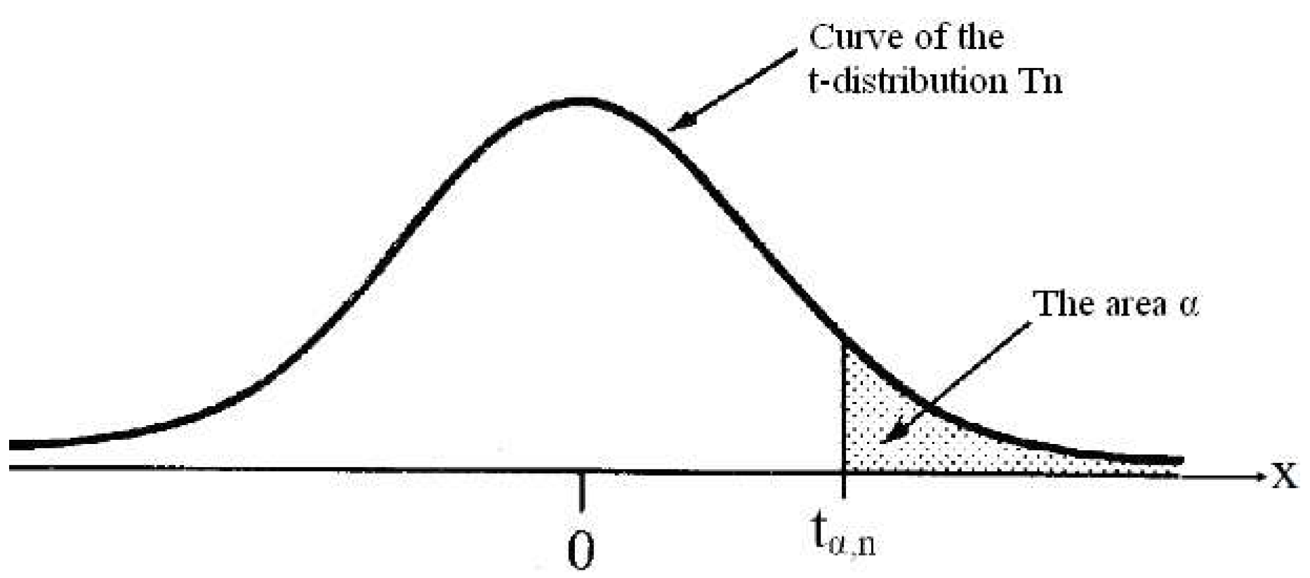
To evaluate the $100(1-\alpha )$ percentile in Figure 1, $t_{\alpha ,n}$ must be evaluated. The probability $P(T_n>t_{\alpha ,n})$ of the random variable $T_n$ with a t-distribution greater than $t_{\alpha ,n}$ is $\alpha$. To find $t_{\alpha ,n}$, (21) is used.

$$P(T_n>t_{\alpha ,n})=\alpha$$

(21)

or

$${\int }_{-\infty }^{t_{\alpha ,n}}{\displaystyle \frac{\Gamma \left(\right(n+1)/2)}{\sqrt{n\pi }\times \Gamma (n/2)\times (1+(x^2/n){)}^{(n+1)/2}}}dx=\alpha$$

(22)

where $\alpha$ is the function of $t_{\alpha ,n}$ in (22). The inverse function does not exist. That is found in Newton’s iteration method. Equation (22) is rewritten as

$$g(t_{\alpha ,n})={\int }_{-\infty }^{t_{\alpha ,n}}{\displaystyle \frac{\Gamma \left(\right(n+1)/2)}{\sqrt{n\pi }\times \Gamma (n/2)\times (1+(x^2/n){)}^{(n+1)/2}}}dx-\alpha$$

(23)

Then, to find $t_{\alpha ,n}$,

$$g\left(t_{\alpha ,n}\right)=0$$

(24)

To give a guess value $t_{\alpha ,n,0}$,

$$t_{\alpha ,n,new}=t_{\alpha ,n,old}-g\left(t_{\alpha ,n,old}\right)/g^{\prime }\left(t_{\alpha ,n,old}\right)$$

(25)

and the iteration is conducted. $g^{\prime }\left(t_{\alpha ,n,old}\right)$ in (26) is obtained by the following numerical differentiation.

$$g^{\prime }(t_{\alpha ,n,old})=\underset{\Delta t_{\alpha ,n}\to 0}{Lim}{\displaystyle \frac{g(t_{\alpha ,n,old}+\Delta t_{\alpha ,n})-g\left(t_{\alpha ,n,old}\right)}{\Delta t_{\alpha ,n}}}$$

(26)

Because the probability density function of the t-distribution is symmetric to x = 0, the five-point Gaussian integration method is adopted, and the interval (0,$t_{\alpha ,n}$) is divided into $10^6$ equally spaced subintervals. With a guess value of 1.0, $\Delta t_{\alpha ,n}$ in (27) is set to $0^{-5}$, and the iteration is stopped when the magnitude of $g(t_{\alpha ,n,old})/g^{\prime }(t_{\alpha ,n,old})$ becomes smaller than $10^{-5}$. The 100(1 − $\alpha$) percentile $t_{\alpha ,n}$ corresponds to the degrees of freedom n of 1 through 120, respectively, and $\alpha$ equal to 0.200, 0.100, 0.050, 0.025, 0.010, 0.005, 0.001, and 0.0005, respectively (

Table 2. The 100(1 − $\alpha$ ) percentile $t_{\alpha ,n}$ corresponding to the degrees of freedom n equal to 1 through 120, respectively, and $\alpha$ equal to 0.200, 0.100, 0.050, 0.025, 0.010, 0.005, 0.001, and 0.0005, respectively.

Degrees of Freedom n	$\mathit{\alpha }$
	0.200	0.100	0.050	0.025
1	1.3764	3.0777	6.3138	12.7062
2	1.0607	1.8856	2.9200	4.3027
3	0.9785	1.6377	2.3534	3.1824
4	0.9410	1.5332	2.1318	2.7764
5	0.9195	1.4759	2.0150	2.5706
6	0.9057	1.4398	1.9432	2.4469
7	0.8960	1.4149	1.8941	2.3646
8	0.8889	1.3968	1.8595	2.3060
9	0.8834	1.3830	1.8331	2.2622
10	0.8791	1.3722	1.8125	2.2281
15	0.8662	1.3406	1.7531	2.1315
20	0.8600	1.3253	1.7247	2.0860
30	0.8538	1.3104	1.6973	2.0423
40	0.8507	1.3031	1.6839	2.0211
60	0.8477	1.2958	1.6706	2.0003
80	0.8461	1.2922	1.6641	1.9901
100	0.8452	1.2901	1.6602	1.9840
120	0.8446	1.2886	1.6577	1.9799
Degrees of Freedom n	$\mathit{\alpha }$
	0.010	0.005	0.001	0.0005
1	31.8205	63.6567	318.3088	636.6192
2	6.9646	9.9248	22.3271	31.5991
3	4.5407	5.8409	10.2145	12.9240
4	3.7469	4.6041	7.1732	8.6103
5	3.3649	4.0321	5.8934	6.8688
6	3.1427	3.7074	5.2076	5.9588
7	2.9980	3.4995	4.7853	5.4079
8	2.8965	3.3554	4.5008	5.0413
9	2.8214	3.2498	4.2968	4.7809
10	2.7638	3.1693	4.1437	4.5869
15	2.6025	2.9467	3.7328	4.0728
20	2.5280	2.8453	3.5518	3.8495
30	2.4573	2.7500	3.3852	3.6460
40	2.4233	2.7045	3.3069	3.5510
60	2.3901	2.6603	3.2317	3.4602
80	2.3739	2.6387	3.1953	3.4163
100	2.3642	2.6259	3.1737	3.3905
120	2.3578	2.6174	3.1595	3.3735

).

4. Conclusions

The derivation process of the Gaussian numerical integration using (1)–(17) shows that when m = 2, two weight coefficients, w₁ and w₂, need to be determined at two sampling points, λ₁ and λ₂, resulting in four unknowns. The integrand is fitted as a cubic polynomial. Therefore, the form of the integrand in (1) is

$$f(\lambda )=\sum _{i=0}^{2m-1}{a}_i{\lambda }^i$$

(27)

where m is the number of sampling points in the Gaussian integral. Using (1) for integration, the theoretical error approaches zero even if the integration interval is not subdivided. However, since the probability density function of the t-distribution in (19) does not have the finite polynomial form as in (28), it is necessary to appropriately partition the integration interval before applying Gaussian integration with m sampling points and summing the results.

The probability density function $T_n\left(x\right)$ of the t-distribution with degrees of freedom n (19) indicates that the percentile $100(1-\alpha )$ $t_{\alpha ,n}$ for n = 1 is particularly difficult to calculate accurately, especially the $100(1-0.0005)$ percentile $t_{0.0005,1}=636.619$

The value is calculated to verify the correctness of the 100(1 − α) percentiles $t_{\alpha ,n}$ of the t-distribution listed in Table 2. The Newton–Raphson method is used to calculate the percentiles of the t-distribution (26) and (27), with an initial guess of 1.0 and an increment $\Delta t_{\alpha ,n}$ equal to $10^{-5}$ in (27). Iteration stops when the adjustment $g(t_{\alpha ,n,old})/g^{\prime }(t_{\alpha ,n,old})$ in (26) is smaller than a specified threshold $10^{-5}$.

For n = 1, $P(T_1>t_{0.0005,1})=\alpha =0.0005$. The Gaussian integration method is used with m = 5 sampling points, dividing the interval from 0 to the specified limit $t_{0.0005,1}$ into $10^6$ equal subintervals, and the result is $t_{0.0005,1}=636.619249$ after 15 iterations. The interval is partitioned from 0 to $t_{0.0005,1}$ into varying numbers of equal subintervals for NSECT = 100, 175, 250, 500, 750, 1000, 2500, 5000, $10^4$, $10^5$, $10^6$, and $10^7$, and the results are listed in

Table 3. The 100(1 – 0.0005) percentiles $t_{0.0005,1}$ by partitioning the interval from 0 to $t_{0.0005,1}$ into varying numbers of equal subintervals for NSECT = 100, 175, 250, 500, 750, 1000, 2500, 5000, $10^4$, $10^5$, $10^6$ and $10^7$.

NSECT	${\mathit{t}}_{0.0005,1}$	NSECT	${\mathit{t}}_{0.0005,1}$
100	574.327106	2500	636.619249
175	489.829447	5000	636.619249
250	599.936222	${10}^4$	636.619249
500	635.953237	${10}^5$	636.619249
750	636.635366	${10}^6$	636.619249
1000	636.621221	${10}^7$	636.619249

. Partitioning the interval into 1000 to 2500 subintervals yields the t-distribution’s 100(1 – 0.0005) percentile approaching 636.619249. Moreover, as the value of NSECT increases, the calculated result remains 636.619249, indicating that there is no issue with rounding errors in the computation process.

To verify the accuracy of $t_{0.0005,1}$ = 636.619249, $t_{0.0005,1}$ = 636.619249 in (23) for validation. The interval is partitioned from 0 to 636.619249 into various numbers of equal subintervals. NSECT = 100, 175, 250, 500, 750, 1000, 2500, 5000, $10^4$, $10^5$, $10^6$ and $10^7$, and the probability is $P(T_1>636.619249)$ that the random variable of the t-distribution exceeds 636.619249 (

Table 4. The probability $P(T_1>636.619249)$ that a random variable of the t-distribution exceeds the value 636.619249 by partitioning the interval from 0 to 636.619249 into various numbers of equal subintervals, NSECT = 100, 175, 250, 500, 750, 1000, 2500, 5000, ${10}^4$, $10^5$, $10^6$, and $10^7$.

NSECT	$\mathit{P}({\mathit{T}}_1>636.619249)$	NSECT	$\mathit{P}({\mathit{T}}_1>636.619249)$
100	−0.000585	2500	0.000500
175	0.000895	5000	0.000500
250	0.000527	${10}^4$	0.000500
500	0.000499	${10}^5$	0.000500
750	0.000500	${10}^6$	0.000500
1000	0.000500	${10}^7$	0.000500

). If the number of subintervals NSECT exceeds 750, the probability $P(T_1>636.619249)$ is accurately calculated as 0.000500.

The negative result for NSECT = 100 arises because 100 is too small, increasing error and yielding a probability $P(636.619249>T_1>0)$ greater than 0.5. Thus, it is reasonable to conclude that using increments $\Delta t_{\alpha ,n}$ as $10^{-5}$ in (27), stopping iteration when the adjustment $g(t_{\alpha ,n,old})/g^{\prime }(t_{\alpha ,n,old})$ in (26) is less than a specified threshold $10^{-5}$, and selecting an appropriate number ${10}^6$ of subintervals is valid. Each of the 100(1 − α) percentiles of the t-distribution in Table 2 is calculated in five seconds. Furthermore, rounding the values in Table 2 to three decimal places yields results that match exactly with those from highly authoritative publications [6].

References

- Montgomery, D.C. Design and Analysis of Experiments; John Wiley & Sons: New York, NY, USA, 2001. [Google Scholar]
- Lee, J.B.; Max, E. Introduction to Probability and Mathematical Statistics; Duxbury Press: Belmont, CA, USA, 1992. [Google Scholar]
- Jay, L.D. Probability and Statistics for Engineering and the Sciences; Brooks/Cole: Pacific Grove, CA, USA, 2012. [Google Scholar]
- Zienkiewicz, O.C. The Finite Element Method; McGraw-Hill Book Co.: Maidenhead, UK, 1977. [Google Scholar]
- Bathe, K.J. Finite Element Procedures in Engineering Analysis; Prentice-Hall: Upper Saddle River, NJ, USA, 1982. [Google Scholar]
- Pearson, E.S.; Hartley, H.O. Biometrika Tables for Statisticians; Cambridge University Press: Cambridge, UK, 1966. [Google Scholar]
Disclaimer/Publisher’s Note: The statements, opinions and data contained in all publications are solely those of the individual author(s) and contributor(s) and not of MDPI and/or the editor(s). MDPI and/or the editor(s) disclaim responsibility for any injury to people or property resulting from any ideas, methods, instructions or products referred to in the content. |
© 2025 by the author. Licensee MDPI, Basel, Switzerland. This article is an open access article distributed under the terms and conditions of the Creative Commons Attribution (CC BY) license (https://creativecommons.org/licenses/by/4.0/).