

Experimental and Modeled Assessment of Interventions to Reduce PM2.5 in a Residence during a Wildfire Event

Abstract
1. Introduction
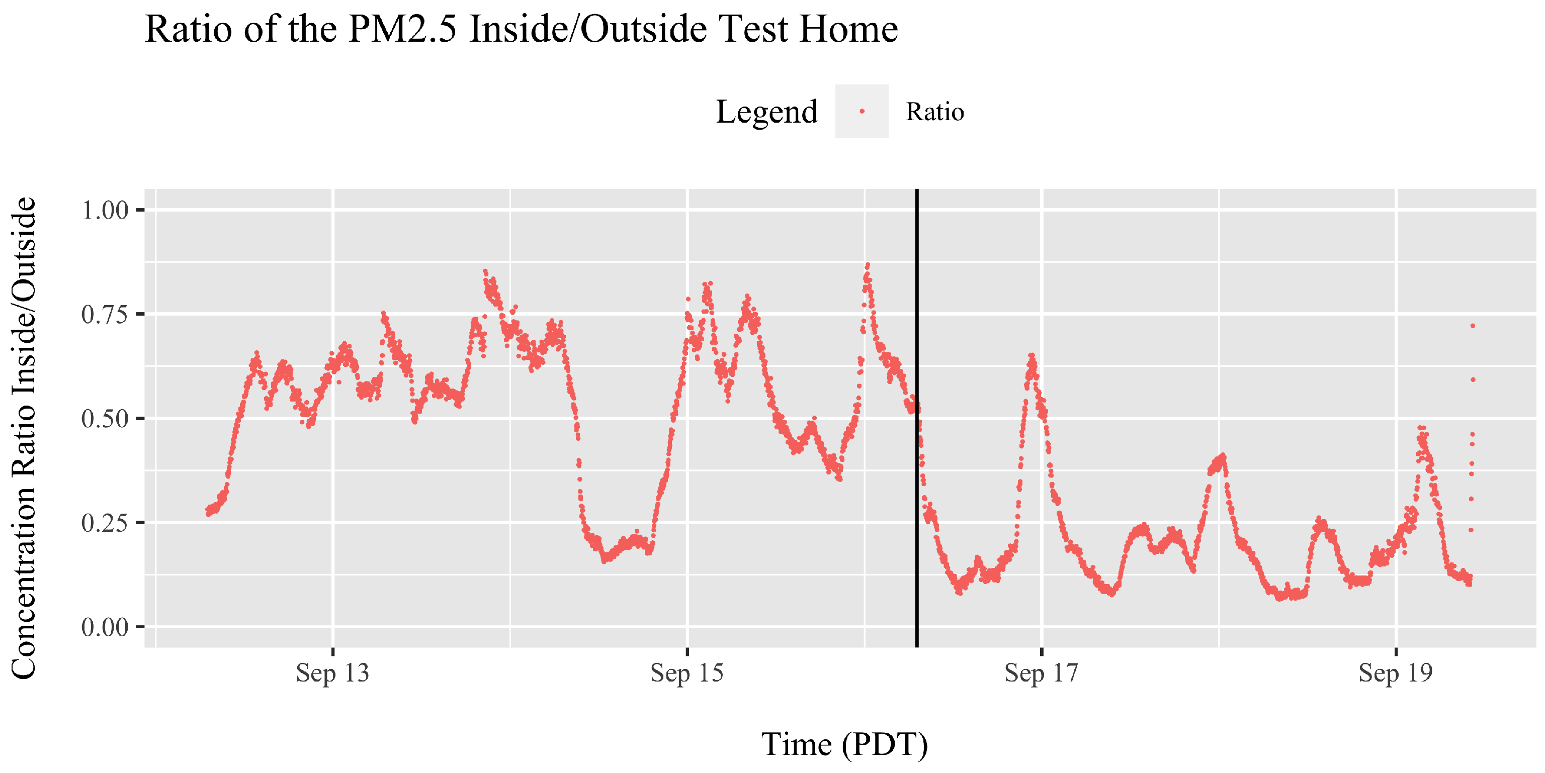
- What are the measured concentrations inside a home during a large fire event, and what is the ratio of indoor/outdoor (I/O) levels?
- How do interventions such as high-efficiency filtration and portable air cleaners impact indoor concentrations?
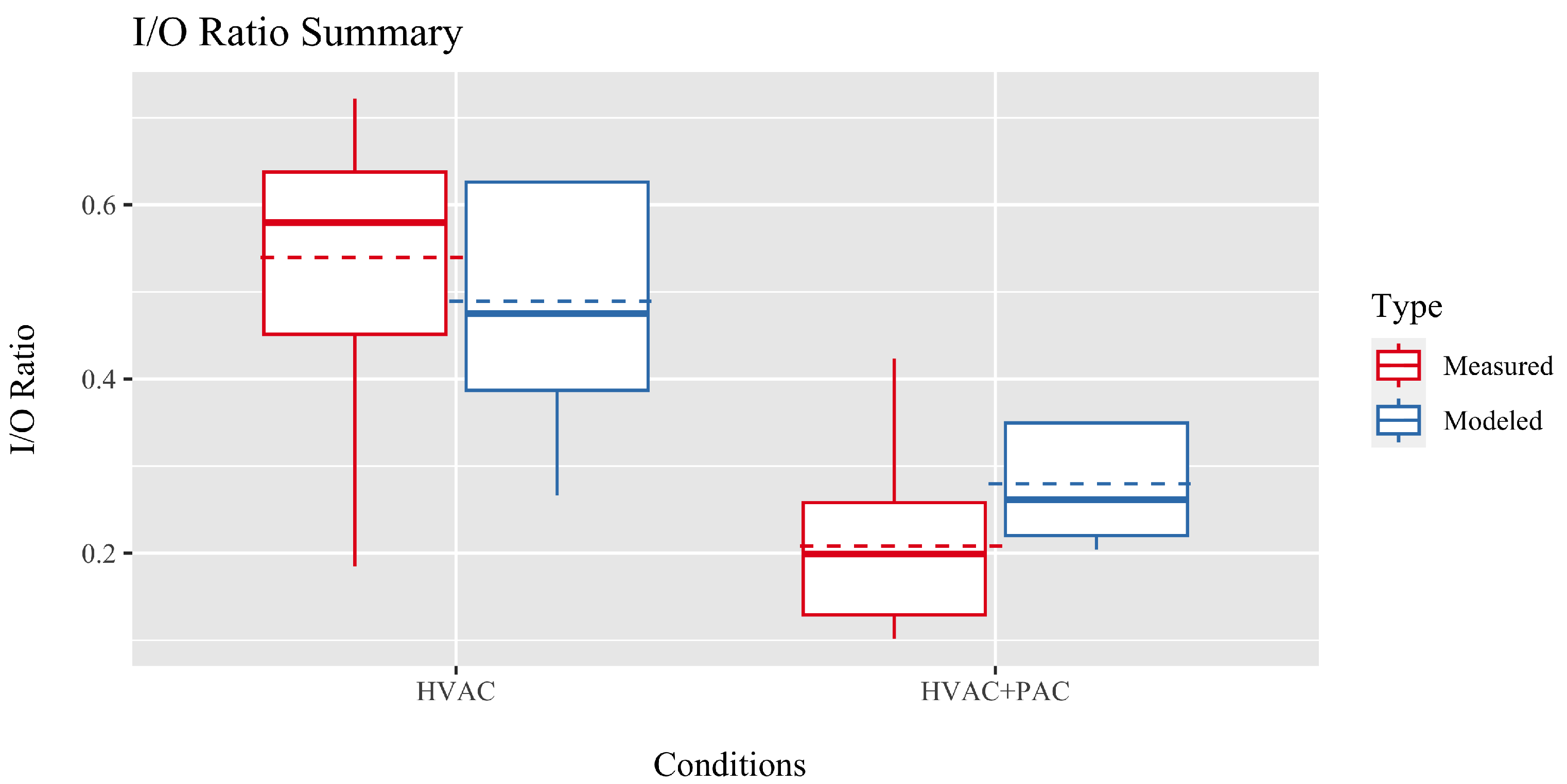
- How do empirical measurements of I/O ratios with indoor particle removal interventions compare to those predicted by mass balance modeling?
2. Background
3. Methods
3.1. Building Instrumentation and Pollutant Data Collection
3.1.1. Building Characteristics
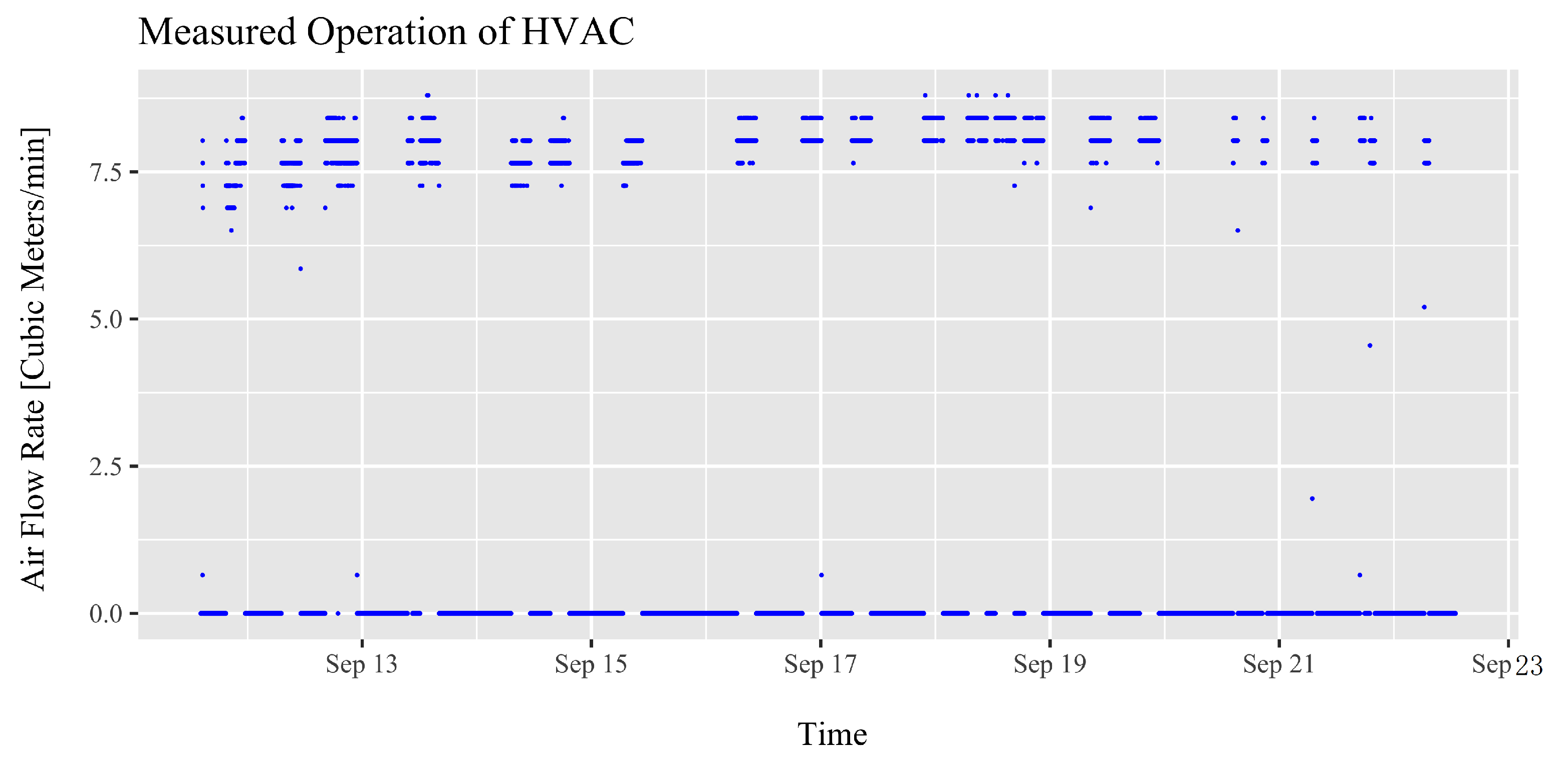
3.1.2. Air Leakage, Envelope Infiltration, HVAC Operation, and Portable Air Cleaner
3.1.3. Air Quality Measurements
3.2. Mass Balance Modeling
3.3. Sensitivity and Error
4. Results
4.1. Experimental Results
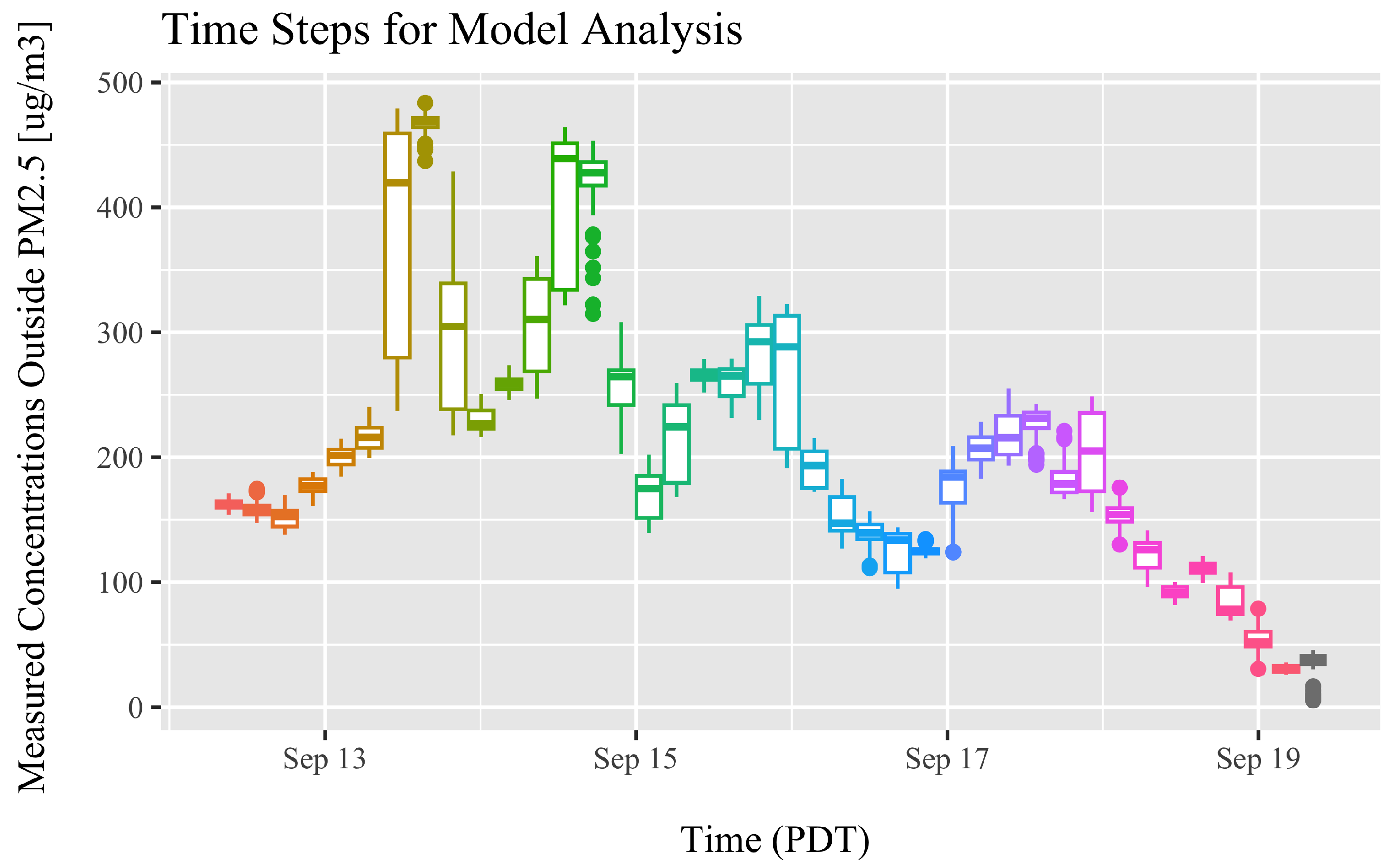
4.2. Quasi-Steady-State Time Increments
4.3. Modeling Results
4.4. Model Performance
5. Discussion
6. Conclusions
Author Contributions
Funding
Data Availability Statement
Acknowledgments
Conflicts of Interest
Abbreviations
| air changes per hour at 50 pascals | |
| AQI | air quality index |
| AFUE | annual fuel utilization efficiency |
| CADR | clean air delivery rate |
| CFA | central forced air |
| cubic feet per minute at 50 pascals | |
| DEQ | department of environmental quality |
| EPA | environmental protection agency |
| HVAC | heating, ventilation, and air conditioning |
| I/O | indoor/outdoor ratio |
| MAE | mean absolute error |
| MERV | minimum efficiency reporting value |
| PAC | portable air cleaner |
| RMSE | root mean square error |
| SD | standard deviation |
| SEER | seasonal energy efficiency ratio |
| VOCs | volatile organic compounds |
References
- Barbero, R.; Abatzoglou, J.T.; Larkin, N.K.; Kolden, C.A.; Stocks, B. Climate change presents increased potential for very large fires in the contiguous United States. Int. J. Wildland Fire 2015, 24, 892–899. [Google Scholar] [CrossRef]
- Liu, Y.; Stanturf, J.; Goodrick, S. Trends in global wildfire potential in a changing climate. For. Ecol. Manag. 2010, 259, 685–697. [Google Scholar] [CrossRef]
- Jaffe, D.A.; O’Neill, S.M.; Larkin, N.K.; Holder, A.L.; Peterson, D.L.; Halofsky, J.E.; Rappold, A.G. Wildfire and prescribed burning impacts on air quality in the United States. J. Air Waste Manag. Assoc. 2020, 70, 583–615. [Google Scholar] [CrossRef] [PubMed]
- Sidhu, K.S.; Hesse, J.L.; Bloomer, A.W. Indoor Air: Potential Health Risks Related to Residential Wood Smoke, as Determined under the Assumptions of the US EPA Risk Assessment Model. Indoor Environ. 1993, 2, 92–97. [Google Scholar] [CrossRef]
- Aguilera, R.; Corringham, T.; Gershunov, A.; Benmarhnia, T. Wildfire smoke impacts respiratory health more than fine particles from other sources: Observational evidence from Southern California. Nat. Commun. 2021, 12, 1493. [Google Scholar] [CrossRef] [PubMed]
- Anjali, H.; Muhammad, A.; Anthony, D.M.; Karen, S.; Sim, R.; Mick, M.; Tonkin, A.M.; Abramson, M.J.; Martine, D. Impact of Fine Particulate Matter (PM2.5) Exposure During Wildfires on Cardiovascular Health Outcomes. J. Am. Heart Assoc. 2019, 4, e001653. [Google Scholar] [CrossRef]
- Johnston, F.; Hanigan, I.; Henderson, S.; Morgan, G.; Bowman, D. Extreme air pollution events from bushfires and dust storms and their association with mortality in Sydney, Australia 1994–2007. Environ. Res. 2011, 111, 811–816. [Google Scholar] [CrossRef]
- Richardson, L.A.; Champ, P.A.; Loomis, J.B. The hidden cost of wildfires: Economic valuation of health effects of wildfire smoke exposure in southern California. J. For. Econ. 2012, 18, 14–35. [Google Scholar] [CrossRef]
- Fann, N.; Alman, B.; Broome, R.A.; Morgan, G.G.; Johnston, F.H.; Pouliot, G.; Rappold, A.G. The health impacts and economic value of wildland fire episodes in the U.S.: 2008–2012. Sci. Total. Environ. 2018, 610–611, 802–809. [Google Scholar] [CrossRef]
- Tsoulou, I.; He, R.; Senick, J.; Mainelis, G.; Andrews, C.J. Monitoring summertime indoor overheating and pollutant risks and natural ventilation patterns of seniors in public housing. Indoor Built Environ. 2023, 32, 992–1019. [Google Scholar] [CrossRef]
- Holm, S.M.; Miller, M.D.; Balmes, J.R. Health effects of wildfire smoke in children and public health tools: A narrative review. J. Expo. Sci. Environ. Epidemiol. 2021, 31, 1–20. [Google Scholar] [CrossRef] [PubMed]
- Holstius, D.M.; Reid, C.E.; Jesdale, B.M.; Morello, F.R. Birth Weight following Pregnancy during the 2003 Southern California Wildfires. Environ. Health Perspect. 2012, 120, 1340–1345. [Google Scholar] [CrossRef] [PubMed]
- Hanigan, I.C.; Johnston, F.H.; Morgan, G.G. Vegetation fire smoke, indigenous status and cardio-respiratory hospital admissions in Darwin, Australia, 1996–2005: A time-series study. Environ. Health 2008, 7, 42. [Google Scholar] [CrossRef] [PubMed]
- Rappold, A.G.; Cascio, W.E.; Kilaru, V.J.; Stone, S.L.; Neas, L.M.; Devlin, R.B.; Diaz-Sanchez, D. Cardio-respiratory outcomes associated with exposure to wildfire smoke are modified by measures of community health. Environ. Health 2012, 11, 71. [Google Scholar] [CrossRef] [PubMed]
- Shrestha, P.M.; Humphrey, J.L.; Carlton, E.J.; Adgate, J.L.; Barton, K.E.; Root, E.D.; Miller, S.L. Impact of Outdoor Air Pollution on Indoor Air Quality in Low-Income Homes during Wildfire Seasons. Int. J. Environ. Res. Public Health 2019, 16, 3535. [Google Scholar] [CrossRef] [PubMed]
- Burke, M.; Heft-Neal, S.; Li, J.; Driscoll, A.; Baylis, P.; Stigler, M.; Weill, J.A.; Burney, J.A.; Wen, J.; Childs, M.L.; et al. Exposures and behavioural responses to wildfire smoke. Nat. Hum. Behav. 2022, 6, 1351–1361. [Google Scholar] [CrossRef]
- Antonopoulos, C.A.; Dillon, H.E.; Dzombak, R.; Heslam, D.; Salzman, M.; Kappaz, P.; Rosenberg, S.I. Pushing Green: Leveraging Home Energy Score to Promote Deep-Energy Retrofits in Portland, Oregon; Technical Report PNNL-SA-152375; Pacific Northwest National Lab. (PNNL): Richland, WA, USA, 2020. [Google Scholar]
- Fisk, W.J.; Chan, W.R. Health benefits and costs of filtration interventions that reduce indoor exposure to PM2.5 during wildfires. Indoor Air 2017, 27, 191–204. [Google Scholar] [CrossRef]
- Nazarenko, Y.; Pal, D.; Ariya, P.A. Air quality standards for the concentration of particulate matter 2.5, global descriptive analysis. Bull. World Health Organ. 2021, 99, 125–137D. [Google Scholar] [CrossRef]
- Ryan, R.G.; Silver, J.D.; Schofield, R. Air quality and health impact of 2019–20 Black Summer megafires and COVID-19 lockdown in Melbourne and Sydney, Australia. Environ. Pollut. 2021, 274, 116498. [Google Scholar] [CrossRef]
- Barn, P.K.; Elliott, C.T.; Allen, R.W.; Kosatsky, T.; Rideout, K.; Henderson, S.B. Portable air cleaners should be at the forefront of the public health response to landscape fire smoke. Environ. Health 2016, 15, 116. [Google Scholar] [CrossRef]
- Henderson, D.E.; Milford, J.B.; Miller, S.L. Prescribed Burns and Wildfires in Colorado: Impacts of Mitigation Measures on Indoor Air Particulate Matter. J. Air Waste Manag. Assoc. 2005, 55, 1516–1526. [Google Scholar] [CrossRef] [PubMed]
- Bai, L.; Yu, C.W. Towards the future prospect of control technology for alleviating indoor air pollution. Indoor Built Environ. 2021, 30, 871–874. [Google Scholar] [CrossRef]
- O’Dell, K.; Ford, B.; Burkhardt, J.; Magzamen, S.; Anenberg, S.C.; Bayham, J.; Fischer, E.V.; Pierce, J.R. Outside in: The relationship between indoor and outdoor particulate air quality during wildfire smoke events in western US cities. Environ. Res. Health 2022, 1, 015003. [Google Scholar] [CrossRef]
- Kirk, W.M.; Fuchs, M.; Huangfu, Y.; Lima, N.; O’Keeffe, P.; Lin, B.; Jobson, T.; Pressley, S.; Walden, V.; Cook, D.; et al. Indoor air quality and wildfire smoke impacts in the Pacific Northwest. Sci. Technol. Built Environ. 2018, 24, 149–159. [Google Scholar] [CrossRef]
- Liang, Y.; Sengupta, D.; Campmier, M.J.; Lunderberg, D.M.; Apte, J.S.; Goldstein, A.H. Wildfire smoke impacts on indoor air quality assessed using crowdsourced data in California. Proc. Natl. Acad. Sci. USA 2021, 118, e2106478118. [Google Scholar] [CrossRef] [PubMed]
- Xiang, J.; Huang, C.H.; Shirai, J.; Liu, Y.; Carmona, N.; Zuidema, C.; Austin, E.; Gould, T.; Larson, T.; Seto, E. Field measurements of PM2.5 infiltration factor and portable air cleaner effectiveness during wildfire episodes in US residences. Sci. Total Environ. 2021, 773, 145642. [Google Scholar] [CrossRef]
- Reisen, F.; Powell, J.C.; Dennekamp, M.; Johnston, F.H.; Wheeler, A.J. Is remaining indoors an effective way of reducing exposure to fine particulate matter during biomass burning events? J. Air Waste Manag. Assoc. 2019, 69, 611–622. [Google Scholar] [CrossRef]
- US EPA. Wildfires and Indoor Air Quality (IAQ); US EPA: Washington, DC, USA, 2018.
- Jones, A.P. Indoor air quality and health. Atmos. Environ. 1999, 33, 4535–4564. [Google Scholar] [CrossRef]
- Nazaroff, W.W. Indoor particle dynamics. Indoor Air 2004, 14 (Suppl. 7), 175–183. [Google Scholar] [CrossRef]
- Laverge, J.; Van Den Bossche, N.; Heijmans, N.; Janssens, A. Energy saving potential and repercussions on indoor air quality of demand controlled residential ventilation strategies. Build. Environ. 2011, 46, 1497–1503. [Google Scholar] [CrossRef]
- Fisk, W.J.; Singer, B.C.; Chan, W.R. Association of residential energy efficiency retrofits with indoor environmental quality, comfort, and health: A review of empirical data. Build. Environ. 2020, 180, 107067. [Google Scholar] [CrossRef]
- Guyot, G.; Sherman, M.H.; Walker, I.S. Smart ventilation energy and indoor air quality performance in residential buildings: A review. Energy Build. 2018, 165, 416–430. [Google Scholar] [CrossRef]
- Singer, B.C.; Chan, W.R.; Kim, Y.S.; Offermann, F.J.; Walker, I.S. Indoor air quality in California homes with code-required mechanical ventilation. Indoor Air 2020, 30, 885–899. [Google Scholar] [CrossRef]
- Antonopoulos, C.A.; Rosenberg, S.I.; Zhao, H.; Walker, I.S.; Delp, W.W.; Chan, W.R.; Singer, B.C. Mechanical ventilation and indoor air quality in recently constructed U.S. homes in marine and cold-dry climates. Build. Environ. 2023, 245, 110480. [Google Scholar] [CrossRef]
- Wallner, P.; Munoz, U.; Tappler, P.; Wanka, A.; Kundi, M.; Shelton, J.F.; Hutter, H.P. Indoor Environmental Quality in Mechanically Ventilated, Energy-Efficient Buildings vs. Conventional Buildings. Int. J. Environ. Res. Public Health 2015, 12, 14132–14147. [Google Scholar] [CrossRef]
- US Department of Energy Prototype Building Models|Building Energy Codes Program. Available online: https://www.energycodes.gov/prototype-building-models (accessed on 29 October 2023).
- State of Oregon Department of Environmental Quality: Air Quality Monitoring and Facility Locations Map. Available online: https://www.oregon.gov/deq/aq/Pages/Air-Quality-Map.aspx (accessed on 3 November 2023).
- ASTM International. Standard Test Method for Determining Air Leakage Rate by Fan Pressurization. ASTM E779-10. Available online: https://www.astm.org/e0779-10.html (accessed on 29 October 2023).
- Lai, Y.; Ridley, I.; Brimblecombe, P. Blower-door estimates of PM2.5 deposition rates and penetration factors in an idealized room. Indoor Built Environ. 2022, 31, 2064–2082. [Google Scholar] [CrossRef]
- Sherman, M.H. Estimation of infiltration from leakage and climate indicators. Energy Build. 1987, 10, 81–86. [Google Scholar] [CrossRef]
- AHAM. CADR Certified Air Cleaners. Available online: https://www.ahamdir.com/room-air-cleaners/ (accessed on 29 October 2023).
- Delp, W.W.; Singer, B.C. Wildfire Smoke Adjustment Factors for Low-Cost and Professional PM2.5 Monitors with Optical Sensors. Sensors 2020, 20, 3683. [Google Scholar] [CrossRef]
- Holder, A.L.; Mebust, A.K.; Maghran, L.A.; McGown, M.R.; Stewart, K.E.; Vallano, D.M.; Elleman, R.A.; Baker, K.R. Field Evaluation of Low-Cost Particulate Matter Sensors for Measuring Wildfire Smoke. Sensors 2020, 20, 4796. [Google Scholar] [CrossRef]
- 2021 Wildfire Calibrations|Clarity Movement Co. Available online: https://www.clarity.io/2021-wildfire-calibrations (accessed on 29 October 2023).
- Novoselac, A.; Siegel, J.A. Impact of placement of portable air cleaning devices in multizone residential environments. Build. Environ. 2009, 44, 2348–2356. [Google Scholar] [CrossRef]
- Vershaw, J.; Choinowski, D.; Siegel, J.; Nigro, P. Implications of Filter Bypass. ASHRAE Trans. 2009, 115, 191–198. [Google Scholar]
- Azimi, P.; Zhao, D.; Stephens, B. Estimates of HVAC filtration efficiency for fine and ultrafine particles of outdoor origin. Atmos. Environ. 2014, 98, 337–346. [Google Scholar] [CrossRef]
- Dillon, M.B.; Sextro, R.G.; Delp, W.W. Protecting building occupants against the inhalation of outdoor-origin aerosols. Atmos. Environ. 2022, 268, 118773. [Google Scholar] [CrossRef]
- Kutz, J.N. Data-Driven Modeling & Scientific Computation: Methods for Complex Systems & Big Data; Oxford University Press: Oxford, UK; New York, NY, USA, 2013. [Google Scholar]
- Zhao, H.; Stephens, B. Using portable particle sizing instrumentation to rapidly measure the penetration of fine and ultrafine particles in unoccupied residences. Indoor Air 2017, 27, 218–229. [Google Scholar] [CrossRef]
- Walker, I.; Sherman, M.; Joh, J.; Chan, W.R. Applying Large Datasets toDeveloping a Better Understanding of Air Leakage Measurement in Homes. Int. J. Vent. 2013, 11, 323–338. [Google Scholar] [CrossRef]
- ResStock Analysis Tool. Available online: https://www.nrel.gov/buildings/resstock.html (accessed on 29 October 2023).
- Azimi, P.; Zhao, D.; Stephens, B. Modeling the impact of residential HVAC filtration on indoor particles of outdoor origin (RP-1691). Sci. Technol. Built Environ. 2016, 22, 431–462. [Google Scholar] [CrossRef]
- Luo, N.; Weng, W.; Xu, X.; Hong, T.; Fu, M.; Sun, K. Assessment of occupant-behavior-based indoor air quality and its impacts on human exposure risk: A case study based on the wildfires in Northern California. Sci. Total Environ. 2019, 686, 1251–1261. [Google Scholar] [CrossRef]
- Farbotko, C.; Waitt, G. Residential air-conditioning and climate change: Voices of the vulnerable. Health Promot. J. Aust. 2011, 22, 13–15. [Google Scholar] [CrossRef]
- Goldsworthy, M.; Poruschi, L. Air-conditioning in low income households; a comparison of ownership, use, energy consumption and indoor comfort in Australia. Energy Build. 2019, 203, 109411. [Google Scholar] [CrossRef]


| Characteristic | Value |
|---|---|
| Year Built | 1928 |
| Home Size () | 243 |
| Volume () | 457 |
| Attached Garage | No |
| Stories | 2 |
| Number of Occupants: Pets | 3:2 |
| Blower Door Results (:) | 2355:9 |
| Measurement Device | Parameters | Accuracy | Resolution | Sampling Locations |
|---|---|---|---|---|
| Onset HOBO UX100-011 | T, RH | C from 0 to C | 1 min | Indoor: central |
| Onset HOBO U23 Pro v2 | % from 10% to 90%; | Outdoor | ||
| up to % at C including hysteresis | ||||
| Clarity Node | , , | 0–450 g/ for | 2 min | Indoor: central; |
| Outdoor: backyard | ||||
| Digi-Sense Vane Anemometer WD-20250 | HVAC airflows | Air velocity: ±(3% + 0.2 m/s); | Indoor: living and dining room registers |
| HVAC | HVAC+PAC | |
|---|---|---|
| Central forced air system operation | Intermittent | Intermittent |
| Efficiency of filter in central forced air system | Upgraded to High (MERV 13) | Upgraded to High (MERV 13) |
| Continuously operating portable air cleaner? | No | Yes |
| Experiment timeframe | 9/12–9/16 | 9/16–9/18 |
| Parameter | Units | Values | Description |
|---|---|---|---|
| 1/h | 0.71 * | Estimated annual infiltration rate. Calculated from blower door value | |
| 1/h | 0.39 [18] | Rate of particle removal by deposition on surfaces | |
| P | - | 0.82 [50] | Particle penetration factor |
| 1/h | 4.96 ** | Recirculation air flow rate of the HVAC normalized by volume | |
| D | - | 0.28 average * | Duty cycle. Experiment time series calculation discussed in Section 4.1 |
| - | 0.30 | HVAC filter efficiency for . Determined from MERV rating using published methods [48,49] | |
| 1/h | 0.87 ** | PAC filter efficiency for multiplied by the air flow rate of the portable air cleaner normalized by volume. Determined from manufacturer CADR specifications for portable air cleaner | |
| V | 456 * | Volume of the house | |
| g/ | Experiment time series measurement as shown in Section 4.1. | Outside particle concentration |
| Parameter | Units | Max Sensitivity [% I/O Ratio Variation] |
|---|---|---|
| 1/h | 6.75–7.17 | |
| 1/h | 1.65–1.70 | |
| P | - | 3.1–10 |
| 1/h | 2.9–3.1 | |
| D | - | 2.9–3.1 |
| - | 2.9–3.1 | |
| 1/h | 2.25–2.35 | |
| V | 5.04–5.54 |
| Parameter | Without Portable Air Cleaner (HVAC) [g/] | With Portable Air Cleaner (HVAC+PAC) [g/] |
|---|---|---|
| Outdoor Mean | 259.9 | 135.1 |
| Outdoor Median | 241.4 | 134.8 |
| Outdoor Range (min–max) | 138.0–483.7 | 5.4–254.9 |
| Indoor Mean | 134.4 | 30.2 |
| Indoor Median | 121.8 | 24.1 |
| Indoor Range (min–max) | 56.53–262.93 | 10.4–72.1 |
| Mean I/O Ratio | 0.55 | 0.21 |
| Median I/O Ratio | 0.58 | 0.18 |
| Intervention | Intermittent High-Capture Filter (MERV 13)
(HVAC) | Intermittent High-Capture Filter Plus PAC
(HVAC+PAC) |
|---|---|---|
| Mean measured indoor concentration (g/) | 134.9 (n = 2169) | 28.2 (n = 1706) |
| Mean measured indoor/outdoor ratio | 0.55 (n = 2169) | 0.22 (n = 1706) |
| Mean indoor/outdoor ratio: modeled and standard deviation | 0.48 SD 0.13 (n = 23) | 0.28 SD 0.06 (n = 16) |
| HVAC | HVAC + PAC | |
|---|---|---|
| RMSE [g/] | 50.24 | 17.43 |
| MAE [g/] | 38.89 | 13.03 |
Disclaimer/Publisher’s Note: The statements, opinions and data contained in all publications are solely those of the individual author(s) and contributor(s) and not of MDPI and/or the editor(s). MDPI and/or the editor(s) disclaim responsibility for any injury to people or property resulting from any ideas, methods, instructions or products referred to in the content. |
© 2024 by the authors. Licensee MDPI, Basel, Switzerland. This article is an open access article distributed under the terms and conditions of the Creative Commons Attribution (CC BY) license (https://creativecommons.org/licenses/by/4.0/).
Share and Cite
Antonopoulos, C.; Dillon, H.E.; Gall, E. Experimental and Modeled Assessment of Interventions to Reduce PM2.5 in a Residence during a Wildfire Event. Pollutants 2024, 4, 26-41. https://doi.org/10.3390/pollutants4010003
Antonopoulos C, Dillon HE, Gall E. Experimental and Modeled Assessment of Interventions to Reduce PM2.5 in a Residence during a Wildfire Event. Pollutants. 2024; 4(1):26-41. https://doi.org/10.3390/pollutants4010003
Chicago/Turabian StyleAntonopoulos, Chrissi, H. E. Dillon, and Elliott Gall. 2024. "Experimental and Modeled Assessment of Interventions to Reduce PM2.5 in a Residence during a Wildfire Event" Pollutants 4, no. 1: 26-41. https://doi.org/10.3390/pollutants4010003
APA StyleAntonopoulos, C., Dillon, H. E., & Gall, E. (2024). Experimental and Modeled Assessment of Interventions to Reduce PM2.5 in a Residence during a Wildfire Event. Pollutants, 4(1), 26-41. https://doi.org/10.3390/pollutants4010003