Abstract
The response of aquifers with contrasting climate and geology to climate and land cover change perturbations through natural groundwater recharge remains inadequately understood. In Tanzania and elsewhere in the world, studies have been conducted to assess the impact of climate change and variability, and land use/cover changes on stream flow using different models, but similar studies on groundwater dynamics are inadequate. This study, therefore, examined the influence of land use/cover and climate dynamics on natural groundwater recharge in basins with contrasting climate and geology in Tanzania, applying the modified soil moisture balance method, coupled with the curve number (CN). The method hinges on the balance between the incoming water from precipitation and the outflow of water by evapotranspiration. The different parameters in the soil moisture balance method were computed using the Thornthwaite Water Balance software. The potential evapotranspiration (PET) was calculated using the daily maximum and minimum temperatures, utilizing two-temperature-based PET methods, Penman–Monteith (PM) and Hargreaves–Samani (HS). The rainfall data were obtained from the gauging stations under the Tanzania Meteorological Agency and some additional data were acquired from climate observatories management by water basins. The results show that there has been a quasi-stable CN in the Singida semi-arid, fractured crystalline basement aquifer (74.2 in 1997, 73.64 in 2005, and 73.87 in 2018). In the Kimbiji, humid, Neogene sedimentary aquifer, the CN has been steadily increasing (66.69 in 1997, 69.08 in 2008, and 71.42 in 2016), indicating the rapid land cover changes in the Kimbiji aquifer as compared to the Singida aquifer. For the Kimbiji humid aquifer, the PET calculated using the Penman–Monteith (PM) method for the 1996/1997, 2007/2008, and 2015/2016 hydrological years were 1156.5, 1079.5, and 1143.9 mm/year, respectively, while for the Hargreaves–Samani (HS) method, the PET was found to be 1046.1, 1138.3, and 1204.4 mm/year for the 1996/1997, 2007/2008, and 2015/2016 hydrological years, respectively. For the Singida semi-arid aquifer, the PM PET method resulted in 2083.3, 2053.6, and 1875.4 mm/year for the 1996/1997, 2004/2005, and 2017/2018 hydrological years, respectively. The HS method produced relatively lower PET values for the semi-arid area (1839.4, 1814.7, and 1710.2 mm/year) for the 1996/1997, 2004/2005, and 2017/2018 hydrological years, respectively. It was equally revealed that the recharge and aridity indices correspond with the PET calculated using two temperature-dependent methods. The decline of certain land covers (forests) and increase in others (built-up areas) have contributed to the increase in surface runoff in each study area, possibly resulting in the decreasing trend of groundwater recharge. An overestimation of the PET using the HS method in the Kimbiji humid aquifer was observed, which was relatively smaller than the overestimation of the PET using the PM method in the Singida semi-arid aquifer. Despite the difference in climate and geology, the response of the two aquifers to rainfall is similar. The combined influence of climate and land cover changes on natural groundwater recharge was observed to be prominent in the Kimbiji aquifer, while only climate variability appreciably influences natural groundwater recharge in the Singida semi-arid aquifer. El Nino and the Southern Oscillation as part of the climate variability phenomenon dwarfed the time lags between rainfall and recharge in the two basins, regardless of their difference in climate and geology.
1. Background Information
There are considerable stresses on the groundwater systems, both natural (e.g., climate variability and change) and human-induced (land use/cover changes, population increase). Those stresses have raised concerns about the long-term sustainability of groundwater resources for various uses all over the world. Reportedly, land use/cover change and climate variability perturbations have knock-on effects on natural groundwater recharge [1], but the spatial and temporal extents of such effects in basins with contrasting climate and geology are poorly understood and documented [2,3]. This makes it hard to design succinct groundwater management plans that accommodate the difference in climate and geology. Arguably, the management of groundwater is often carried out with inadequate knowledge of the relationship between groundwater recharge and other climatic and non-climatic factors, resulting in overexploitation, double accounting and an unsatisfactory estimation of natural groundwater recharge in most basins, as had previously been pointed out [4]. The impacts of land use/cover changes and climate variability and change on surface water are receiving appreciable scientific attention as argued recently [5], but the attention on groundwater is relatively insufficient. This contention was supported previously by other researchers [6,7], and recently by Sterling et al. [8], who pointed out that globally, the impacts of land use/land cover changes on the atmospheric components of the hydrologic cycle are increasingly recognized. It was hinted further that most hydrologic models mainly focus on river flows and discharge and not on changes in groundwater recharge and storages [9].
In Tanzania, several studies have been conducted to assess the impact of climate change and variability, and land use/cover changes on stream flow using different models. Such studies were conducted in the Ngerengere sub-basin [5], in the Wami River sub-basin [10], in the Pangani basin [11], and in the Wami river sub-basin [12]. Moreover, Mbungu and Kashaigili [13] carried out hydrological modeling in the Little Ruaha River watershed, assessing the impact of climate and land cover changes on stream flow. Other researchers [14,15] carried out hydrological studies in the Mbarali River and Wami river subbasins, respectively, highlighting the impacts of climate change and landcover dynamics on river flows. The consequences of land cover dynamics on catchment hydrology have equally been conducted in the Little Ruaha River catchment [16]. Some studies, albeit scanty, that aimed at assessing the impact of land cover changes on groundwater recharge in Tanzania have been carried out in the northern part of Tanzania recently [17,18]. Nonetheless, the paucity of studies on the implication of climate variability/change and land use/cover changes on natural groundwater recharge, considering the difference in geology and climate in responding to such perturbations, remains ostensibly clear.
Debatably, groundwater recharge is positively related to rainfall as decreasing precipitation is said to contribute more to decreasing groundwater table levels [9,19]. Nevertheless, this may not be scientifically true altogether as other factors come into play and the relation between rainfall and natural groundwater recharge may not be linear. This information underscores the fact that the relationship between rainfall and groundwater recharge is becoming more complex as opined by other studies [20]. The difference in climate and geology adds up to that complexity. The literature, therefore, divulges inadequate scientific works regarding the impact of spatiotemporal climate and land use/cover changes on natural groundwater recharge and groundwater resources in general, despite some patches of works.
The observed paucities and gaps, therefore, call for a combination of empirical and conceptual approaches to establish a more robust, scientifically plausible trend and status, which take into account more factors other than rainfall alone. This study thus attempted to quantitatively evaluate the spatial and temporal variations of groundwater recharge under different geological and climatic conditions. The influence of climate variability and land cover changes on groundwater recharge were independently assessed, utilizing the Singida semi-arid, fractured crystalline basement and the Kimbiji, humid, Neogene sedimentary coastal aquifers as test cases.
2. Description of the Study Areas
2.1. Climate
The Singida aquifer (Figure 1A), found in the Internal Drainage Basin (IDB), central Tanzania (See Figure 1C) receives an average rainfall of 500–800 mm annually, and it experiences a unimodal rainfall season, beginning in November and lasting until May. The annual evapotranspiration can be as high as 1800 mm per year. Although there are humid months, generally the area is typically semi-arid, with an average aridity index of 0.49. Due to a complete absence of rainfall in some months, there can be hyper-arid conditions in Singida. The area experiences very high evapotranspiration rates, usually above 100 mm/month throughout the year [21]. Day temperatures range between 25 and 30 °C, while night temperatures may drop down to 12 °C. The months of June, July, August, and September are the driest of all. Generally, the area falls within the driest zone of the Internal Drainage Basin (IDB), and hence the main source of water is groundwater (deep and shallow wells).
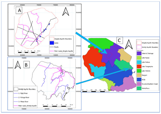
Figure 1.
Maps showing the position of the two study areas (A,B) in relation to the Wami-Ruvu basin and the Country (C).
With relatively higher long term mean annual evapotranspiration (approximately 1400 mm/year) than mean annual rainfall (1100 mm/year), the Kimbiji aquifer (Figure 1B), located in the eastern part of Tanzania towards the Indian Ocean (Figure 1C), is characterized by a humid climate. Contrary to the Singida semi-arid aquifer, where there can be hyper aridity conditions from June to September, the Kimbiji aquifer can only experience slight semi-arid conditions from June to October, and then around January. The air temperatures, both maximum and minimum, indicate that the area is generally warm. The mean monthly maximum temperature can be as high as 32 °C, while the lowest mean monthly minimum temperature can be 19 °C, compared to 12 °C, which is the lowest mean monthly minimum temperature in the Singida aquifer. This aquifer really occurs in a warm and humid climate as reported recently [21].
2.2. Geology
Geologically, the Singida aquifer is found within six main geological units, which include some small lakes denoted as Lk (Figure 2). The main geological units are plutonic rocks consisting of granite and granodiorite, foliated, gneissose, or migmatitic, and some massive porphiyroblastic, including intimately related regional migmatite. Lithologically, these are of two types, (i) those with a topographic rough texture (gs) and (ii) strongly weathered granite with a smooth topographic texture (gs-b). There is a Nyanzan system (Z) that occupies the central part of the study area, and extends east–west, and north–east, which is made up of banded ironstone, metavolcanics, chlorite schist, and pseudo-porphyry (Figure 2). Patches of Cenozoic sediments classified into (N), which are mostly alkaline volcanics in the north, north-eastern, central, and western parts of the study area, characterized by olivine basalt, alkali basalt, phonolite, trachyte, nephelinenite and pyroclastics, and (NI), made up of lacustrine, sand, silt, limestone, and tuff, which can be observed in the southern, western, and north-western parts of the study area. There are also lineaments extending north–south, north-east, south-west with some branching to the south-east and north-west.
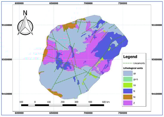
Figure 2.
The geology of the Singida aquifer and the lineament system distribution.
The Kimbiji coastal Neogene aquifer (Figure 3) is made up of Beach sand dune (b) and fluvial deposits (r1). These are younger (Quaternary) than any other geological units in the Kimbiji aquifer. This study area is also made up of Terrace deposits (Nt) and Fluvial marine sand (Nf). These are of a tertiary time scale. Fringes of continental and marine sandstone (C) in the Cretaceous age are also found in the Kimbiji aquifer system. Generally, the geology of the Kimbiji, humid, coastal Neogene aquifer is made up of heterogeneous and layered Neogene (Miocene) sands, overlying an assumed geological basement of Lower Tertiary (Eocene) carbonates. From Dar es Salaam and northwards, the Neogene is overlain by thick Holocene deposits, but to the south, Neogene sands are exposed over an area of approximately 10,000 km2 [22].
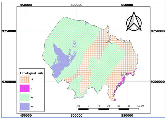
Figure 3.
The geology of the Kimbiji aquifer.
3. Materials and Methods
3.1. The Modified Soil Moisture Balance Method Coupled with Curve Number for Recharge Assessment
Natural groundwater recharge estimation in this study was carried out using the Modified Soil Moisture Balance Method (MSMB), which was originally developed in the 1940s by Thornthwaite [23], and later revised by Thornthwaite and Mather [24]. The MSMB method capitalizes on the concept of water balance of the unsaturated zone, keeping track of the accumulated potential water loss (APWL) and the amount of water stored in the soil (SB) [25,26,27,28]. As soil moisture diminishes, water in the soil becomes more and more tightly bound to the soil particles and it is, therefore, difficult to be removed.
Different parameters of the soil moisture budget were computed using the Thornthwaite Water Balance software as applied elsewhere [29] utilizing the PET (calculated from daily maximum and minimum temperature) and rainfall obtained from the gauging stations and the Tanzania Meteorological Agency (TMA). The water balance referred to in this method is basically the balance between the incoming water from precipitation and the outflow of water by evapotranspiration [30,31]. Calculations to determine SB and APWL were performed for each day using daily precipitation (P) and potential evapotranspiration (PET) data. The accumulated potential water loss (APWL) represents the accumulated rainfall deficits and increases with increasing difference between PET and precipitation (minus runoff). Principally, natural groundwater recharge is only possible when precipitation minus runoff is larger than the PET, and it usually happens during the rainy season. This scenario is represented by Equation (1).
Nevertheless, this scenario does not ensure a spontaneous recharge, as the amount of water that is left after subtracting the PET from the rainfall minus runoff will first be held by the soil. At a certain point, the amount of water held by the soil (SB) will exceed its maximum threshold called the field capacity (CAP). The surplus of water after reaching the field capacity recharges the aquifer. At this point, the actual evapotranspiration (AET) is equal to the PET. This scenario is represented by Equation (2).
During the dry season, PET is normally higher than the amount of precipitation minus runoff. In this case, there is not enough water available to reach or even surpass the PET. Thus, the actual evapotranspiration will be infinitesimally smaller than the PET. This situation is represented in Equation (3).
Understanding the concept of field capacity is very instrumental in the soil moisture balance method. It denotes an upper limit of moisture content a soil can hold against the pull of gravity. Soil water holding capacity is affected by soil type as well as vegetation type (rooting depth), and it is usually the product of water content at field capacity and average rooting depth. In a conceptual sense, groundwater recharge can commence when the moisture content exceeds field capacity [32,33]. It is, therefore, ostensible that no rainfall-based (natural) recharge will happen in the dry season because the soil water content decreases logarithmically and reaches its minimum at the permanent wilting point (PWP) during the dry season. According to Raes et al. [34], PWP is the soil water content at which plants can no longer extract water and will wilt permanently. The difference between the water at field capacity and the water at permanent wilting point, multiplied by the rooting depth is referred to as the plant available water (PAW) [34]. PAW was, therefore, estimated, as shown in Equation (4).
where Dr is the rooting depth.
A deeper rooting zone means that there is a larger volume of water stored in the soil zone and, therefore, a reduced amount of water going to the groundwater reservoir as recharge. Arguably, an area with thin soils and low values of PAW (<200 mm) should be used, while in areas with deep soils, medium to high values of PAW (>200 mm) should be used [30]. To that effect, a PAW of 250 for the Kimbiji aquifer was used due to their relatively deep soils, while a PAW of 100 was used for the Singida aquifer. This was guided by the type of soils, vegetation, and amount of annual rainfall received in each study area, which is reflected in the plant available water.
3.2. Runoff Estimation Using the Modified Curve Number Method
Runoff is invariably one of the most important parameters for natural groundwater recharge estimation using the soil moisture balance method. The generation of runoff in a landscape is controlled by the interaction of precipitation with the topography, land use, and soil properties of the land surface as provided for by Patil et al. [35]. The SMBM converts rainfall to surface runoff using curve number that is derived from basin characteristics and 5-day antecedent rainfall. Although this method was previously criticized by other researchers [36,37] because the amount of generated runoff does not take into account the rainfall intensity nor the slope factor, to date, the method is widely accepted and used by scientists in different domains for estimation of runoff [27,30,31,38]. This study has minimized the shortfalls of the method, including offsetting the two aforementioned shortcomings by considering the two factors in the modified soil moisture balance method. Surface runoff, which is the fraction of precipitation that flows on impervious surfaces or over the land surface was subtracted from the precipitation to compute the residual amount of precipitation that participates into the further steps of the soil moisture balance process.
Generally, the runoff results from the interaction of precipitation with the topography, land use, and soil properties of the land surface under study, as opined by Patil et al. [35]. In the process of estimating surface runoff, curve number is such an important parameter. However, in the determination of a curve number for the two study areas, there are a number of factors to be considered that are key and greatly contribute to the derivation of the curve number of any landscape. These are the hydrologic conditions of a basin, hydrological soil groups found in the basin, antecedent soil moisture conditions, and land cover types. Each of these factors are described in detail.
3.3. Land Use Land Cover (LULC) Classification
Land use land cover (LULC) classification followed a detailed understanding of the spatial extents and geographical delineations of the two study areas. Clear and cloudless satellite images were downloaded from the USGS earth explorer sites, covering path 166 and row 65 for the Kimbiji aquifer and path 169 and row 63 for the Singida aquifer. In order to carry out LULC classification using the semiautomatic classification plugin in QGIS, the knowledge of specific areas of the image and what underlying values belong to which class was critically important. Satellite images from Landsat Thematic Mapper (TM), which included 1995, 1997, 2005, and 2008, and Landsat 8 Operational Land Imager-Thermal Infrared Sensor (OLI-TIRS) for 2016 and 2018 were downloaded from the Global Visualization (GloVis) site (https://glovis.usgs.gov) and the Earth Explorer (https://earthexplorer.usgs.gov/) site of the United States Geological Survey (USGS), and they were subjected to digital image processing.
The choice of the number of LULC classes was based on the requirements of and purpose of this study. The major focus was choosing images that would serve a purpose for estimating curve numbers and recharge thereafter. This was also emphasized in the choice of LULC classes. Eight major LULC classes were chosen for mapping in each of the two study areas. After the preparation of classification scheme, the maximum likelihood classification technique in the Semiautomatic Classification Plugin (SCP) in QGIS was adopted for LULC mapping for all the six images, three for each study area. The magnitude of change (MC), (Equation (5)), the percentage of change (PC), (Equation (6)), and the annual rate of change (ARC) (Equation (7)) for each LULC class in the two study areas for three different time spans were calculated as shown in the respective equations.
where Ai is the class area (km2) at the initial time, Af is the class area (km2) at the final time, and n is the number of years of the respective time period where land cover change analysis has been carried out.
3.4. Hydrological Soil Groups
Soil properties significantly influence the amount of runoff in an area. The influence of both the soil’s surface condition (infiltration rate) and its horizon (transmission rate) are key in determining the potential of any soil to groundwater recharge. The two properties that indicate a soil’s runoff potential form the qualitative basis of the classification of all soils into four hydrologic soil groups, as summarized in Table 1.

Table 1.
Characterization of Hydrological Soil Groups.
3.5. Antecedent Moisture Condition
The soil moisture condition in a basin before runoff occurs is another important factor influencing the final CN value, and subsequent groundwater recharge. Runoff is affected by the soil moisture before a rainfall event. This is known as antecedent moisture condition (AMC). In the modified soil moisture balance method with Curve number, the AMC is categorized into three classes (Table 2). The classes are based on the 5-day antecedent rainfall, which is the accumulated total rainfall preceding the runoff under consideration. AMC is an indicator of the wetness and availability of moisture content of soil storage prior to a storm rainfall event [39,40].
Table 2.
Group of Antecedent soil moisture classes.
The CN method distinguishes the dormant and the growing season in order to highlight the differences in actual evapotranspiration between the two seasons. The values of CN used in this study, as proposed previously [41], are valid for an average relationship where initial abstraction, Ia = 0.2S, and for average antecedent soil moisture condition (AMC II), S being the potential maximum retention. Moreover, the curve number, as determined in this study, was termed CN II, which is derived from AMC II (average soil moisture condition). The other moisture conditions are AMC I (dry) and AMC III (moist), which were not used in this study. The application of the three AMC classes is hugely determined by the rainfall intensity of the previous 5 days, known as 5-day antecedent rainfall and season.
To determine the appropriate CN value, a table relating the value of CN to land use/cover type, land cover treatment and/or practice, hydrological condition, and hydrological soil group was used in this study (Table 3). With the aid of those tables, coupled with succinct field campaigns and ground truthing, the curve numbers for the two study areas were determined. A calculation of the weighted average, CN, taking into account the areas they occupy, utilizing the data given in Table 3, was carried out using Equation (8).
where CNi—curves number in per unit, Ai—Area (km2) and A—the total area of the study area. The data in Table 3 facilitated the estimation of the mean weighted curve number.
Table 3.
Curve numbers for various land covers from the study areas as adopted from previous studies [17,30,41].
3.6. Estimation of Weighted Curve Numbers for Kimbiji and Singida Aquifers
The two Equations (9) and (10) were used to calculate weighted curve numbers for the Kimbiji aquifer (CNKIMB) and the Singida aquifer (CNSING), respectively. The letters CN and A stand for curve number and area, respectively. The subscripts abbreviate the respective land covers, where f is forest, w is woodland, bs denotes bushland, and gs stands for grassland. Further, wa represents water, we is for wetland, cl connotes cultivated land, and ba is for built-up area.
Equation (11) underpins the prediction of runoff from the amount of rainfall, using a shape factor (S), called the potential maximum retention. The shape factor combines the effects of soil, vegetation, land use, and antecedent soil moisture (i.e., soil moisture prior to a rainfall event). The rule of thumb is, at the start of the rainfall event, water will be intercepted by land covers/crops, stored in small depressions, and infiltrated in the soil as initial abstraction (Ia). After runoff has been generated, some of the additional precipitation will infiltrate, forming the actual retention (F). With increasing precipitation, the actual retention eventually reaches a maximum value that is the potential maximum retention (S), as depicted in Equation (12).
However, if , then it follows that RO = 0, where RO is the runoff (mm), P is the precipitation (mm), Ia is the initial abstraction (mm), S is the potential maximum retention (mm), and Ia = 0.2S.
Therefore,
If the parameter S is known, CN can be calculated from Equation (13).
where CN is a dimensionless parameter known as Curve number, whose value ranges from 0 to 100.
Curve number designates the runoff response characteristics of an area that depends on the land use type, land treatment, hydrological condition, hydrological soil group, and antecedent soil moisture of the area. Other studies [42] described hydrologic condition as the effects of cover type and treatment on infiltration and runoff and is generally estimated from density of plant and residue cover on sample areas. Good hydrologic condition indicates that the soil usually has a low runoff potential for that specific hydrologic soil group, cover type, and treatment. Antecedent moisture is considered to be low when there has been little preceding rainfall and high when there has been considerable preceding rainfall prior to the modelled rainfall event. For modeling purposes, in this study, the AMC II, which is essentially an average moisture condition, was considered. It is practically straightforward to estimate the parameter S using Equation (14) when the CN is known.
Therefore, runoff was estimated using Equation (15), which is embedded in the recharge calculation tool using the modified soil moisture balance method that is coupled with curve number.
3.7. Potential Evapotranspiration
Potential evapotranspiration was calculated using the Penman–Monteith (PM) method and the Hargreaves–Samani (HS) method. The combination of the two methods was chosen to assess the significance of the claims on PET overestimation and underestimation [17,30]. Reportedly, the two temperature-based PET methods (i.e., PM and HS) are as reliable as physically based methods [43,44]. Therefore, PET calculated using the Penman–Monteith (PM) method was compared with PET that was calculated using the Hargreaves–Samani (HS) method.
The Penman–Monteith method uses Equation (16), which is embedded in the reference evapotranspiration (ETo) program developed by the United Nation’s Food and Agricultural Organization (FAO). This program has proven to be the best method to estimate potential evapotranspiration in data scarce environments such as Tanzania [45]. The method does not require a wide variety of weather data, which are basically not always available in many parts of the world [30]. ETo program requires meteorological data inputs, mainly daily maximum and minimum temperature as well as the climatic station characteristics such as geographical coordinates (latitude and longitudes) of the station, elevation, topographic attributes, station descriptions, including the country where the station is found. Of equal importance are the characteristics of wind systems in the study area. After providing all the aforementioned inputs into the ETo program, the other variables shown in Equation (16) are numerically estimated. As varies only slightly over normal temperature ranges, a single value of 2.45 MJ kg−1 is taken in the simplification of the FAO Penman–Monteith equation. This is the latent heat for an air temperature of about 20 °C.
where PETPM is the evapotranspiration (mm day−1) calculated using the Penman–Monteith equation, Rn is the net radiation at the crop surface (MJ m−2 day−1), G is the soil heat flux density (MJ m−2 day−1), T is the mean daily air temperature at 2 m height (°C), U2 is the wind speed at 2 m height (m s−1), es is the saturation vapor pressure (kPa), ea is the actual vapor pressure (kPa), es − ea is the saturation vapor pressure deficit (kPa), is the slope vapor pressure curve (kPa °C−1), and is the psychrometric constant (kPa °C−1).
The other method was the temperature-based Hargreaves–Samani (HS) approach. Numerically, the PET using Hargreaves–Samani approach was calculated as shown in Equation (17) and its requisite requirements are described thereafter. Arguably, no local correction is required for windy locations for the Hargreaves–Samani equation [46]. Moreover, it was recommended using an empirical coefficient equal to 0.0020 for non-windy locations such as the Kimbiji aquifer instead of the original value (0.0023) proposed by Hargreaves and Samani [47], which, in this study, was applied in the Singida semi-arid aquifer. Equation (17) represents the HS method of temperature-dependent PET method used in this study.
where PETHS is the daily PET in mm/day calculated using the Hargreaves–Samani method; Ra is the extraterrestrial radiation in mm/day; Tmax and Tmin are daily maximum and minimum air temperature in °C, respectively; kRS is the empirical radiation adjustment coefficient (0.0023) for the Kimbiji and Singida aquifers; HE is the empirical Hargreaves exponent, and the value is set to 0.5 in the two study areas; and HT is the empirical temperature coefficient, and the value is set to 17.8.
The daily rainfall and PET data were arranged into hydrologic years, starting at the beginning of the short rainy season, and terminating at the dry season after the long rainy season (October to November) for the bimodal Kimbiji aquifer and November to October for the unimodal Singida aquifer. Organizing data in a hydrological year has the advantage of facilitating the computation of the change in soil moisture storage at the beginning of the hydrologic year, because the soil moisture storage at the end of the dry season is normally considered to be completely depleted. Additionally, the concept of hydrologic year reflects the natural climatic reality in the sense that it commences with the start of the period of soil moisture replenishment, goes through the period of maximum groundwater recharge, if any, and culminates with the season of maximum soil moisture utilization [30,45]. Moreover, the Aridity index (AI), which is the ratio of Rainfall and Potential Evapotranspiration, was also used to characterize the study area. According to previous studies [21], when AI < 0.05, that indicates hyper-aridity. The area is in arid conditions if 0.05 < AI < 0.2. Moreover, 0.2AI < 0.5 signals semi-arid conditions. Dry sub-humid and humid conditions are represented by 0.5 < AI < 0.65 and 0.65 < AI < 0.75, respectively. Hyper-humidity occurs when AI > 0.75.
3.8. Assessing the Influence of El Nino and the Southern Oscillation on Rainfall and Recharge Using the Southern Oscillation Index
The Southern Oscillation refers to changes in Sea-Level Air pressure patterns in the Southern Ocean between TAHITI and DARWIN. During El Niño conditions, the average air pressure is higher at DARWIN than at TAHITI. The Southern Oscillation Index (SOI) was calculated from the monthly fluctuations in the air pressure difference between Tahiti and Darwin using the Australian Bureau of Meteorology method called the Troup SOI. The Troup SOI is the standardized anomaly of the Mean Sea Level Pressure difference between Tahiti and Darwin. Based on the above method, SOI was calculated as shown in Equation (18).
where
- Pdiff = [Average Tahiti Mean Sea Level Pressure (MSLP) for the month] − [Average Darwin Mean Sea Level Pressure (MSLP) for the month];
- Pdiffav = Long term average of Pressure difference (Pdiff) for the month in question;
- SD (Pdiff) = Long term standard deviation of Pdiff for the month in question.
4. Results
4.1. Land Cover Change Assessment
The LULC classification results show a significant decrease in forested land and woodland in the Kimbiji aquifer, while there has been a noticeable increase in grassland and cultivated areas (Table 4), possibly as a result of forest and woodland degradation. Areas covered by water bodies have decreased steadily from almost 1 to 0.2% from 1997 to 2016 in the Kimbiji aquifer. This went hand in hand with the decrease in wetland areas from 2% in 1997 to 0.2% in 2016. This signifies that during that period, 80% of the areas covered by water have been changed to another land cover/use, while 90% of the wetland areas were converted into other land covers as well. The tremendous expansion of agricultural activities from 1997 to 2016 (0.6 to 25%) in the Kimbiji study area, and the growth of urban areas, 1.5% in 1997 to 4% in 2016, can ostensibly be attributed to the observed decrease in other land covers, as shown in Table 4. The bushland maintained its equilibrium level in 2016 after an observed increase in 2008. Cultivated land has increased, as has the built-up area in the Kimbiji aquifer (Table 4).
Table 4.
Temporal land cover change matrix for the Kimbiji aquifer.
While woodland, forests, and wetland have been decreasing tremendously in the Singida aquifer, the cultivated land increased by 200% from 1997 to 2018. The growth of the built-up area was almost constant (Table 5), increasing by 0.01% from 1997 to 2018. The decrease in forests and wetlands can be unwittingly attributed to the expansion of agricultural activities. Grasslands and bushlands have experienced some twisting dynamics, increasing from 1997 to 2005, and decreasing by 2018. The bushland was observed to decrease in 2018 but it did not reach the same level as of 1997 as it was the case for the Kimbiji aquifer. In the Singida aquifer, the cultivated land is most likely responsible for the conversion of other land covers such as forests, woodlands, bushes, and grasslands. The most enthralling scenario about the bushland in this study is that there has been an increase and a decrease afterwards in the two study areas. The factors for this observed similarity are most likely the same.
Table 5.
Temporal land cover change matrix for the Singida aquifer.
4.2. Assessment of the Magnitude and Annual Rate of Land Cover Changes
The assessment of the magnitude and annual rate of land cover changes revealed negative and positive annual rates of land cover changes in both study areas. In the Kimbiji aquifer, for instance, the overall annual rate of change of forest cover was approximately 19 km2/year, with the highest annual rate of forest cover change (24.2 km2/year) occurring between 1997 and 2008 (Table 6). Forest cover dropped between 2008 and 2016, registering only 9.1 km2 per year (Table 6). The biggest land cover change in the Kimbiji aquifer between 1997 and 2016 was a gain of cultivated land by almost four times, followed by built-up areas (−170%) and the grassland (−50%). The other land covers in the Kimbiji aquifer had emaciated due to various reasons, with woodland and forests being at the epicenter of land cover losses. In the Singida aquifer, as it was for the Kimbiji aquifer, cultivated land increased by 2588.2 km2 per year between 1997 and 2018 (Table 7), while the loss of woodland was the highest of all the land covers in the Singida aquifer. Generally, there was a gain in the built-up area (0.9 km2 per year), area covered by water, and bushes also increased by almost 29 km2 per year. The other land covers (wetland, forest, woodland, and grassland) declined per year, as shown in Table 7 for the Singida aquifer. The spatiotemporal variation of land covers for the Kimbiji and Singida aquifers is shown in Figure 4 (A = LULC for 1997 in Singida, B = LULC for 2005 in Singida, C = LULC for 2018 in Singida, D = LULC for 1997 in Kimbiji, E = LULC for 2008 in Kimbiji, F = LULC for 2016 in Kimbiji).
Table 6.
The magnitude of change, percentage of change, and the annual rate of change for land cover classes in the Kimbiji aquifer.
Table 7.
The magnitude of change, percentage of change, and the annual rate of change for land cover classes in the Singida aquifer.
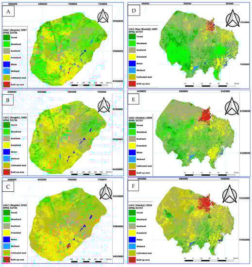
Figure 4.
Land cover maps for the Kimbiji and Singida aquifers. (A) LULC for 1997 in Singida, (B) LULC for 2005 in Singida, (C) LULC for 2018 in Sin-gida, (D) LULC for 1997 in Kimbiji, (E) LULC for 2008 in Kimbiji, (F) LULC for 2016 in Kimbiji.
4.3. Land Cover Classification Accuracy Assessment
The overall accuracies for 1997 were 87.3 and 85.7% for Kimbiji and Singida, respectively (Table 8). For 2008 and 2016 in the Kimbiji aquifer, the overall accuracy was 88.0 and 86.5%, respectively, while for 2005 and 2018in Singida, the accuracies were 89.2 and 93.6%, respectively (Table 8). The overall accuracy of the six different maps represents the percentage of correctly classified pixels as reported in other previous studies [48,49,50]. The Kappa coefficients range between 0.81 to 0.89 for the Kimbiji aquifer and 0.79 to 0.86 for the Singida aquifer, indicating a perfect agreement between the classified land covers and the reference sites (ground control points). Reportedly, a minimum kappa threshold of 0.61 is an acceptable agreement threshold [51]. The land cover classification results in the study areas are in a perfect agreement.
Table 8.
Accuracy Assessment parameters for land cover classification results.
4.4. The Weighted Curve Numbers for the Kimbiji and Singida Aquifers
Table 9 presents the weighted curve number results for the two study areas. The curve number for the Kimbiji aquifer is relatively smaller than the Singida aquifer, indicating a higher runoff potential in the Singida aquifer than the Kimbiji aquifer. The curve number in the Singida aquifer was observed to decrease between 1997 and 2005, then it slightly increased in 2018. Comparatively, there has been a quasi-stable CN in the Singida aquifer (74.2 in 1997, 73.64 in 2005, and 73.87 in 2018) but a steadily increasing CN for the Kimbiji aquifer (66.69 in 1997, 69.08 in 2008, and 71.42 in 2016). It was also observed that the forest cover in the Singida aquifer has a higher curve number than the forest cover in the Kimbiji aquifer. This is due to the difference in the agroclimatological conditions that are considered for choosing a tabulated CN of a particular area. The area covered by water for the Kimbiji aquifer, mainly represented by rivers, has a relatively lower curve number as compared to the same class in the Singida aquifer. This is because the water bodies in the Singida aquifer are mainly lakes, while in the Kimbiji aquifer, the water bodies are mainly represented by rivers. Grassland for the Kimbiji aquifer has a relatively low runoff potential as compared to the same class in the Singida aquifer. This is again attributed to the difference in climate between the two study areas. The drier the area is, the higher the runoff potential is given that other factors remain the same.
Table 9.
Land cover related average and weighted curve number for the Kimbiji and Singida Aquifers.
The difference in the average curve number between dry and humid environments has been observed, especially for forests, woodlands, and grasslands (Table 9). The contribution of cultivated land to the weighted curve number kept on increasing due to an increase in the size of land under agricultural activities over time in the two study areas. It increased by three folds in the Kimbiji aquifer, while it doubled in the Singida aquifer (See Table 9). However, the growth of built-up areas and their contribution to the curve number is fascinatingly exponential, despite the small size of the land under settlement. The contribution of built-up areas in the two aquifers was relatively meager due to the fairly small size of the land as compared to the size of the area under study. However, the runoff potential is higher in the Kimbiji aquifer than it is in the Singida aquifer. An insignificant change in the curve number for the Singida aquifer was observed, although there has been some noticeable land cover dynamics from 1997 to 2018, as depicted in the land cover maps. As for the Kimbiji aquifer, there has been an increase in the curve number (Table 9), which signifies a concurrent change in land covers, which hugely influence runoff in the study area.
4.5. Potential Evapotranspiration, Rainfall, Runoff, Groundwater Recharge, and Aridity Indices
In Table 10 and Table 11, the results for rainfall, net rainfall, potential evapotranspiration, runoff, groundwater recharge, and aridity indices are presented for the different hydrological years for Kimbiji and Singida aquifers, respectively. The recharge and aridity indices correspond with the PET values calculated using the two temperature-dependent methods as explained earlier on. For the Kimbiji aquifer, the PET values obtained using Penman–Monteith (PM) for the 1996/1997, 2007/2008 and 2015/2016 hydrological years were 1156.5, 1079.5, and 1143.9 mm/year, respectively, while for the Hargreaves–Samani (HS) method, the PET was found to be 1046.1, 1138.3, and 1204.4 mm/year for the 1996/1997, 2007/2008, and 2015/2016 hydrological years, respectively. For the Singida aquifer, the PM PET method resulted in 2083.3, 2053.6, and 1875.4 mm/year for the 1996/1997, 2004/2005 and 2017/2018 hydrological years, respectively. The HS method produced relatively lower PET values for the Singida aquifer, which are 1839.4, 1814.7, and 1710.2 mm/year for the 1996/1997, 2004/2005, and 2017/2018 hydrological years, respectively.
Table 10.
Rainfall, PET, and Recharge for 1996/1997, 2004/2005, and 2017/2018 hydrological years for the Kimbiji Aquifer.
Table 11.
Rainfall, PET, and Recharge for 1996/1997, 2004/2005, and 2017/2018 hydrological years for the Singida Aquifer.
It was realized that the HS method overestimated the PET in the Kimbiji humid aquifer except for the 1996/1997 hydrological year (Table 10). This is possibly due to the excessive rainfall received in that period due to the influence of the ENSO. Excessive rainfall lowers surface temperatures (maximum and minimum), which ultimately lowers the rates of evaporation and transpiration. This explains the high sensitivity of the HS method to changes in the maximum and minimum temperatures as compared to the PM method. In the Singida aquifer, the HS method underestimated the PET, while the PM overestimated it. Nevertheless, the difference in the calculated PET between the two methods is significantly higher in the Singida semi-arid aquifer than the observed difference in the Kimbiji aquifer.
4.6. Groundwater Recharge Response to Climate and Land Cover Dynamics
The graphing of the PET, rainfall, runoff, recharge, and net rainfall (Figure 5) revealed that the PET calculated using HS method was more realistic than the PET derived from the PM method. The PM-based PET graph was observed to be above the rainfall and net rainfall graphs throughout the year, even during the rainfall season. This translates into a complete lack of natural recharge due to net rainfall being negative throughout the year. This is quite misleading because during rainfall, the PET values are lowered, and the net rainfall becomes positive. progressively leading to groundwater recharge. This has been demonstrated by the HS PET-based graphs. To that effect and for the sake of consistency, the HS-based PET values were adopted for the two study areas, disregarding the PM-based PET for recharge estimation.
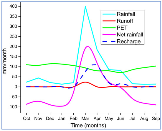
Figure 5.
A 1996/1997 hydrological year graph of rainfall, runoff, PET, net rainfall, and aridity index in the Kimbiji aquifer.
Despite the variability in climate from 1997 to 2018, the aridity indices have confirmed that the Kimbiji aquifer is in a humid area, while the Singida aquifer is found in a semi-arid area. The indices in the Kimbiji aquifer were found to range between 0.7 and 0.9 (Table 10), while in the Singida aquifer, they range between 0.3 and 0.45 (Table 11), despite the overestimation of the PET using the PM method. According to previous studies [52,53], these indices are within the humid and semi-arid areas for the Kimbiji and Singida aquifers, respectively.
Figure 5 is a graph for the 1996/1997 hydrological year for the Kimbiji aquifer, which shows a time lag between rainfall and recharge. The response of runoff is spontaneous and directly related to the observed rainfall event. While peak rainfall was observed in March, the water table fluctuation as a result of the March rainfall was realized in April. In the rainy season, the PET was also seen to decrease because of the reduced surface temperatures. This can also be observed in the short rainfall season between October and December (Figure 5), where net rainfall, rainfall, and the PET responded to it. There was no discernible response of the aquifer in terms of natural groundwater recharge to the short rainfall season, nor did the runoff change.
For the 2007/2008 hydrological year (Figure 6), the time lag diminished as the peaks of rainfall, net rainfall, and recharge are all seen in April. Runoff responded to short rainfall event, unlike in the 1996/1997 hydrological year. Where rainfall exceeded the PET, the PET graph fell below the rainfall graph, while the opposite could be observed when the PET was higher than rainfall. From Figure 6, it can be seen that in the 2007/2008 hydrological year, there was a prolonged dry spell between December and February, which could be the reason behind the aforesaid soil moisture deficit towards the long rainfall season in the 2007/2008 hydrological year. The 2015/2016 hydrological year graph (Figure 7) portrays a discernible response of runoff to the short rainfall event between October and December with a dwarfed runoff hydrograph in the long rainfall season between March and May. However, recharge was relatively more pronounced than runoff in the long rainfall season, suggesting that in the 2015/2016 hydrological year, soil moisture was relatively higher towards the long rainfall season than in the 2007/2008 hydrological year.
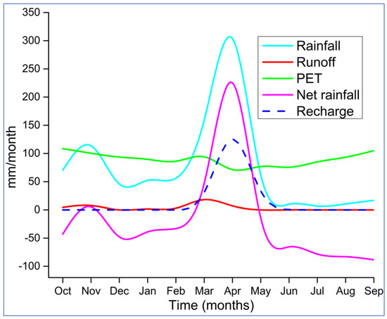
Figure 6.
A 2007/2008 hydrological year graph of rainfall, runoff, PET, net rainfall, and aridity index in the Kimbiji aquifer.
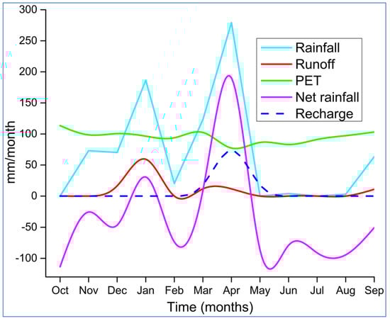
Figure 7.
A 2015/2016 hydrological year graph of rainfall, runoff, PET, net rainfall, and aridity index in the Kimbiji aquifer.
Figure 8 represents the 1996/1997 hydrological year graph for the Singida aquifer. Unlike other hydrological years, the 1996/1997 hydrological year showed a somewhat different trend of the response of recharge to rainfall and net rainfall. The peak rainfall was observed in December, as were the peaks of recharge and net rainfall. This is directly linked to the occurrence of the ENSO, where its major impact in Tanzania is above normal rainfall. This can also be justified from Table 11, where the Singida aquifer received abnormally higher rainfall (i.e., 831 mm/year) in the 1996/1997 hydrological year.
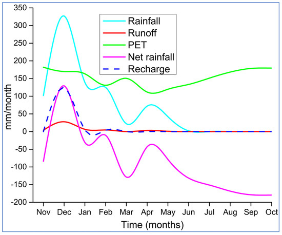
Figure 8.
A 1996/1997 hydrological year graph of rainfall, runoff, PET, net rainfall, and aridity index in the Singida aquifer.
A time lag in natural groundwater recharge was quite ostensible in the 2005/2006 hydrological year for the Singida aquifer. A quasi-bimodal season has also been observed in this hydrological year (Figure 9), suggesting a break in the rainfall season between January and March. This is typical of the areas that receive one long rainfall season (unimodal), where a dry spell in between the rainfall season happens. Due to a pronounced dry spell, soil moisture deficit was high to the extent of suppressing the runoff.
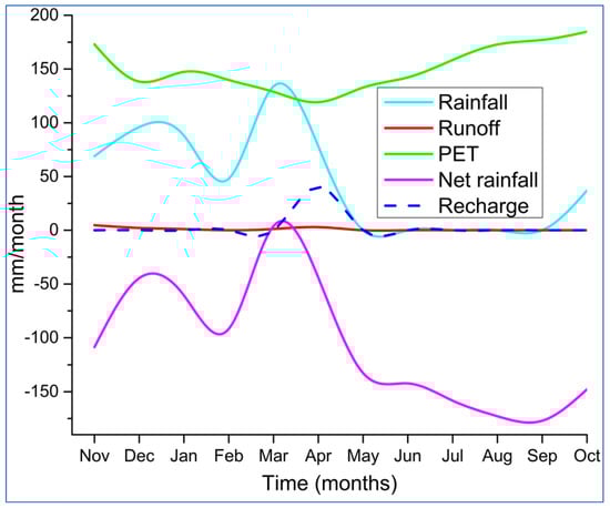
Figure 9.
A 2005/2006 hydrological year graph of rainfall, runoff, PET, net rainfall, and aridity index in the Singida aquifer.
The 2017/2018 hydrological year portrays (Figure 10) a quasi-bimodal rainfall season in the Singida aquifer. This is because there seemed to be an extended dry spell in February 2017 that resulted into two separate peaks of rainfall events. This is normal for years that receive a relatively low amount of rainfall. The observed scenario is supported by the lack of ENSO teleconnections (Figure 11) where there was no sustained negative SOI, which signals ENSO-related rainfall in the East African region, and Tanzania in particular. Runoff is observed to decrease with decreasing rainfall in the Singida aquifer. Despite this trend, recharge was also decreasing.
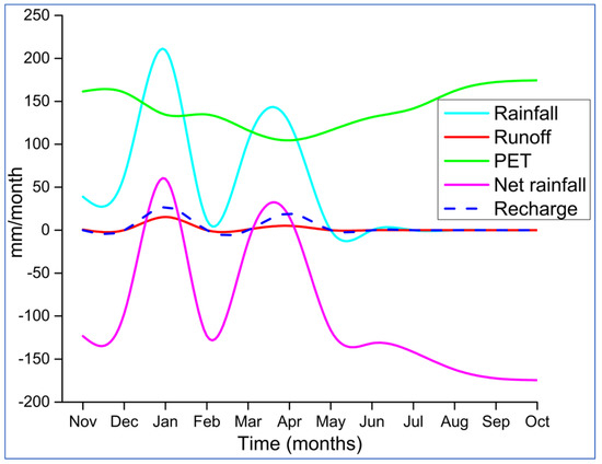
Figure 10.
A 2017/2018 hydrological year graph of rainfall, runoff, PET, net rainfall, and aridity index in the Singida aquifer.
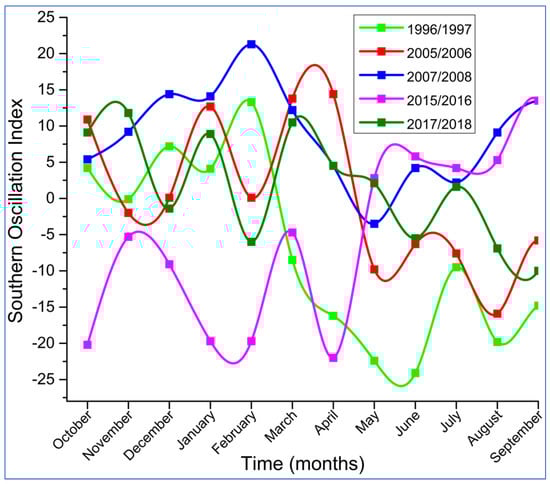
Figure 11.
The graph of Southern Oscillation Index for depicting the influence of El Nino and the Southern oscillation on rainfall.
In this study, it has been revealed that climate teleconnection through the Southern Oscillation Index is related to rainfall anomalies observed in the two study areas. During El Niño events, rainfall and groundwater recharge increased. The response of rainfall, and ultimately groundwater recharge, disregards the difference in climate and geology between the Kimbiji, humid, Neogene sedimentary aquifer and the Singida, semi-arid fractured, crystalline basement aquifer. The 1996/1997 and 2015/2016 hydrological years experienced sustained negative ISO values from March to December in 1997, October to December 2015, and January to April in 2016 (Figure 11). The 2007/2008 hydrological year had little signs of the ENSO due to more sustained positive SOI values as compared to the rest of the years. The 1996/1997 and 2005/2006 hydrological years were observed to be under the influence of the ENSO more than the other hydrological years. This phenomenon had a noticeable impact on groundwater recharge.
5. Discussion
There is an observed concomitant decrease in forests, woodlands, and wetlands, while areas under cultivation and human settlements tended to increase in size over time in the two study areas. The observed trend has also been reported previously [16]. The decrease in forested land in the Kimbiji aquifer can be more attributed to human settlements, while in the Singida aquifer, agricultural land has claimed a huge chank of the forest land and woodlands as explained by the annual rate of change of forests and woodlands in the two study areas. The decrease in wetlands and grassland at the expense of increasing the agricultural land has also been reported elsewhere [54]. The expansion of urban areas at the expense of agricultural land was also reported in previous studies, highlighting some potential impacts of such land cover changes on water resources [55,56,57,58].
Reportedly, the absence of or the weakness of institutions, including inept accountability, are some of the factors that encourage the encroachment of forests by either the clearance of vegetation cover for agricultural expansion or by cutting trees for gathering firewood [59,60]. Charcoal making for cooking and business can as well be attributed to the loss of forest cover in the two study areas as discussed previously [55,57]. Forests are also affected by forest fires, which cause excessive forest and woodland degradation due to anthropogenic activities [60]. Other researchers [55,56,57] reported that the decrease in forest and woodland can be associated with the conversion of forest land to built-up areas (in the Kimbiji aquifer) and farmland (in the Singida aquifer).
The study has revealed that natural groundwater recharge is affected by the dynamics of land covers as well as climate despite the differences in climate and geology. There is a decreasing trend of recharge corresponding with a decreasing trend of rainfall. Moreover, an increasing trend of curve number has been observed in the Kimbiji aquifer, corresponding to the increase in runoff. This also affects groundwater recharge negatively. The PET has also been observed to increase in the two aquifers regardless of their difference in climate. Therefore, the increase in the PET and the curve number justifies the progressive decrease in groundwater recharge with time, representing climate and landcover factors, respectively. Nevertheless, the effect of climate variability to groundwater recharge is more prominent in the Singida aquifer, while in the Kimbiji, a combined effect of climate variability and land cover changes to groundwater recharge has been observed. In the Kimbiji aquifer, runoff is increasing steadily, while other parameters showed a similar trend as those of the Singida aquifer. Recharge kept on decreasing as a result of the increasing PET due to an increase in surface temperatures, both maximum and minimum. In the Singida aquifer, the weighted curve number stabilized with time, while recharge was observed to decrease. This enlightens on the influence of rainfall variability on groundwater recharge other than land cover changes in the dry-semi-arid Singida aquifer. This also informs of the presence of local recharge as an important component of groundwater flow systems in the semi-arid Singida aquifer.
Moreover, despite the dereference in climate and geology, groundwater recharge followed a positive trend as rainfall in the two study areas. This reiterates what was reported earlier on by Oke et al. [19]. This study has also proven that decreasing rainfall contributes to decreasing groundwater recharge, as pointed out by other researchers [9]. During the dry season, no rainfall surplus was observed, and it obeyed this rule of thumb that, ([P − Ro] − PET 0), and there was no groundwater recharge in all the two basins regardless of the difference in climate and geology. Groundwater recharge occurred whenever rainfall minus runoff was larger than the PET, obeying the equation ([P − Ro] − PET >0), as discussed previously [17,30,45], and it usually happened during the rainy season. This is because, during the rainy season, the net rainfall is usually positive. This observation confirms the fact that there is a local flow component in each of the two study areas albeit different in magnitude.
The 1996/1997 and 2005/2006 hydrological years were observed to be under the influence of the ENSO more than the other hydrological years. This phenomenon had a noticeable impact on groundwater recharge. It has been noticed that the climate of the two basins, albeit different, is modulated by the El Niño-Southern Oscillation (ENSO) as it has been observed in previous related studies [61]. The ENSO has a significant influence on groundwater recharge in both humid and semi-arid areas as it has on streamflow and flooding, as pointed out previously [62]. The most recent strong El Niño of 1997/1998 has been reflected in the magnitude of annual rainfall as well as the annual groundwater recharge in the two basins. The moderate La Niña that developed slowly during 2007 could possibly be associated with reduced rainfall as well as a decrease in recharge in the two basins. Despite their difference in climate, the response to episodic climate systems (the ENSO in particular) has been noticeable. The ENSO’s contribution to the observed groundwater recharge cannot be ignored in the two aquifers, despite their contrast in climate and geology.
In addition, it was revealed that in the Kimbiji aquifer, runoff increased with decreasing rainfall for the 1996/1997, 2007/2008, and 2015/2016 hydrological years. In the Singida aquifer, runoff fluctuated with fluctuating rainfall. The 1996/1997 hydrological year in the Singida aquifer experienced high rainfall, attributable to the observed El Nino and the Southern Oscillation (ENSO) phenomenon. This resulted into almost 47 mm/year of run off. In the 2004/2005 hydrological year, runoff dropped tremendously to 12.2 mm/year, which reflects a tremendous drop in the annual rainfall in that year to 550 mm/year in the Singida aquifer. The fluctuation of recharge, apart from other factors, followed the fluctuation of the PET and rainfall.
The effect of urbanization on groundwater recharge has been revealed through urban growth in the Kimbiji aquifer, where a growth in built-up area resulted in an increase in the curve number. In the Singida aquifer, where urban growth was insignificant compared to other land covers, an insignificant increase in the curve number was shown. The findings of this study, which relate the response of land cover changes to an increase in surface runoff, which ultimately was found to affect groundwater recharge, are in line with what was reported previously [5,10,11,12,14,16,55,56,57]. Since surface runoff is linked to changes in land covers through the CN parameter, that change in some land covers had a huge impact on changes of runoff, and groundwater recharge thereof. The implication of land cover changes on water resources is quite discernible, albeit the concentration has been on surface water resources. The findings are also in line with what has been reported by other researchers [56,58], that various ecosystems are persistently being converted into agricultural land to feed the growing populations. Nevertheless, the impacts of such changes on water resources have been hugely ignored. This is likely to threaten the sustainability of water resources and socio-ecological systems at large.
The PM-based PET in the Singida aquifer showed that precipitation can no longer meet the evapotranspiration demand throughout the year. Thus, the unmet amount of water required by the evapotranspiration demand is increasingly taken from the soil moisture storage until it is fully exhausted. This does not represent reality, as local recharge is eminently happening in the Singida aquifer. The overestimation of the PET by various methods has been highlighted previously and the ensuing risk of generating incorrect recharge estimates thereof have been hinted too [30]. This study reiterates what has been reported previously on the possibility of underestimating and overestimating the PET, which is an important parameter in groundwater recharge estimation using soil moisture balance methods.
Time lags between rainfall and recharge are very prominent in the 2004/2005 and 2017/2018 hydrological years but less prominent in the 1996/1997 hydrological year in the Singida aquifer. Else, recharge in the other two hydrological years had responded to rainfall in the same month as the peak rainfall (April). For the Kimbiji aquifer, time lags between rainfall and recharge are not as prominent, except for the 1996/1997 hydrological year where rainfall peak was observed in March and the response of the aquifer to rainfall was observed in April. This observed difference in time lags between recharge and rainfall in the two aquifers explains the influence of geology and soil. The ENSO phenomenon in the 1996/1997 hydrological year offsets the influence in geology in the time lag between rainfall and recharge. This study has found that the two aquifers respond to rainfall events differently due to their difference in geology.
6. Conclusions
The implications of land cover changes and climate variability on natural groundwater recharge in the two aquifers with contrasting climate and geology have unveiled the hovering information with regard to the response to such perturbations. The effect of land cover change dynamics on groundwater recharge has been more prominent in the Kimbiji aquifer, while the effect of climate (rainfall and temperature) featured more prominently in the Singida semi-arid aquifer. This study also revealed that the same land cover can have a different runoff potential due to the difference in climate, geology, and soil properties. Such information goes missing in the recent and past literatures. This study has highlighted the difference in the curve number for similar land cover types owing to their difference in climate and geology.
The decline of certain land covers (forests) and increase in others (built-up areas), whose average curve numbers are relatively large, have contributed to the increase in surface runoff. This reduced the amount of rainwater that would otherwise infiltrate into the unsaturated zone, thereby recharging the aquifer, provided that the other hydrogeological conditions have been met.
The estimation of the PET using temperature-dependent methods resulted into a variation of the PET results, with HS overestimating the PET in the Kimbiji humid aquifer and underestimating it in the Singida semi-arid aquifer. The PM method overestimated the PET in the Singida aquifer, while underestimating it in the Kimbiji aquifer. Literally, the HS method is sensitive to changes in the maximum and minimum temperatures as compared to the PM method. PM underestimated the PET in the humid environment but overestimated the PET in the semi-arid environment, while HS overestimated the PET in the humid environment but underestimated the PET in the semi-arid environment. The PET overestimation by the HS method in the semi-arid environment was unsuitably unrealistic. Nevertheless, the overestimation of PET by the HS method in the Kimbiji aquifer was relatively smaller than the overestimation of PET by the PM method in the Singida aquifer. However, this does not directly translate into the PM PET method being less useful in all semi-arid areas because it requires long term studies with succinct longitudinal data collection to establish the empirical evidence on the suitability of the PM-PET based method in semi-arid areas.
As for this study, the HS approach seemed suitable, both in the humid Kimbiji aquifer and the semi-arid Singida aquifer. To that effect, this study uncovered the veiled scientific information on how basins with contrasting climates should be treated with regard to hydrological estimations and the calculation of runoff and groundwater recharge using the curve number as an indicator describing runoff response characteristics. Concerted care and attention must be paid to the choice of PET methods. The reported overestimation and underestimation in this study and other previous studies cannot be used as blueprints.
The ENSO phenomenon teleconnection with rainfall and groundwater recharge provided potentially useful information on how the difference in geology and climate cannot significantly feature in the response to El Nino teleconnections. The influence of the ENSO on time lags between rainfall and recharge has been observed and informs that, whenever there are ENSO teleconnections, time lags are offset, despite the difference in climate and geology. This is key for water resource management in the two basins with contrasting climate and geology. Harnessing the benefits accruing from episodic climate systems such as the ENSO in groundwater management is a foreseeable area of research. Moreover, prediction of the ENSO and its associated rainfall intensity would enable the ensuing natural groundwater recharge to be predicted.
Although general conclusions are drawn that groundwater recharge follows as positive a trend as rainfall [10], a more quantitative evaluation of the temporal variation of groundwater recharge due to the changing land covers and the implication of episodic weather events such as the ENSO is imperative to establish a more robust trend, which takes into account a number of variables other than rainfall alone. This is important for the management of groundwater resources in an optimal manner.
Author Contributions
Conceptualization, K.R.M.; methodology, K.R.M. and I.C.M.; software, K.R.M.; validation, I.C.M. and R.L.M.; formal analysis, K.R.M. and I.C.M.; investigation, K.R.M.; resources, K.R.M., I.C.M. and R.L.M.; data curation, K.R.M. and I.C.M.; writing—original draft preparation, K.R.M.; writing—review and editing, I.C.M., R.L.M. and K.R.M.; visualization, K.R.M. and I.C.M.; supervision, I.C.M. and R.L.M. All authors have read and agreed to the published version of the manuscript.
Funding
The research work from which this manuscript has been developed was funded by the Water, Infrastructure, and Sustainable Energy Futures (WISE FUTURES) Centre of Excellence based at the Nelson Mandela African Institution of Science and Technology (NM-AIST), Arusha-Tanzania.
Data Availability Statement
The data used to support the findings of this study are included in this article.
Acknowledgments
The authors wish to acknowledge the support of Water, Infrastructure, and Sustainable Energy Futures (WISE FUTURES) Centre of Excellence based at the Nelson Mandela African Institution of Science and Technology (NM-AIST), Arusha-Tanzania for the scholarship which catered for tuition fees, accommodation, meals, and partial research support. Additionally, the support from the Department of Geography and Environmental Studies at the Sokoine University of Agriculture is highly acknowledged for shouldering part of the PhD research costs through purchase of instruments and partial financial support to complement field activities. We are also highly indebted to staff of the Internal Drainage Basin (IDB) head office in Singida and the Wami/Ruvu basin head office in Morogoro for their support and open-handedness during field works and data provision.
Conflicts of Interest
Authors declare no conflict of interest with any organization, person, or a group of people that may impart bias of any kind in this work.
References
- Crosbie, R.; McCallum, J.; Walker, G.; Chiew, F. Episodic recharge and climate change in the Murray-Darling Basin, Australia. Hydrogeol. J. 2012, 20, 245–261. [Google Scholar] [CrossRef]
- Dowlatabadi, S.; Zomorodian, S.A. Conjunctive simulation of surface water and groundwater using SWAT and MODFLOW in Firoozabad watershed. KSCE J. Civ. Eng. 2016, 20, 485–496. [Google Scholar] [CrossRef]
- Polemio, M. Monitoring and management of karstic coastal groundwater in a changing environment (Southern Italy): A review of a regional experience. Water 2016, 8, 148. [Google Scholar] [CrossRef]
- Sharma, M.L. Measurement and prediction of natural groundwater recharge--an overview. J. Hydrol. 1986, 25, 49–56. [Google Scholar]
- Natkhin, M.; Dietrich, O.; Schäfer, M.P.; Lischeid, G. The effects of climate and changing land use on the discharge regime of a small catchment in Tanzania. Reg. Environ. Chang. 2013, 15, 1269–1280. [Google Scholar] [CrossRef]
- Bonan, G. Effects of land use on the climate of United States. Clim. Chang. 1997, 37, 449–486. [Google Scholar] [CrossRef]
- Pielke, R.A.; Avissar, R.; Raupach, M.; Dolman, H.; Zeng, X.; Denning, S. Interactions between the atmosphere and terrestrial ecosystems: Influence on weather and climate. Glob. Chang. Biol. 1998, 4, 461–475. [Google Scholar] [CrossRef]
- Sterling, S.M.; Ducharne, A.; Polcher, J. The impact of global land-cover change on the terrestrial water cycle. Nat. Clim. Chang. 2013, 3, 385–390. [Google Scholar] [CrossRef]
- Vazquez-Amábile, G.G.; Engel, B.A. Use of SWAT to Compute Groundwater Table Depth and Streamflow in the Muscatatuck River Watershed. Am. Soc. Agric. Eng. 2015, 48, 991–1003. [Google Scholar] [CrossRef]
- Nobert, J.; Jeremiah, J. Hydrological Response of Watershed Systems to Land Use/Cover Change. A Case of Wami River Basin. Open Hydrol. J. 2012, 6, 78–87. [Google Scholar] [CrossRef]
- Notter, B.; Hans, H.; Wiesmann, U.; Ngana, J.O. Evaluating watershed service availability under future management and climate change scenarios in the Pangani Basin Phys. Chem. Earth 2013, 61, 1–11. [Google Scholar] [CrossRef]
- Wambura, F.J.; Ndomba, P.M.; Kongo, V.; Tumbo, S.D. Uncertainty of runoff projections under changing climate in Wami River sub-basin. J. Hydrol. Reg. Stud. 2015, 4, 333–348. [Google Scholar] [CrossRef]
- Mbungu, W.B.; Kashaigili, J.J. Assessing the Hydrology of a Data-Scarce Tropical Watershed Using the Soil and Water Assessment Tool: Case of the Little Ruaha River Watershed in Iringa, Tanzania. Open J. Mod. Hydrol. 2017, 07, 65–89. [Google Scholar] [CrossRef]
- Mutayoba, E.; Kashaigili, J.J.; Kahimba, F.C.; Mbungu, W.; Chilagane, N.A. Assessment of the Impacts of Climate Change on Hydrological Characteristics of the Mbarali River Sub Catchment Using High Resolution Climate Simulations from CORDEX Regional Climate Models. Appl. Phys. Res. 2018, 10, 61. [Google Scholar] [CrossRef]
- Twisa, S.; Kazumba, S.; Kurian, M.; Buchroithner, M.F. Evaluating and predicting the effects of land use changes on hydrology in Wami river basin, Tanzania. Hydrology 2020, 7, 17. [Google Scholar] [CrossRef]
- Chilagane, N.A.; Kashaigili, J.J.; Mutayoba, E. Historical and Future Spatial and Temporal Changes in Land Use and Land Cover in the Little Ruaha River Catchment, Tanzania. J. Geosci. Environ. Prot. 2020, 8, 76–96. [Google Scholar] [CrossRef]
- Lwimbo, Z.D.; Komakech, H.C.; Muzuka, A.N.N. Estimating groundwater recharge on the southern slope of Mount Kilimanjaro, Tanzania. Environ. Earth Sci. 2019, 78, 1–22. [Google Scholar] [CrossRef]
- Olarinoye, T.; Foppen, J.W.; Veerbeek, W.; Morienyane, T.; Komakech, H. Exploring the future impacts of urbanization and climate change on groundwater in Arusha, Tanzania. Water Int. 2020, 45, 497–511. [Google Scholar] [CrossRef]
- Oke, M.O.; Martins, O.; Idowu, O.A. Determination of rainfall-recharge relationship in River Ona basin using soil moisture balance and water fluctuation methods. Int. J. Water Resour. Environ. Eng. 2014, 6, 1–11. [Google Scholar] [CrossRef][Green Version]
- Guzha, A.C.; Rufino, M.C.; Okoth, S.; Jacobs, S.; Nóbrega, R.L.B. Impacts of land use and land cover change on surface runoff, discharge and low flows: Evidence from East Africa. J. Hydrol. Reg. Stud. 2018, 15, 49–67. [Google Scholar] [CrossRef]
- Mussa, K.R.; Mjemah, I.C.; Machunda, R.L. Open-source software application for hydrogeological delineation of potential groundwater recharge zones in the Singida semi-arid, fractured aquifer, central Tanzania. Hydrology 2020, 7, 28. [Google Scholar] [CrossRef]
- Kent, P.E.; Hunt, J.A.; Johnstone, D.W. The Geology and Geophysics of Coastal Tanzania; Institute of Geological Sciences Geophysical Paper No. 6; HMSO: London, UK, 1971. [Google Scholar]
- Thornthwaite, C.W. An approach toward a rational classification of climate. Geogr. Rev. 1948, 38, 55–94. [Google Scholar] [CrossRef]
- Thornthwaite, C.W.; Mather, J.R. Instructions and tables for computing potential evapotranspiration and the water balance. Publ. Climatol. 1957, 10, 183–311. [Google Scholar]
- Mishra, S.K.; Jain, M.K.; Singh, V.P. Evaluation of the SCS-CN-based model incorporating antecedent moisture. Water Resour. Manag. 2004, 18, 567–589. [Google Scholar] [CrossRef]
- Nugroho, A.R.; Tamagawa, I.; Riandraswari, A.; Febrianti, T. Thornthwaite-Mather water balance analysis in Tambakbayan watershed, Yogyakarta, Indonesia. MATEC Web Conf. 2019, 280, 05007. [Google Scholar] [CrossRef][Green Version]
- Satheeshkumar, S.; Venkateswaran, S.; Kannan, R. Rainfall–runoff estimation using SCS–CN and GIS approach in the Pappiredipatti watershed of the Vaniyar sub basin, South India. Modeling Earth Syst. Environ. 2017, 3, 1–8. [Google Scholar] [CrossRef]
- Vinithra, R.; Yeshodha, L. Rainfall-Runoff Modelling Using SCS-CN Method: A Case Study of Krishnagiri District, Tamilnadu. Int. J. Sci. Res. 2016, 5, 2080–2084. [Google Scholar] [CrossRef]
- McCabe, G.J.; Markstrom, S.L. A Monthly Water-Balance Model Driven by a Graphical User Interface; U.S. Geological Survey Open-File Report: Reston, VA, USA, 2007; Volume 1088, p. 6.
- Bakundukize, C.; van Camp, M.; Walraevens, K. Estimation of Groundwater Recharge in Bugesera Region (Burundi) using Soil Moisture Budget Approach. Geol. Belg. 2011, 14, 85–102. [Google Scholar]
- Uwizeyimana, D.; Mureithi, S.M.; Mvuyekure, S.M.; Karuku, G.; Kironchi, G. Modelling surface runoff using the soil conservation service-curve number method in a drought prone agro-ecological zone in Rwanda. Int. Soil Water Conserv. Res. 2019, 7, 9–17. [Google Scholar] [CrossRef]
- McKenna, O.P.; Sala, O.E. Groundwater recharge in desert playas: Current rates and future effects of climate change. Environ. Res. Lett. 2018, 13, 014025. [Google Scholar] [CrossRef]
- Rezaei-Sadr, H.; Sharifi, G. Variation of runoff source areas under different soil wetness conditions in a semi-arid mountain region, Iran. Water SA 2018, 44, 290–296. [Google Scholar] [CrossRef]
- Raes, D.; Steduto, P.; Hsiao, C.T.; Fereres, E. Reference Manual, Chapter 4—AquaCrop, Version 6.0; FAO: Rome, Italy, 2016; p. 6. [Google Scholar]
- Patil, J.P.; Sarangi, A.; Singh, O.P.; Ahmad, T. Development of a GIS interface for estimation of runoff from Watersheds. Water Resour. Manag. 2008, 22, 1221–1239. [Google Scholar] [CrossRef]
- Huang, M.; Jacques, G.; Wang, Z.; Monique, G. A modification to the soil conservation service curve number method for steep slopes in the Loess Plateau of China. Hydrol. Process. 2006, 20, 579–589. [Google Scholar] [CrossRef]
- Terzoudi, C.B.; Gemtos, T.A.; Danalatos, N.G.; Argyrokastritis, I. Application of an empirical runoff estimation method in central Greece. Soil Tillage Res. 2007, 92, 198–212. [Google Scholar] [CrossRef]
- Bakundukize, C. Hydrogeological and Hydrogeochemical Investigation of a Precambrian Basement Aquifer in Bugesera Region, Burundi. Ph.D. Thesis, Ghent University, Ghent, Belgium, 25 February 2012. [Google Scholar]
- Gitika, T.; Ranjan, S. Estimation of Surface Runoff using NRCS Curve number procedure in Buriganga Watershed, Assam, India -A Geospatial Approach. International Research Journal of Earth Sciences. ISSN Int. Res. J. Earth Sci. 2014, 2, 2321–2527. [Google Scholar]
- Ahmad, I.; Verma, V.; Verma, M.K. Application of curve number method for estimation of runoff potential in GIS environment. In Proceedings of the 2nd International Conference on Geological and Civil Engineering IPCBEE, Dubai, United Arab Emirates, 10–11 January 2015; Volume 80, pp. 16–20. [Google Scholar]
- USDA-SCS (U.S. Department of Agriculture-Soil Conservation Service). National Engineering Handbook, Section 4, Hydrology, Chapter 10: Estimation of Direct Runoff from Storm Rainfall; U.S. Government Printing Office: Washington, DC, USA, 1972; pp. 1–24.
- USDA-NRCS (United States Department of Agriculture-Natural Resources Conservation Services). Urban hydrology for small watersheds. Tech. Release 1986, 55, 26. [Google Scholar]
- Oudin, L.; Hervieu, F.; Michel, C.; Perrin, C.; Andréassian, V.; Anctil, F.; Loumagne, C. Which potential evapotranspiration input for a lumped rainfall-runoff model? Part 2—Towards a simple and efficient potential evapotranspiration model for rainfall-runoff modelling. J. Hydrol. 2005, 303, 290–306. [Google Scholar] [CrossRef]
- Kingston, D.G.; Todd, M.C.; Taylor, R.G.; Thompson, J.R.; Arnell, N.W. Uncertainty in the estimation of potential evapotranspiration underclimate change. Geophys. Res. Lett. 2009, 36, L20403. [Google Scholar] [CrossRef]
- Mjemah, I.C.; van Camp, M.; Martens, K.; Walraevens, K. Groundwater exploitation and recharge rate estimation of a quaternary sand aquifer in Dar-es-Salaam area, Tanzania. Environ. Earth Sci. 2011, 63, 559–569. [Google Scholar] [CrossRef]
- Martínez-Cob, A.; Tejero-Juste, M.A. Wind-based qualitative calibration of the Hargreaves ET0 estimation equation in semiarid regions. Agric. Water Manag. 2004, 64, 251–264. [Google Scholar] [CrossRef]
- Hargreaves, G.H.; Samani, Z.A. Reference crop evapotranspiration from temperature. Appl. Eng. Agric. 1985, 1, 96–99. [Google Scholar] [CrossRef]
- Banko, G. A Review of Assessing the Accuracy of and of Methods Including Remote Sensing Data in Forest Inventory; Interim Report IT-98-081; Internation Institute for Applied Systems Analysis: Laxenburg, Austria, 1998. [Google Scholar]
- Foody, G.M. Status of land cover classification accuracy assessment. Remote Sens. Environ. 2002, 80, 185–201. [Google Scholar] [CrossRef]
- Liu, M.; Cao, X.; Li, Y.; Chen, J.; Chen, X.H. Method for land cover classification accuracy assessment considering edges. Sci. China Earth Sci. 2016, 59, 2318–2327. [Google Scholar] [CrossRef]
- Musa, S.I.; Hashim, M.; Reba, M.N.M. Geospatial modelling of urban growth for sustainable development in the Niger Delta Region, Nigeria. Int. J. Remote Sens. 2019, 40, 3076–3104. [Google Scholar] [CrossRef]
- Jain, S.; Keshri, R.; Goswami, A.; Sarkar, A. Application of meteorological and vegetation indices for evaluation of drought impact: A case study for Rajasthan, India. Nat. Hazards 2010, 54, 643–656. [Google Scholar] [CrossRef]
- Gao, Y.; Li, X.; Leung, L.R.; Chen, D.; Xu, J. Aridity changes in the Tibetan Plateau in a warming climate. Environ. Res. Lett. 2015, 10, 034013. [Google Scholar] [CrossRef]
- Majule, A.E. Establishing landuse/cover change patterns over the last two decades and associated factors for change in semi-arid and sub humid zones of Tanzania. Open J. Ecol. 2013, 3, 445–453. [Google Scholar] [CrossRef][Green Version]
- Alawamy, J.S.; Balasundram, S.K.; Hanif, A.H.M.; Sung, C.T.B. Detecting and analyzing land use and land cover changes in the Region of Al-Jabal Al-Akhdar, Libya using time-series landsat data from 1985 to 2017. Sustainability 2020, 12, 4490. [Google Scholar] [CrossRef]
- Tena, T.M.; Mwaanga, P.; Nguvulu, A. Impact of land use/land cover change on hydrological components in Chongwe River Catchment. Sustainability 2019, 11, 6415. [Google Scholar] [CrossRef]
- Waylen, P.; Southworth, J.; Gibbes, C.; Tsai, H. Time series analysis of land cover change: Developing statistical tools to determine significance of land cover changes in persistence analyses. Remote Sens. 2014, 6, 4473. [Google Scholar] [CrossRef]
- Näschen, K.; Diekkrüger, B.; Evers, M.; Höllermann, B.; Steinbach, S.; Thonfeld, F. The Impact of Land Use/Land Cover Change (LULCC) on Water Resources in a Tropical Catchment in Tanzania under Different Climate Change Scenarios. Sustainability 2019, 11, 7083. [Google Scholar] [CrossRef]
- Hibajene, S.H.; Ellegard, A. Charcoal Transportation and Distribution: A Study of the Lusaka Market; Energy, Environment and Development Series; Stockholm Environment Institute: Stockholm, Sweden, 1994; Volume 33, p. 30. [Google Scholar]
- Eldiabani, G.S.; Hale, W.H.G.; Heron, C.P. The Effect of Forest Fires on Physical Properties and Magnetic Susceptibility of Semi-Arid Soils in North-Eastern, Libya. Int. J. Environ. Ecol. Geol. Min. Eng. 2014, 8, 54–60. [Google Scholar] [CrossRef]
- Chanda, A.; Das, S.; Mukhopadhyay, A.; Ghosh, A.; Akhand, A.; Ghosh, P.; Ghosh, T.; Mitra, D.; Hazra, S. Sea surface temperature and rainfall anomaly over the Bay of Bengal during the El Niño-Southern Oscillation and the extreme Indian Ocean Dipole events between 2002 and 2016. Remote Sens. Appl. Soc. Environ. 2018, 12, 10–22. [Google Scholar] [CrossRef]
- Ward, P.J.; Kummu, M.; Lall, U. Flood frequencies and durations and their response to El Niño Southern Oscillation: Global analysis. J. Hydrol. 2016, 539, 358–378. [Google Scholar] [CrossRef]


Publisher’s Note: MDPI stays neutral with regard to jurisdictional claims in published maps and institutional affiliations. |
© 2021 by the authors. Licensee MDPI, Basel, Switzerland. This article is an open access article distributed under the terms and conditions of the Creative Commons Attribution (CC BY) license (https://creativecommons.org/licenses/by/4.0/).