
Analyzing and Predicting Land Use and Land Cover Changes in New Jersey Using Multi-Layer Perceptron–Markov Chain Model


Abstract
:1. Introduction
2. Materials and Methods
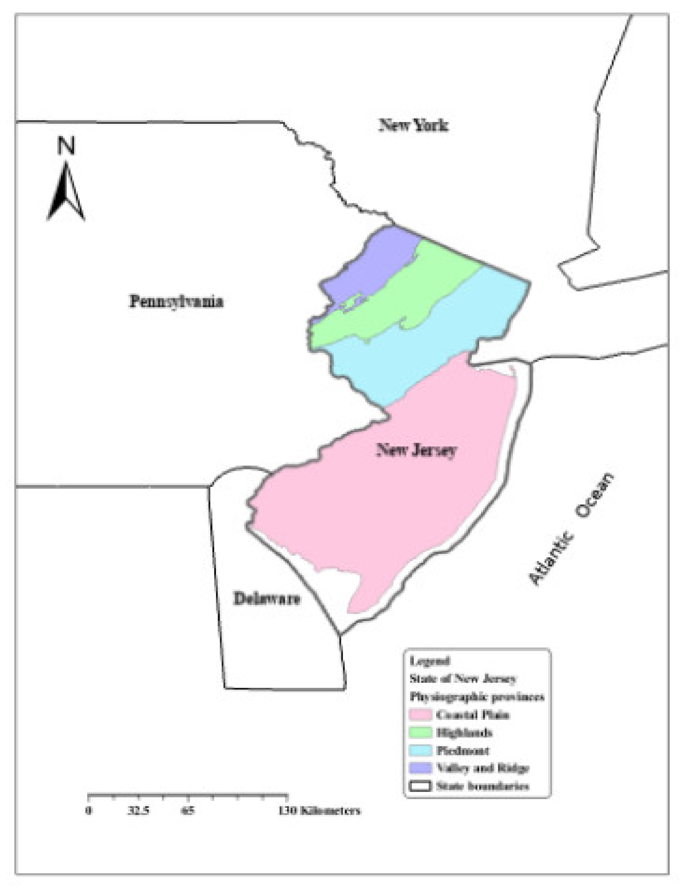
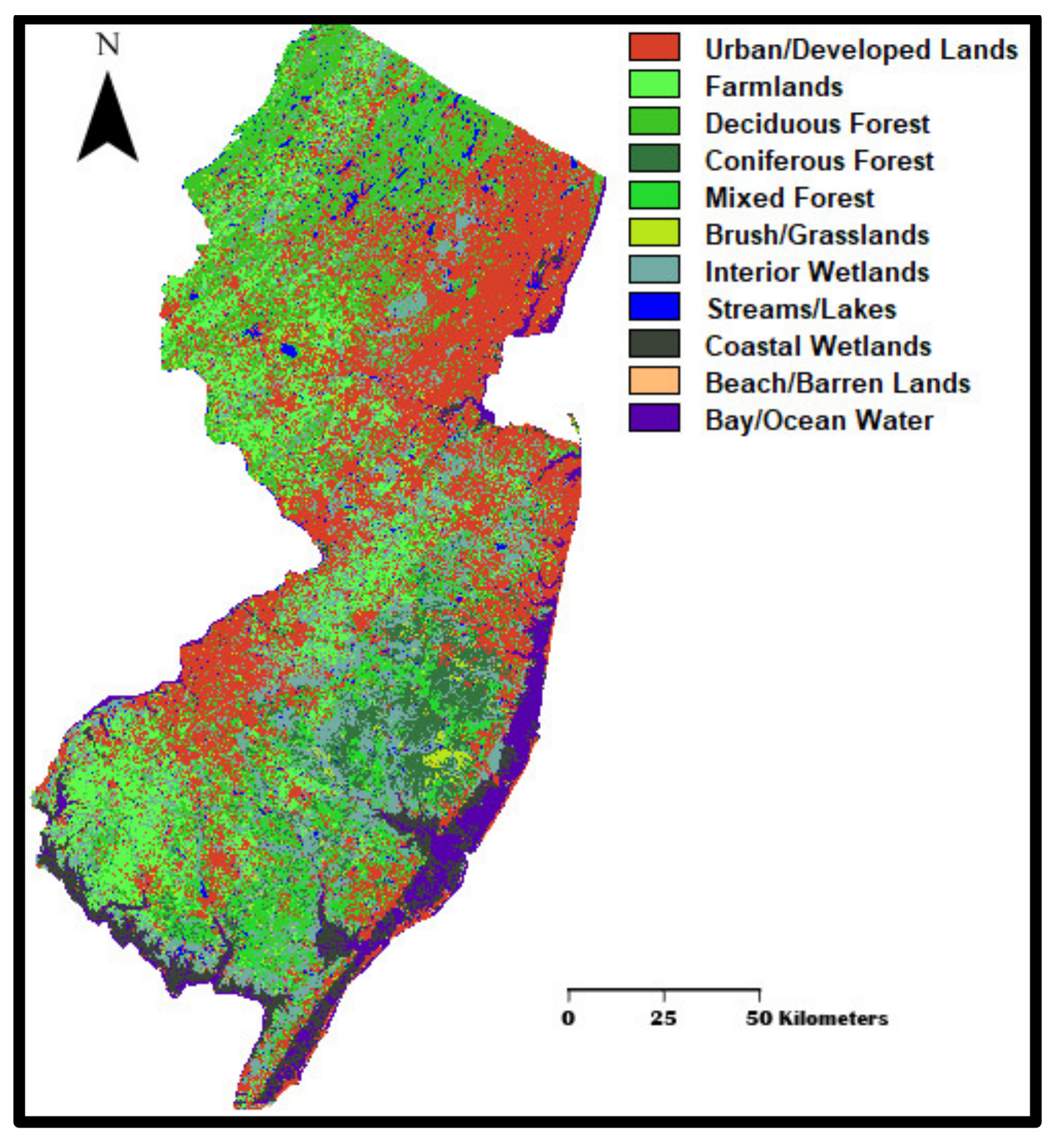
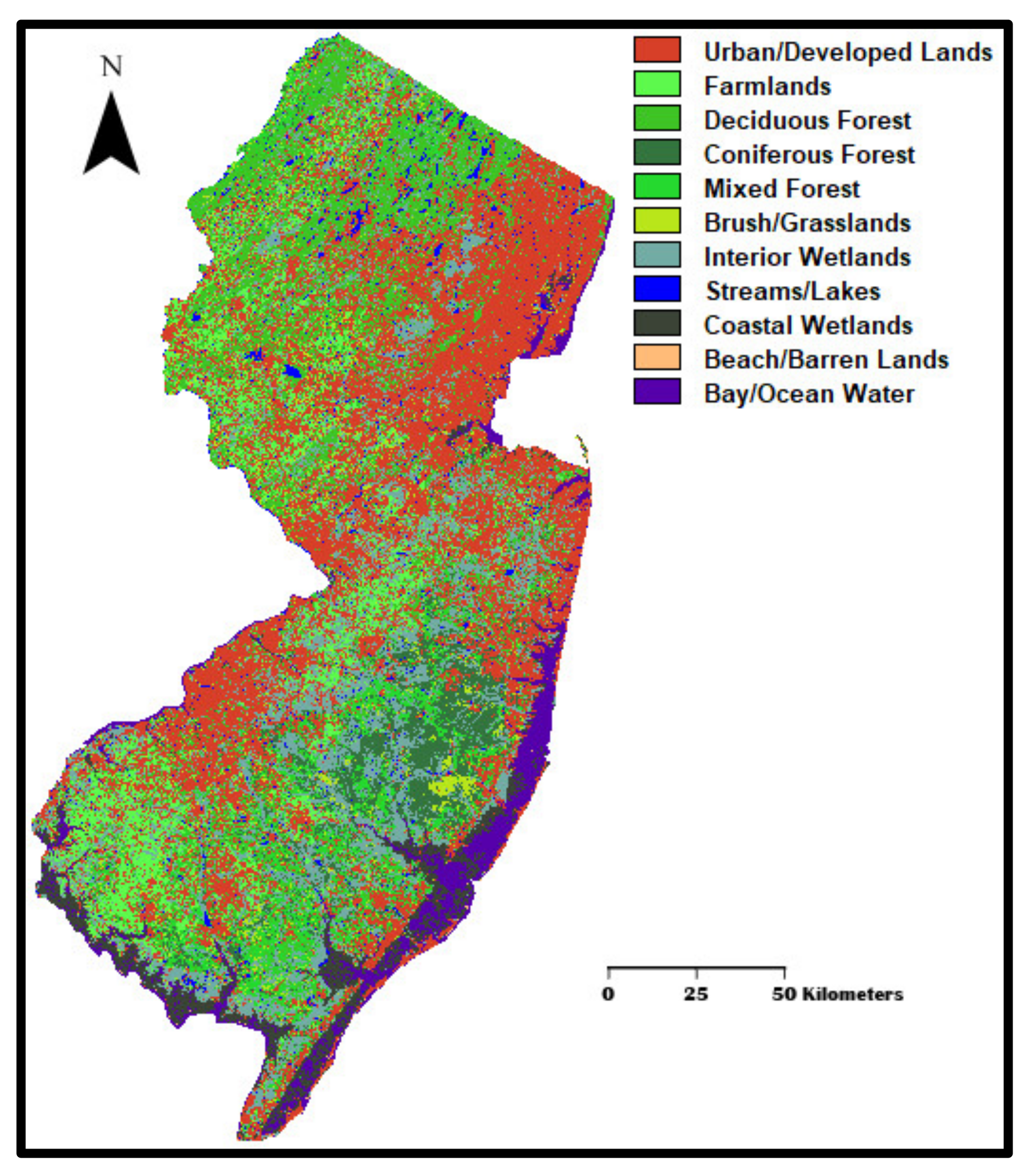
2.1. Study Area
2.2. Data
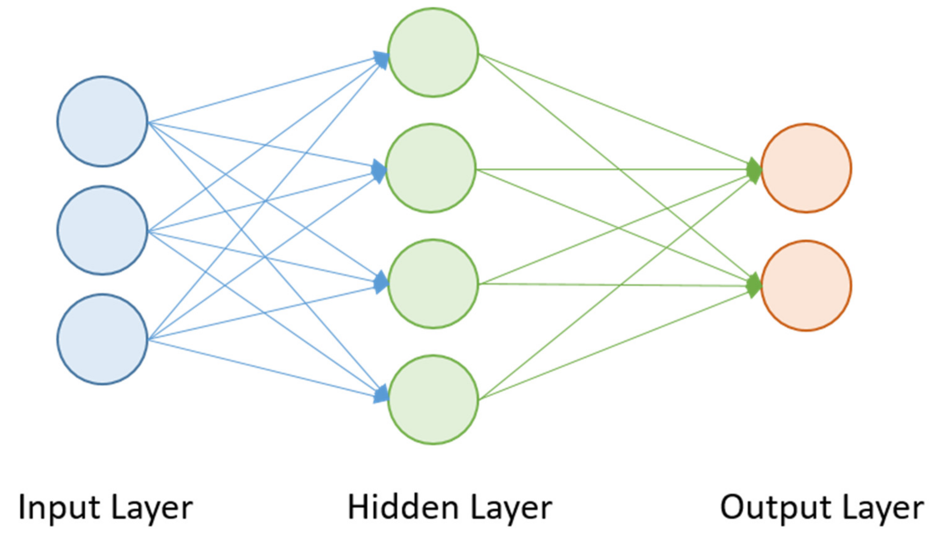
2.3. Method
- (1)
- Change Analysis
- (2)
- Transition potential modeling
- (3)
- Change prediction
- (4)
- Model validation
- (5)
- Land cover analysis
3. Results
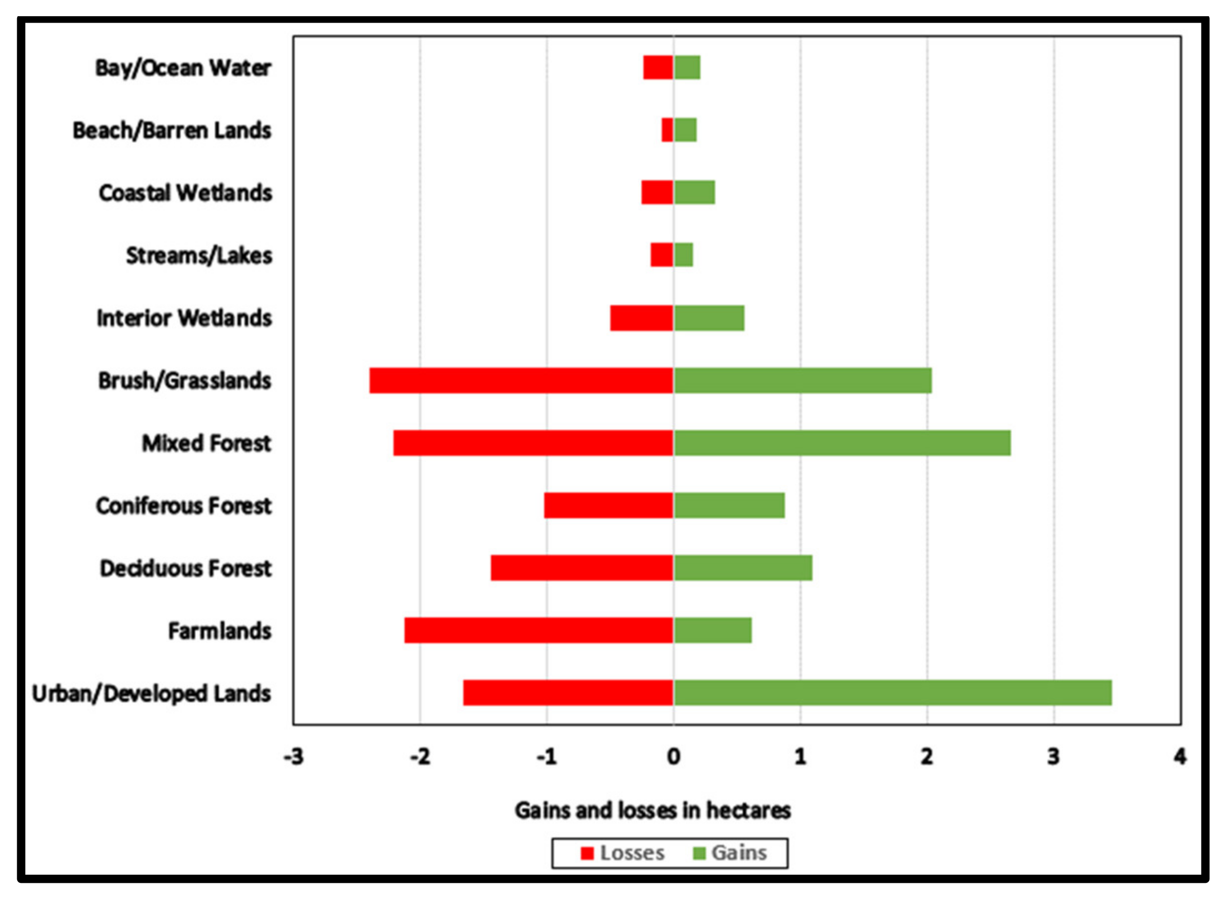
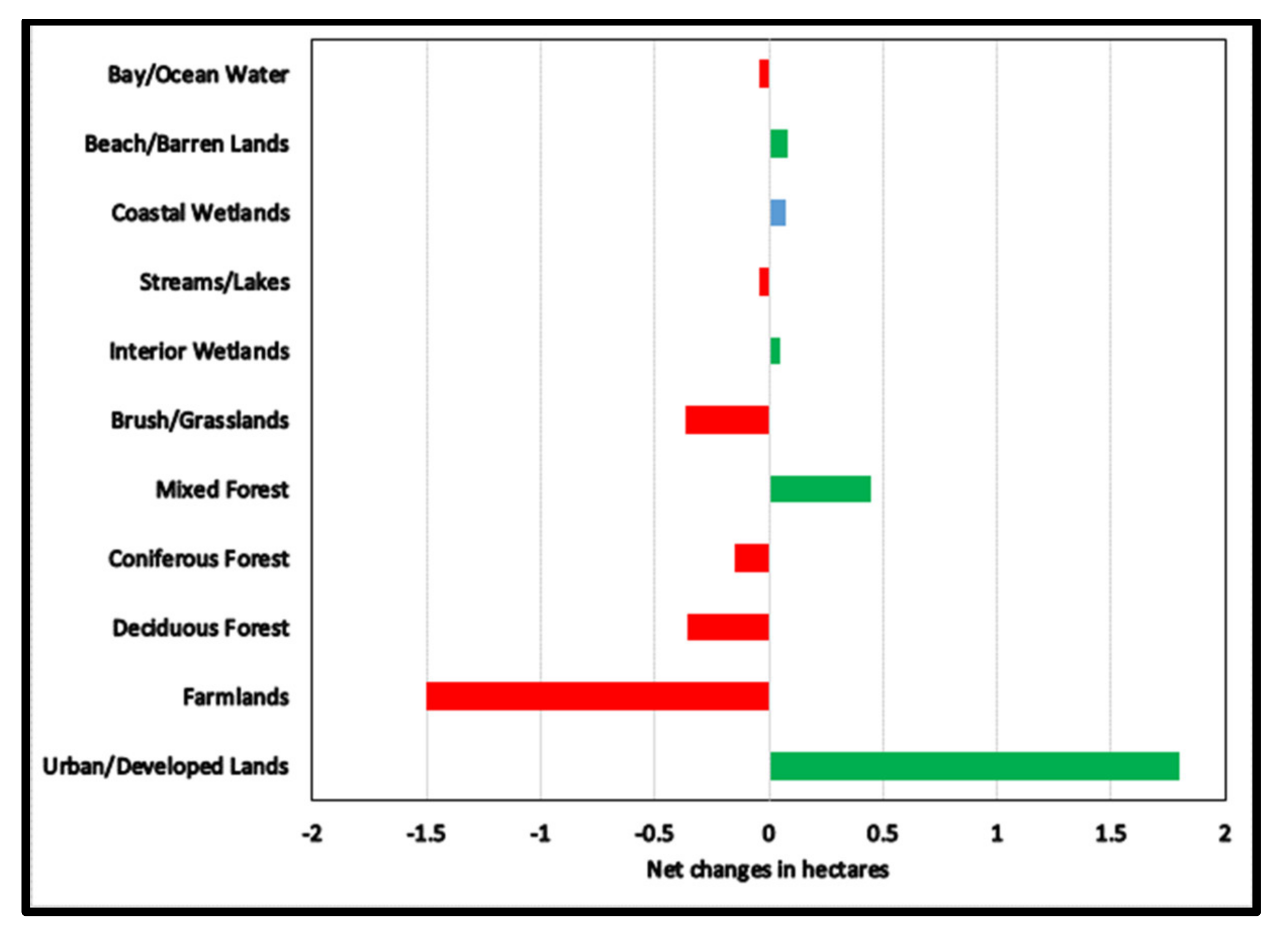
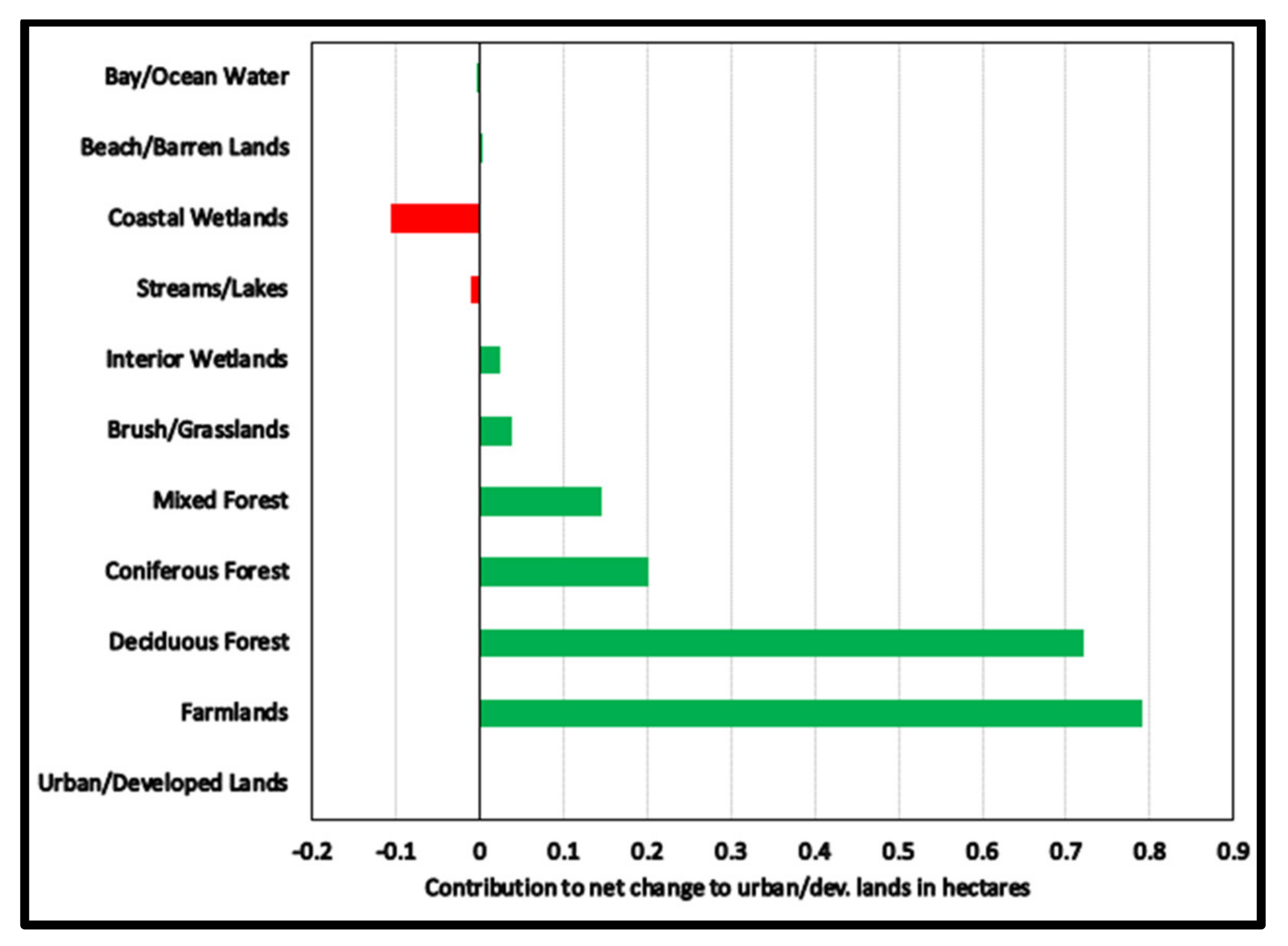
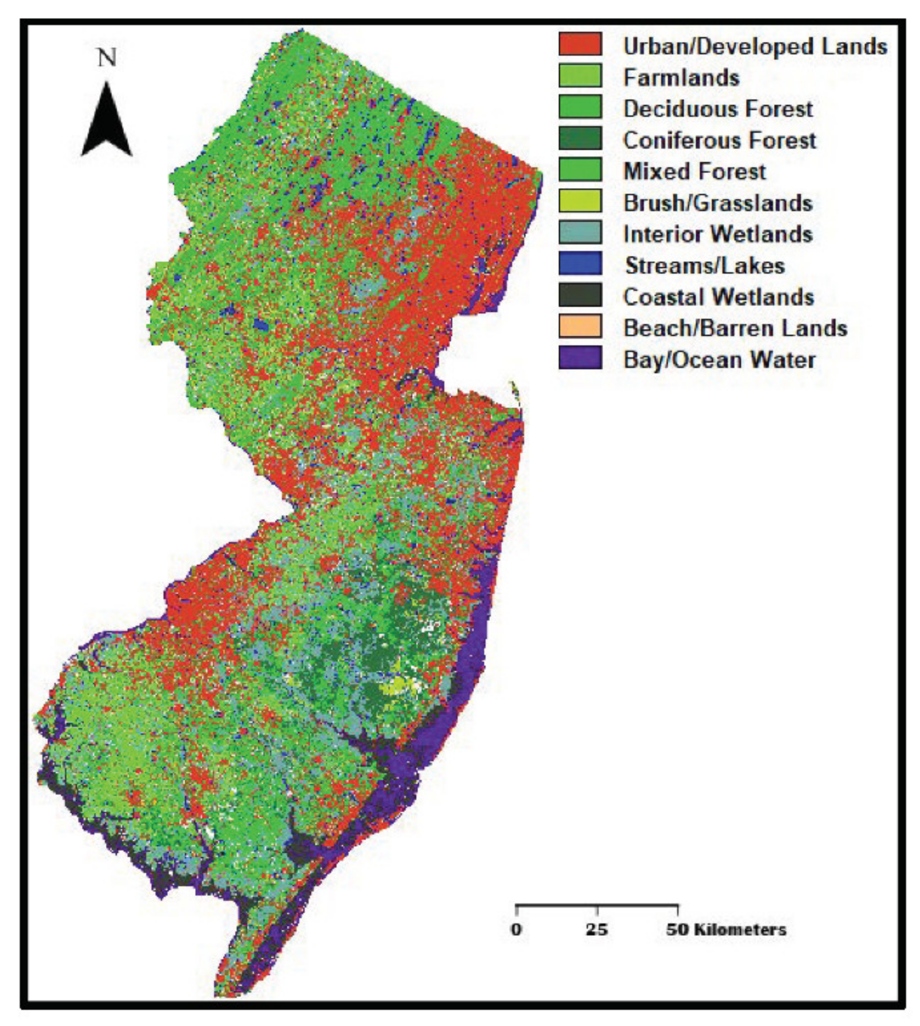
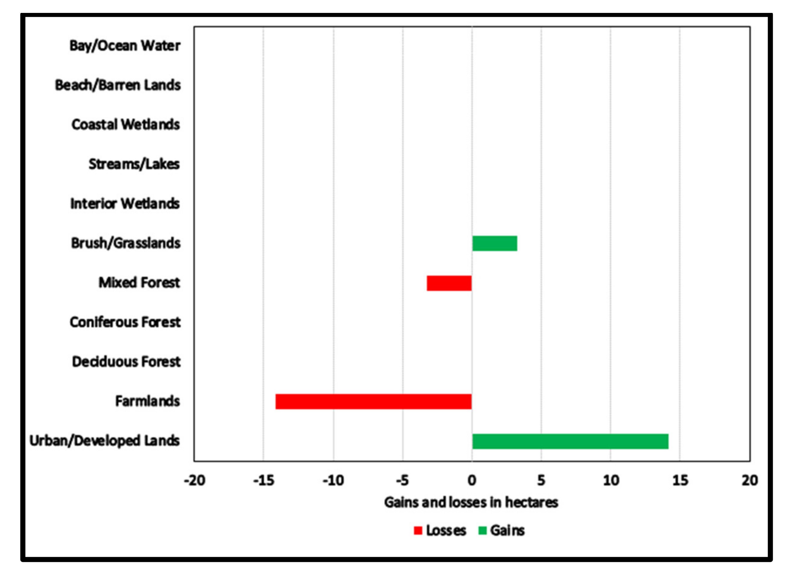
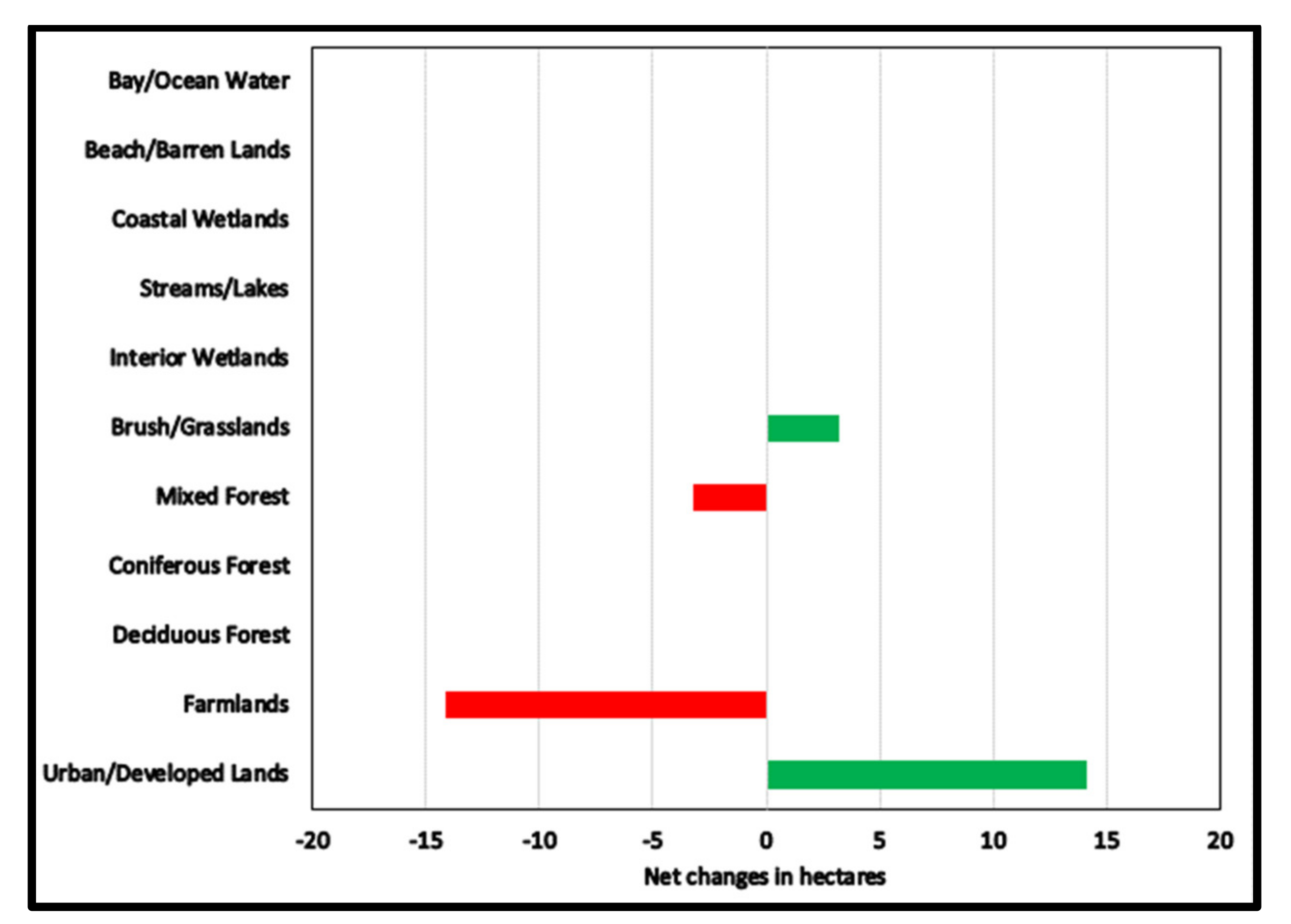
3.1. Land Cover Change between 2007 and 2012
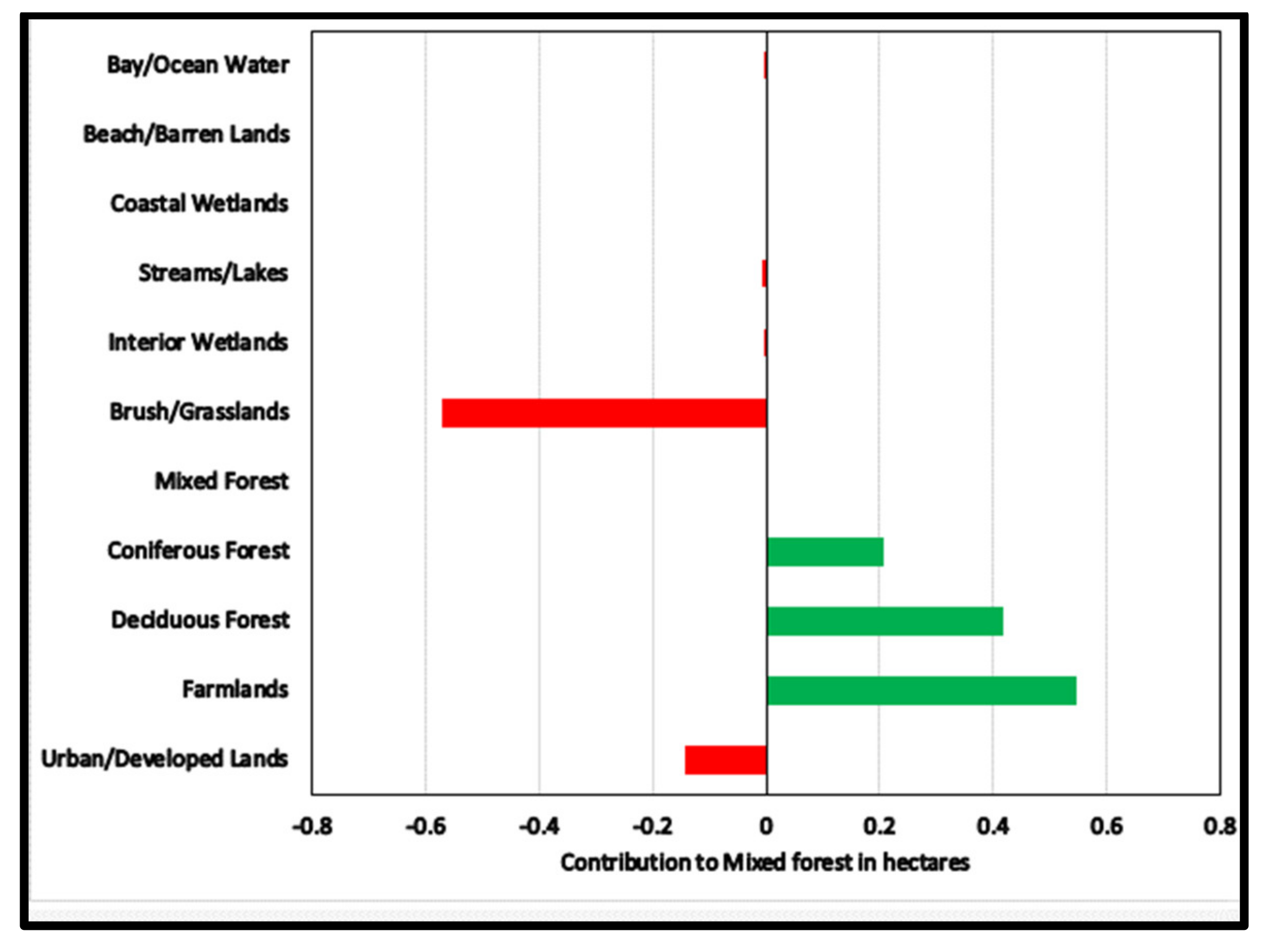
3.2. Transition Model
3.3. Predictions of Land Use Change in 2015 and Model Validation
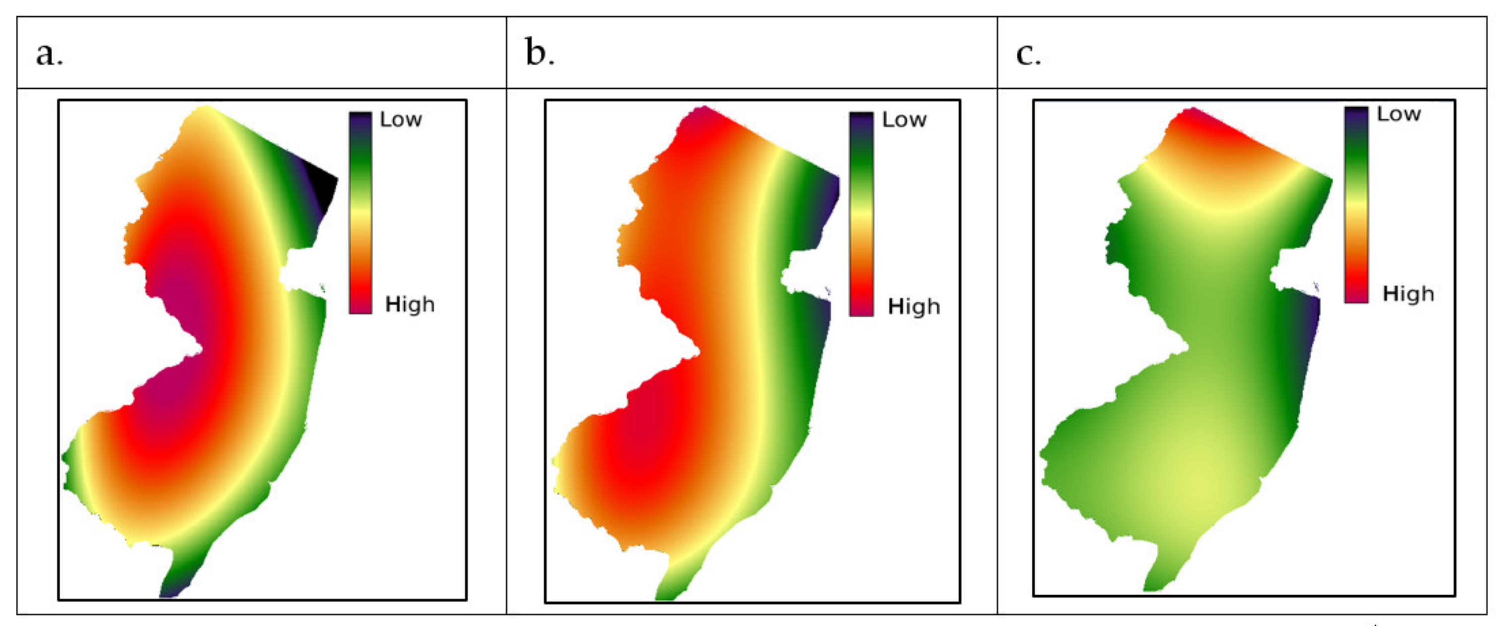
3.4. Prediction of Land Use Change in 2100
4. Discussion and Conclusions
Author Contributions
Funding
Data Availability Statement
Acknowledgments
Conflicts of Interest
Appendix A

| Original LULC Classes | Reclassified LULC Classes |
|---|---|
| Residential, High Density or Multiple Dwelling | Urban/Developed Lands |
| Residential, Single Unit, Medium Density | Urban/Developed Lands |
| Residential, Single Unit, Low Density | Urban/Developed Lands |
| Residential, Rural, Single Unit | Urban/Developed Lands |
| Mixed Residential | Urban/Developed Lands |
| Commercial/Services | Urban/Developed Lands |
| Military Installations | Urban/Developed Lands |
| No Longer Military | Urban/Developed Lands |
| Industrial | Urban/Developed Lands |
| Transportation/Communication/Utilities | Urban/Developed Lands |
| Major Roadway | Urban/Developed Lands |
| Mixed Transportation Corridor Overlap Area | Urban/Developed Lands |
| Bridge Over Water | Urban/Developed Lands |
| Railroads | Urban/Developed Lands |
| Airport Facilities | Urban/Developed Lands |
| Wetland Rights-of-Way | Interior Wetlands |
| Upland Rights-of-Way Developed | Urban/Developed Lands |
| Upland Rights-of-Way Undeveloped | Urban/Developed Lands |
| Stormwater Basin | Urban/Developed Lands |
| Industrial and Commercial Complexes | Urban/Developed Lands |
| Mixed Urban or Built-Up Land | Urban/Developed Lands |
| Other Urban or Built-Up Land | Urban/Developed Lands |
| Cemetery | Urban/Developed Lands |
| Cemetery on Wetland | Urban/Developed Lands |
| Phragmites Dominate Urban Area | Urban/Developed Lands |
| Managed Wetland in Maintained Lawn Greenspace | Urban/Developed Lands |
| Recreational Land | Urban/Developed Lands |
| Athletic Fields (Schools) | Urban/Developed Lands |
| Stadium, Theaters, Cultural Centers and Zoos | Urban/Developed Lands |
| Managed Wetland in Built-Up Maintained Rec Area | Interior Wetlands |
| Cropland and Pastureland | Farmlands |
| Agricultural Wetlands (Modified) | Farmlands |
| Former Agricultural Wetland (Becoming Shrubby, Not Built-Up) | Interior Wetlands |
| Orchards/Vineyards/Nurseries/Horticultural Areas | Farmlands |
| Confined Feeding Operations | Farmlands |
| Other Agriculture | Farmlands |
| Deciduous Forest (10–50% Crown Closure) | Deciduous Forest |
| Deciduous Forest (>50% Crown Closure) | Deciduous Forest |
| Coniferous Forest (10–50% Crown Closure) | Coniferous Forest |
| Coniferous Forest (>50% Crown Closure) | Coniferous Forest |
| Plantation | Farmlands |
| Mixed Forest (>50% Coniferous with 10–50% Crown Closure) | Mixed Forest |
| Mixed Forest (>50% Coniferous with >50% Crown Closure) | Mixed Forest |
| Mixed Forest (>50% Deciduous with 10–50% Crown Closure) | Mixed Forest |
| Mixed Forest (>50% Deciduous with >50% Crown Closure) | Mixed Forest |
| Old Field (<25% Brush Covered) | Mixed Forest |
| Phragmites Dominate Old Field | Brush/Grasslands |
| Deciduous Brush/Shrubland | Brush/Grasslands |
| Coniferous Brush/Shrubland | Brush/Grasslands |
| Mixed Deciduous/Coniferous Brush/Shrubland | Brush/Grasslands |
| Severe Burned Upland Vegetation | Brush/Grasslands |
| Streams and Canals | Streams/Lakes |
| Exposed Flats | Streams/Lakes |
| Natural Lakes | Streams/Lakes |
| Artificial Lakes | Streams/Lakes |
| Tidal Rivers, Inland Bays and Other Tidal Waters | Bay/Ocean Water |
| Open Tidal Bays | Bay/Ocean Water |
| Tidal Mud Flat | Bay/Ocean Water |
| Dredged Lagoon | Bay/Ocean Water |
| Atlantic Ocean | Bay/Ocean Water |
| Saline Marsh (Low Marsh) | Coastal Wetlands |
| Saline Marsh (High Marsh) | Coastal Wetlands |
| Freshwater Tidal Marshes | Coastal Wetlands |
| Vegetated Dune Communities | Brush/Grasslands |
| Phragmites Dominate Coastal Wetlands | Coastal Wetlands |
| Deciduous Wooded Wetlands | Interior Wetlands |
| Coniferous Wooded Wetlands | Interior Wetlands |
| Atlantic White Cedar Wetlands | Interior Wetlands |
| Deciduous Scrub/Shrub Wetlands | Interior Wetlands |
| Coniferous Scrub/Shrub Wetlands | Interior Wetlands |
| Mixed Scrub/Shrub Wetlands (Deciduous Dom.) | Interior Wetlands |
| Mixed Scrub/Shrub Wetlands (Coniferous Dom.) | Interior Wetlands |
| Herbaceous Wetlands | Interior Wetlands |
| Phragmites Dominate Interior Wetlands | Interior Wetlands |
| Mixed Wooded Wetlands (Deciduous Dom.) | Interior Wetlands |
| Mixed Wooded Wetlands (Coniferous Dom.) | Interior Wetlands |
| Unvegetated Flats | Interior Wetlands |
| Severe Burned Wetland Vegetation | Interior Wetlands |
| Beaches | Beach/Barren Lands |
| Bare Exposed Rock, Rock Slides, Etc. | Beach/Barren Lands |
| Extractive Mining | Urban/Developed Lands |
| Altered Lands | Urban/Developed Lands |
| Disturbed Wetlands (Modified) | Interior Wetlands |
| Disturbed Tidal Wetlands | Coastal Wetlands |
| Transitional Areas | Beach/Barren Lands |
| Undifferentiated Barren Lands | Beach/Barren Lands |
References
- Fisher, P.; Comber, A.; Wadsworth, R. Land Use and Land Cover: Contradiction or Complement. In Re-Presenting GIS; Fisher, P., Unwin, D.J., Eds.; John Wiley and Sons Ltd.: Leicester, UK, 2005. [Google Scholar]
- Di Gregorio, A.; Jansen, L.J.M. Land Cover Classification System—Classification Concepts and User Manual; Environment and Natural Resources Series; Food and Agriculture Organization of the United Nations: Rome, Italy, 2005. [Google Scholar]
- National Oceanic and Atmospheric Administration (NOAA). What Is the Difference between Land Cover and Land Use? Available online: https://oceanservice.noaa.gov/facts/lclu.html (accessed on 13 August 2021).
- Latham, J.S.; He, C.; Alinovi, L.; DiGregorio, A.; Kalensky, Z. FAO Methodologies for Land Cover Classification and Mapping. In Linking People, Place, and Policy: A GIScience Approach; Walsh, S.J., Crews-Meyer, K.A., Eds.; Springer: Boston, MA, USA, 2002; pp. 283–316. [Google Scholar] [CrossRef]
- Meyer, W.B.; Turner, B.L. Human Population Growth and Global Land-Use/Cover Change. Annu. Rev. Ecol. Syst. 1992, 2, 39–61. [Google Scholar] [CrossRef]
- Uvsh, D.; Gehlbach, S.; Potapov, P.V.; Munteanu, C.; Bragina, E.V.; Radeloff, V.C. Correlates of Forest-Cover Change in European Russia, 1989–2012. Land Use Policy 2020, 96, 104648. [Google Scholar] [CrossRef]
- Bracchetti, L.; Carotenuto, L.; Catorci, A. Land-Cover Changes in a Remote Area of Central Apennines (Italy) and Management Directions. Landsc. Urban Plan. 2012, 104, 157–170. [Google Scholar] [CrossRef]
- Crews-Meyer, K.A. Agricultural Landscape Change and Stability in Northeast Thailand: Historical Patch-Level Analysis. Agric. Ecosyst. Environ. 2004, 101, 155–169. [Google Scholar] [CrossRef]
- Zheng, Z.; Wu, Z.; Chen, Y.; Yang, Z.; Marinello, F. Exploration of Eco-Environment and Urbanization Changes in Coastal Zones: A Case Study in China over the Past 20 Years. Ecol. Indic. 2020, 119, 106847. [Google Scholar] [CrossRef]
- Jasinski, E.; Morton, D.; DeFries, R.; Shimabukuro, Y.; Anderson, L.; Hansen, M. Physical Landscape Correlates of the Expansion of Mechanized Agriculture in Mato Grosso, Brazil. Earth Interact. 2005, 9, 1–18. [Google Scholar] [CrossRef] [Green Version]
- Hailu, A.; Mammo, S.; Kidane, M. Dynamics of Land Use, Land Cover Change Trend and Its Drivers in Jimma Geneti District, Western Ethiopia. Land Use Policy 2020, 99, 105011. [Google Scholar] [CrossRef]
- Abd El-Kawy, O.R.; El-Kawy, O.R.A.; Rød, J.K.; Ismail, H.A.; Suliman, A.S. Land Use and Land Cover Change Detection in the Western Nile Delta of Egypt Using Remote Sensing Data. Appl. Geogr. 2011, 31, 483–494. [Google Scholar] [CrossRef]
- Vågen, T.-G. Remote Sensing of Complex Land Use Change Trajectories—A Case Study from the Highlands of Madagascar. Agric. Ecosyst. Environ. 2006, 115, 219–228. [Google Scholar] [CrossRef]
- Kindu, M.; Schneider, T.; Teketay, D.; Knoke, T. Land Use/Land Cover Change Analysis Using Object-Based Classification Approach in Munessa-Shashemene Landscape of the Ethiopian Highlands. Remote Sens. 2013, 5, 2411. [Google Scholar] [CrossRef] [Green Version]
- Demissie, F.; Yeshitila, K.; Kindu, M.; Schneider, T. Land Use/Land Cover Changes and Their Causes in Libokemkem District of South Gonder, Ethiopia. Remote Sens. Appl. Soc. Environ. 2017, 8, 224–230. [Google Scholar] [CrossRef]
- Asenso Barnieh, B.; Jia, L.; Menenti, M.; Zhou, J.; Zeng, Y. Mapping Land Use Land Cover Transitions at Different Spatiotemporal Scales in West Africa. Sustainability 2020, 12, 8565. [Google Scholar] [CrossRef]
- Chimi, C.; Tenzin, J.; Cheki, T. Assessment of Land Use/Cover Change and Urban Expansion Using Remote Sensing and GIS: A Case Study in Phuentsholing Municipality, Chukha, Bhutan. Int. J. Energy Environ. Sci. 2017, 2, 127–135. [Google Scholar] [CrossRef]
- Elmahdy, S.; Mohamed, M.; Ali, T. Land Use/Land Cover Changes Impact on Groundwater Level and Quality in the Northern Part of the United Arab Emirates. Remote Sens. 2020, 12, 1715. [Google Scholar] [CrossRef]
- Montalván-Burbano, N.; Velastegui-Montoya, A.; Gurumendi-Noriega, M.; Morante-Carballo, F.; Adami, M. Worldwide Research on Land Use and Land Cover in the Amazon Region. Sustainability 2021, 13, 6039. [Google Scholar] [CrossRef]
- Talukdar, S.; Singha, P.; Mahato, S.; Shahfahad; Pal, S.; Liou, Y.-A.; Rahman, A. Land-Use Land-Cover Classification by Machine Learning Classifiers for Satellite Observations—A Review. Remote Sens. 2020, 12, 1135. [Google Scholar] [CrossRef] [Green Version]
- Maxwell, A.E.; Warner, T.A.; Fang, F. Implementation of Machine-Learning Classification in Remote Sensing: An Applied Review. Int. J. Remote. Sens. 2018, 39, 2784–2817. [Google Scholar] [CrossRef] [Green Version]
- Mubea, K.W.; Ngigi, T.G.; Mundia, C.N. Assessing Application of Markov Chain Analysis in Predicting Land Cover Change: A Case Study of Nakuru Municipality. J. Agric. Sci. Technol. 2011, 12, 182–188. [Google Scholar]
- Islam, M.S.; Ahmed, R. Land Use Change Prediction in Dhaka City Using Gis Aided Markov Chain Modeling. J. Life Earth Sci. 2011, 6, 81–89. [Google Scholar] [CrossRef] [Green Version]
- Iacono, M.; Levinson, D.; El-Geneidy, A.; Wasfi, R. A Markov Chain Model of Land Use Change. TeMA—J. Land Use Mobil. Environ. 2015, 8, 263–276. [Google Scholar] [CrossRef]
- Hua, A.K. Application Of CA-Markov Model and Land Use/Land Cover Changes in Malacca River Watershed, Malaysia. Appl. Ecol. Environ. Res. 2017, 15, 605–622. [Google Scholar] [CrossRef]
- Rimal, B.; Zhang, L.; Keshtkar, H.; Wang, N.; Lin, Y. Monitoring and Modeling of Spatiotemporal Urban Expansion and Land-Use/Land-Cover Change Using Integrated Markov Chain Cellular Automata Model. ISPRS Int. J. Geo-Inf. 2017, 6, 288. [Google Scholar] [CrossRef] [Green Version]
- Surabuddin Mondal, M.; Sharma, N.; Kappas, M.; Garg, P.K. CA Markov Modeling of Land Use Land Cover Dynamics And Sensitivity Analysis To Identify Sensitive Parameter(S). Int. Arch. Photogramm. Remote Sens. Spatial Inf. Sci. 2019, XLII-2/W13, 723–729. [Google Scholar] [CrossRef] [Green Version]
- Lai, Y.; Huang, G.; Chen, S.; Lin, S.; Lin, W.; Lyu, J. Land Use Dynamics and Optimization from 2000 to 2020 in East Guangdong Province, China. Sustainability 2021, 13, 3473. [Google Scholar] [CrossRef]
- Eastman, J.R.; He, J. A Regression-Based Procedure for Markov Transition Probability Estimation in Land Change Modeling. Land 2020, 9, 407. [Google Scholar] [CrossRef]
- Guo, A.; Zhang, Y.; Hao, Q. Monitoring and Simulation of Dynamic Spatiotemporal Land Use/Cover Changes. Complexity 2020, 2020, e3547323. [Google Scholar] [CrossRef]
- Shen, L.; Li, J.; Wheate, R.; Yin, J.; Paul, S. Multi-Layer Perceptron Neural Network and Markov Chain Based Geospatial Analysis of Land Use and Land Cover Change. J. Environ. Inform. Lett. 2020, 3, 29–39. [Google Scholar] [CrossRef]
- Dadhich, P.N.; Hanaoka, S. Markov Method Integration with Multi-Layer Perceptron Classifier for Simulation of Urban Growth of Jaipur City. In Proceedings of the 6th International Conference on Remote Sensing, Iwate, Japan, 4–6 October 2010; pp. 118–123. [Google Scholar]
- Iizuka, K.; Johnson, B.A.; Onishi, A.; Magcale-Macandog, D.B.; Endo, I.; Bragais, M. Modeling Future Urban Sprawl and Landscape Change in the Laguna de Bay Area, Philippines. Land 2017, 6, 26. [Google Scholar] [CrossRef]
- Pereira e Silva, L.; Xavier, A.P.C.; da Silva, R.M.; Santos, C.A.G. Modeling Land Cover Change Based on an Artificial Neural Network for a Semiarid River Basin in Northeastern Brazil. Glob. Ecol. Conserv. 2020, 21, e00811. [Google Scholar] [CrossRef]
- Ozturk, D. Urban Growth Simulation of Atakum (Samsun, Turkey) Using Cellular Automata-Markov Chain and Multi-Layer Perceptron-Markov Chain Models. Remote Sens. 2015, 7, 5918–5950. [Google Scholar] [CrossRef] [Green Version]
- The Geography of New Jersey. Available online: https://www.netstate.com/states/geography/nj_geography.htm (accessed on 28 July 2021).
- Wacker, P.O. New Jersey State, United States. Available online: https://www.britannica.com/place/New-Jersey (accessed on 28 July 2021).
- Salisbury, R.D. The Physical Geography of New Jersey; Geological Survey of New Jersey: Trenton, NJ, USA, 1808; p. 400. [Google Scholar]
- New Jersey—New World Encyclopedia. Available online: https://www.newworldencyclopedia.org/entry/New_Jersey (accessed on 28 July 2021).
- Zimmer, D.M. What New Jersey 2020 Census Results Reveal About State’s Population. Available online: https://www.northjersey.com/story/news/new-jersey/2021/08/12/nj-population-2021-by-county-growth-2020-census-results/8113856002/ (accessed on 19 September 2021).
- Population Density in the U.S., by State 2020. Available online: https://www.statista.com/statistics/183588/population-density-in-the-federal-states-of-the-us/ (accessed on 30 July 2021).
- List of U.S. States by Population Density. 2021. Available online: https://simple.wikipedia.org/wiki/List_of_U.S._states_by_population_density (accessed on 30 July 2021).
- US Census Bureau. State Population Totals: 2010–2020. Available online: https://www.census.gov/programs-surveys/popest/technical-documentation/research/evaluation-estimates/2020-evaluation-estimates/2010s-state-total.html (accessed on 27 July 2021).
- World Population Review. Population of Counties in New Jersey. 2021. Available online: https://worldpopulationreview.com/us-counties/states/nj (accessed on 31 July 2021).
- New Jersey Department of Labor and Workforce Development. 2020 Population Density: New Jersey Counties. 2021. Available online: https://www.nj.gov/labor/lpa/content/maps/Popden.pdf (accessed on 1 August 2021).
- New Jersey Department of Environmental Protection. 2012 Land Use/Land Cover Update and Impervious Surface Mapping Project. Available online: https://www.nj.gov/dep/gis/digidownload/metadata/lulc12/update2012.html (accessed on 25 August 2021).
- Esri. 2D, 3D & 4D GIS Mapping Software|ArcGIS Pro. Available online: https://www.esri.com/en-us/arcgis/products/arcgis-pro/overview (accessed on 14 October 2021).
- Clark University. TerrSet 2020 Software Features. Available online: https://clarklabs.org/ (accessed on 7 August 2021).
- Orrù, P.F.; Zoccheddu, A.; Sassu, L.; Mattia, C.; Cozza, R.; Arena, S. Machine Learning Approach Using MLP and SVM Algorithms for the Fault Prediction of a Centrifugal Pump in the Oil and Gas Industry. Sustainability 2020, 12, 4776. [Google Scholar] [CrossRef]
- Hastie, T.; Tibshirani, R.; Friedman, J. The Elements of Statistical Learning: Data Mining, Inference, and Prediction, 2nd ed.; Springer Series in Statistics; Springer: New Yok, NY, USA, 2017; Available online: https://web.stanford.edu/~hastie/ElemStatLearn/printings/ESLII_print12_toc.pdf (accessed on 17 August 2021).
- Kityuttachai, K.; Tripathi, N.K.; Tipdecho, T.; Shrestha, R. CA-Markov Analysis of Constrained Coastal Urban Growth Modeling: Hua Hin Seaside City, Thailand. Sustainability 2013, 5, 1480–1500. [Google Scholar] [CrossRef] [Green Version]
- Subedi, P.; Subedi, K.; Thapa, B. Application of a Hybrid Cellular Automaton—Markov (CA-Markov) Model in Land-Use Change Prediction: A Case Study of Saddle Creek Drainage Basin, Florida. Appl. Ecol. Environ. Sci. 2013, 1, 126–132. [Google Scholar] [CrossRef] [Green Version]
- Pontius, R.G. Quantification Error Versus Location Error in Comparison of Categorical Maps. Photogramm. Remote Sens. 2000, 66, 1011–1016. [Google Scholar]
- Pontius, R.G. Statistical Methods to Partition Effects of Quantity and Location During Comparison of Categorical Maps at Multiple Resolutions. Photogramm. Eng. Remote 2002, 68, 1041–1049. [Google Scholar]
- Pontius Jr, R.G.; Batchu, K. Using the Relative Operating Characteristic to Quantify Certainty in Prediction of Location of Land Cover Change in India. Trans. GIS 2003, 7, 467–484. [Google Scholar] [CrossRef]
- Ariza-Lopez, F.J.; Rodriguez-Avi, J.; Alba-Fernandez, M.V. Complete Control of an Observed Confusion Matrix. In Proceedings of the IGARSS 2018—2018 IEEE International Geoscience and Remote Sensing Symposium, Valencia, Spain, 22–27 July 2018; pp. 1222–1225. [Google Scholar] [CrossRef]
- Ukrainski, P.; Classification Accuracy Assessment. Confusion Matrix Method. 50 North|GIS Blog from Ukraine. 2016. Available online: http://www.50northspatial.org/classification-accuracy-assessment-confusion-matrix-method/ (accessed on 9 August 2021).
- Lewis, H.G.; Brown, M. A Generalized Confusion Matrix for Assessing Area Estimates from Remotely Sensed Data. Int. J. Remote Sens. 2001, 22, 3223–3235. [Google Scholar] [CrossRef]
- Visa, S.; Ramsay, B.; Ralescu, A.; Knaap, E. Confusion Matrix-Based Feature Selection. In Proceedings of the 22nd Midwest Artificial Intelligence and Cognitive Science Conference 2011, Cincinnati, OH, USA, 16–17 April 2011; Volume 710, p. 127. [Google Scholar]
- Monmonier, M. Measures of Pattern Complexity for Choropleth Maps. Cartogr. Geogr. Inf. Sci. 1974, 1, 159–169. [Google Scholar] [CrossRef]
- Turner, M.G. Landscape Ecology: The Effect of Pattern on Process. Annu. Rev. Ecol. Syst. 1989, 20, 171–197. [Google Scholar] [CrossRef]
- Elmes, A.; Alemohammad, H.; Avery, R.; Caylor, K.; Eastman, J.R.; Fishgold, L.; Friedl, M.A.; Jain, M.; Kohli, D.; Laso Bayas, J.C.; et al. Accounting for Training Data Error in Machine Learning Applied to Earth Observations. Remote Sens. 2020, 12, 1034. [Google Scholar] [CrossRef] [Green Version]
- Saghir, J.; Santoro, J.; Urbanization in Sub-Saharan Africa: Meeting Challenges by Bridging Stakeholders. Center for Strategic and International Studies. 2018. Available online: https://csis-website-prod.s3.amazonaws.com/s3fs-public/publication/180411_Saghir_UrbanizationAfrica_Web.pdf (accessed on 19 September 2021).
- Zhang, Q.; Justice, C.O.; Desanker, P.V. Impacts of Simulated Shifting Cultivation on Deforestation and the Carbon Stocks of the Forests of Central Africa. Agric. Ecosyst. Environ. 2002, 90, 203–209. [Google Scholar] [CrossRef]
- Sola, P.; Cerutti, P.O.; Zhou, W.; Gautier, D.; Iiyama, M.; Schure, J.; Chenevoy, A.; Yila, J.; Dufe, V.; Nasi, R.; et al. The Environmental, Socioeconomic, and Health Impacts of Woodfuel Value Chains in Sub-Saharan Africa: A Systematic Map. Environ. Evid. 2017, 6, 4. [Google Scholar] [CrossRef] [Green Version]
- Paré, S.; Söderberg, U.; Sandewall, M.; Ouadba, J.M. Land Use Analysis from Spatial and Field Data Capture in Southern Burkina Faso, West Africa. Agric. Ecosyst. Environ. 2008, 127, 277–285. [Google Scholar] [CrossRef]
- Bob, U. Land-related conflicts in Sub-Saharan Africa. Available online: https://www.accord.org.za/ajcr-issues/land-related-conflicts-in-sub-saharan-africa/ (accessed on 19 September 2021).
- Peters, P.E. Inequality and Social Conflict Over Land in Africa. J. Agrar. Chang. 2004, 4, 269–314. [Google Scholar] [CrossRef]
- NJDEP-Division of Land Resource Protection-Home. Available online: https://www.nj.gov/dep/landuse/ (accessed on 19 August 2021).
- NJDEP|Land Use Management. Available online: https://www.nj.gov/dep/lum/ (accessed on 19 August 2021).
- NJDEP-Division of Land Use Regulation-Home. Available online: https://www.nj.gov/dep/landuse/process.html (accessed on 19 August 2021).
- Callinan, S. Gentrification of Two New Jersey Cities. Available online: https://storymaps.arcgis.com/stories/e38e09f5c5a045abae1571e9b7cb769d (accessed on 19 August 2021).
- Thompson, J.R.; Carpenter, D.N.; Cogbill, C.V.; Foster, D.R. Four Centuries of Change in Northeastern United States Forests. PLoS ONE 2013, 8, e72540. [Google Scholar] [CrossRef] [PubMed] [Green Version]
- Edwards, J.W.; Dachelet, C.A.; Smathers, W.M. A Mobile Aviary to Enhance Translocation Success of Red-Cockaded Woodpeckers. In Proceedings of the 37th Annual Meeting of the Canadian Society of Environmental Biologists; 1997. Available online: https://www.fs.usda.gov/treesearch/pubs/1959 (accessed on 5 October 2021).
- Flammia, D. NJ Tops Nation for Addressing the Loss of Farmland. Available online: https://nj1015.com/nj-tops-nation-for-addressing-the-loss-of-farmland/ (accessed on 15 October 2021).
- Benincà, E.; Ballantine, B.; Ellner, S.; Huisman, J. Species Fluctuations Sustained by a Cyclic Succession at the Edge of Chaos. Proc. Natl. Acad. Sci. USA 2015, 112, 6389–6394. [Google Scholar] [CrossRef] [Green Version]
- NJDEP New Jersey Department of Environmental Protection. Forest Health in New Jersey. Available online: https://www.state.nj.us/dep/parksandforests/forest/njfs_forest_health.html (accessed on 15 October 2021).
- Fallon, S. New Jersey Prepares for Possible Invasion of Tree-Destroying Bug, the Spotted Lanternfly. Available online: https://www.northjersey.com/story/news/environment/2017/10/08/tree-destroying-bug-on-njs-doorstep/618329001/ (accessed on 27 August 2021).
- Kent, S.; NJ Advance Media for NJ.com. The 12 Grossest Living Things That are Killing N.J.’s Trees. Available online: https://www.nj.com/news/2017/05/greatest_threats_to_njs_trees.html (accessed on 15 October 2021).
- Hayhoe, K.; Wake, C.; Anderson, B.; Liang, X.-Z.; Maurer, E.; Zhu, J.; Bradbury, J.; DeGaetano, A.; Stoner, A.M.; Wuebbles, D. Regional Climate Change Projections for the Northeast USA. Mitig. Adapt. Strateg. Glob. Chang. 2008, 13, 425–436. [Google Scholar] [CrossRef]
- The New Jersey Climate Change Resource Center. Climate Change in New Jersey: Impacts and Responses, Rutgers, The State University of New Jersey. 2020. Available online: https://njclimateresourcecenter.rutgers.edu/ (accessed on 5 October 2021).
- Janowiak, M.K.; D’Amato, A.W.; Swanston, C.W.; Iverson, L.; Thompson, F.R.; Dijak, W.D.; Matthews, S.; Peters, M.P.; Prasad, A.; Fraser, J.S.; et al. New England and Northern New York Forest Ecosystem Vulnerability Assessment and Synthesis: A Report from the New England Climate Change Response Framework Project; NRS-GTR-173; U.S. Department of Agriculture, Forest Service, Northern Research Station: Newtown Square, PA, USA, 2018. [Google Scholar] [CrossRef]
- Evans, A.; Mahaffey, A. Restoration and Resilience in New Jersey’s Forests; ForesGUILD: Santa Fe, NM, USA, 2014; Available online: https://foreststewardsguild.org/wp-content/uploads/2019/05/New_Jersey.pdf (accessed on 7 October 2021).
- Ngoy, K.I.; Shebitz, D. Potential Impacts of Climate Change on Areas Suitable to Grow Some Key Crops in New Jersey, USA. Environments 2020, 7, 76. [Google Scholar] [CrossRef]
- Environmental Law Institute. Land Use. Available online: https://www.eli.org/keywords/land-use (accessed on 15 October 2021).
- Cammenga, J. Where Did Americans Move in 2020? 2021. Available online: https://taxfoundation.org/state-migration-trends/ (accessed on 7 October 2021).
- Loomis, E. Forests and Logging in the United States. Available online: https://oxfordre.com/americanhistory/view/10.1093/acrefore/9780199329175.001.0001/acrefore-9780199329175-e-188 (accessed on 15 October 2021). [CrossRef]


| Name of Component | Definition |
|---|---|
| Disagreement due to quantity | P(p) − P(m) |
| Disagreement at stratum level | P(m) − K(m) |
| Disagreement at grid cell level | K(m) − M(m) |
| Agreement at grid cell level | MAX [M(m) − H(m), 0] |
| Agreement at stratum level | MAX [H(m) − N(m), 0] |
| Agreement due to quantity | If MIN [N(n), N(m), H(m), M(m)] = N(n), then MIN [N(m) − N(n), H(m) − N(n), M(m) − N(n)], else 0 |
| Agreement due to chance | MIN [N(n), N(m), H(m), M(m)] |
| Predicted Image | |||||
|---|---|---|---|---|---|
| A | B | C | Total | ||
| Classified image | a | aA | aB | aC | ∑a |
| b | bA | bB | bC | ∑b | |
| c | cA | cB | cC | ∑c | |
| Total | ∑A | ∑B | ∑C | N = grand total | |
| (a) | |||
| Model | Accuracy (%) | Skill Measure | Influence Order |
| With all variables | 83.32 | 0.7776 | N/A |
| Var. 1 constant | 35.25 | 0.1367 | 1 (most influential) |
| Var. 2 constant | 92.4 | 0.8986 | 3 (least influential) |
| Var. 3 constant | 56.24 | 0.4165 | 2 |
| (b) | |||
| Model | Accuracy (%) | Skill Measure | |
| With all variables | 83.32 | 0.7776 | |
| Step 1: var. [2] constant | 92.4 | 0.8986 | |
| Step 2: var. [2,3] constant | 50 | 0.3334 | |
| (c) | |||
| Class | Skill Measure | ||
| Transition: Farmlands to Urban/Developed Lands | 0.9146 | ||
| Transition: Mixed Forest to Brush/Grasslands | 1 | ||
| Persistence: Farmlands | 0.839 | ||
| Persistence: Mixed Forest | 0.3561 |
| Probability of Changing to These Classes | ||||||||||||
|---|---|---|---|---|---|---|---|---|---|---|---|---|
| Urban/ Developed Lands | Farmlands | Deciduous Forest | Coniferous Forest | Mixed Forest | Brush/ Grasslands | Interior Wetlands | Streams/Lakes | Coastal Wetlands | Beach/ Barren Lands | Bay/ Ocean Water | ||
| Given these classes | Urban/ Developed Lands | 0.9942 | 0.0008 | 0.0002 | 0 | 0.0015 | 0.0011 | 0.0014 | 0.0003 | 0.0005 | 0 | 0 |
| Farmlands | 0.0102 | 0.979 | 0 | 0 | 0.0074 | 0.0033 | 0 | 0.0001 | 0 | 0 | 0 | |
| Deciduous Forest | 0.0055 | 0.0004 | 0.9896 | 0 | 0.0041 | 0.0003 | 0.0001 | 0 | 0 | 0 | 0 | |
| Coniferous Forest | 0.0038 | 0.0002 | 0.0002 | 0.9805 | 0.009 | 0.0061 | 0 | 0.0001 | 0 | 0 | 0 | |
| Mixed Forest | 0.0091 | 0.0031 | 0.0021 | 0.0042 | 0.9638 | 0.0174 | 0.0001 | 0.0001 | 0 | 0 | 0 | |
| Brush/ Grasslands | 0.0158 | 0.0049 | 0.0403 | 0.028 | 0.0216 | 0.889 | 0.0001 | 0.0002 | 0.0001 | 0 | 0 | |
| Interior Wetlands | 0.0031 | 0.0001 | 0 | 0 | 0 | 0 | 0.9964 | 0.0003 | 0 | 0 | 0 | |
| Streams/ Lakes | 0.0034 | 0.0001 | 0 | 0 | 0.0002 | 0 | 0.0066 | 0.9894 | 0.0001 | 0 | 0.0001 | |
| Coastal Wetlands | 0.0011 | 0 | 0 | 0 | 0 | 0 | 0.0001 | 0 | 0.9929 | 0.0014 | 0.0044 | |
| Beach/ Barren Lands | 0.0063 | 0 | 0 | 0.0006 | 0.0045 | 0.008 | 0.0002 | 0 | 0.0728 | 0.854 | 0.0537 | |
| Bay/Ocean Water | 0.0001 | 0 | 0 | 0 | 0 | 0 | 0 | 0 | 0.0029 | 0.003 | 0.994 | |
| Information of Quantity | |||
|---|---|---|---|
| Information of Allocation | No(n) | Medium(m) | Perfect(p) |
| Perfect[P(x)] | P(n) = 0.5235 | P(m) = 0.9982 | P(p) = 1.0000 |
| PerfectStratum[K(x)] | K(n) = 0.5235 | K(m) = 0.9982 | K(p) = 1.0000 |
| MediumGrid[M(x)] | M(n) = 0.4909 | M(m) = 0.9506 | M(p) = 0.9492 |
| MediumStratum[H(x)] | H(n) = 0.0833 | H(m) = 0.2720 | H(p) = 0.2722 |
| No[N(x)] | N(n) = 0.0833 | N(m) = 0.2720 | N(p) = 0.2722 |
| AgreementChance | 0.0833 | ||
| AgreementQuantity | 0.1887 | ||
| AgreementStrata | 0.0000 | ||
| AgreementGridcell | 0.6785 | ||
| DisagreeGridcell | 0.0476 | ||
| DisagreeStrata | 0.0000 | ||
| DisagreeQuantity | 0.0018 | ||
| Kno | 0.9461 | ||
| Klocation | 0.9344 | ||
| KlocationStrata | 0.9344 | ||
| Kstandard | 0.9321 | ||
| Predicted Land Cover in 2015 | ||||||||||||||
|---|---|---|---|---|---|---|---|---|---|---|---|---|---|---|
| Category | Urban/ Developed Lands | Farmlands | Deci Duous Forest | Coni Ferous Forest | Mixed Forest | Brush/ Grasslands | Interior Wetlands | Streams Lakes | Coastal Wetlands | Beach/ Barren Lands | Bay/ Ocean Water | Total | User’s Accuracy | |
| Classified Land Cover in 2015 | Urban/ Developed Lands | 1,625,588 | 18,535 | 65,138 | 3359 | 9751 | 11,040 | 25,682 | 6173 | 867 | 124 | 1135 | 1,767,392 | 0.919767 |
| Farmlands | 20,867 | 538,568 | 14,156 | 665 | 3778 | 4074 | 9626 | 875 | 4 | 1 | 5 | 592,619 | 0.908793 | |
| Deciduous Forest | 60,701 | 13,337 | 705,797 | 3699 | 12,423 | 6740 | 28,548 | 4635 | 110 | 125 | 103 | 836,218 | 0.844035 | |
| Coniferous Forest | 1707 | 535 | 2273 | 305,392 | 1868 | 983 | 1165 | 227 | 27 | 15 | 2 | 314,194 | 0.971985 | |
| Mixed Forest | 7352 | 3252 | 11,366 | 3017 | 334,737 | 8947 | 4385 | 807 | 33 | 16 | 53 | 373,965 | 0.895102 | |
| Brush/Grasslands | 9791 | 3756 | 6793 | 1111 | 3465 | 100,880 | 3512 | 547 | 80 | 22 | 115 | 130,072 | 0.77557 | |
| Interior Wetlands | 24,064 | 10,242 | 27,188 | 1190 | 4141 | 3868 | 776,431 | 7171 | 323 | 14 | 186 | 854,818 | 0.9083 | |
| Streams/Lakes | 5484 | 707 | 4117 | 110 | 562 | 541 | 6357 | 86,431 | 29 | 15 | 15 | 104,368 | 0.828137 | |
| Coastal Wetlands | 653 | 1 | 120 | 23 | 32 | 102 | 300 | 37 | 213,438 | 133 | 1930 | 216,769 | 0.984633 | |
| Beach/Barren Lands | 110 | 2 | 160 | 4 | 29 | 22 | 35 | 8 | 696 | 4175 | 662 | 5903 | 0.707267 | |
| Bay/Ocean Water | 1132 | 4 | 145 | 0 | 58 | 84 | 181 | 9 | 907 | 40 | 245,910 | 248,470 | 0.989697 | |
| Total | 1,757,449 | 588,939 | 837,253 | 318,570 | 370,844 | 137,281 | 856,222 | 106,920 | 216,514 | 4680 | 250,116 | 5,444,788 | ||
| Producer’s accuracy | 0.92497 | 0.9144 | 0.8429 | 0.95869 | 0.9026 | 0.73484 | 0.90681 | 0.8083 | 0.9857 | 0.892 | 0.9831 | 0.906802 | ||
| Using Classified Land Cover in 2015 as the Reference | Using Predicted Land Cover in 2015 as the Reference | |
|---|---|---|
| Category | KIA | KIA |
| Urban/Developed Lands | 0.9032 | 0.9094 |
| Farmlands | 0.9032 | 0.9093 |
| Deciduous Forest | 0.83 | 0.8291 |
| Coniferous Forest | 0.9711 | 0.9573 |
| Mixed Forest | 0.8911 | 0.8989 |
| Brush/Grasslands | 0.7725 | 0.7314 |
| Interior Wetlands | 0.8999 | 0.8984 |
| Streams/Lakes | 0.8221 | 0.803 |
| Coastal Wetlands | 0.9842 | 0.9855 |
| Beach/Barren Lands | 0.704 | 0.8894 |
| Bay/Ocean Water | 0.9887 | 0.9815 |
| Overall Kappa: 0.9321 | ||
| LULC in 2112 | LULC in 2100 | |||||||
|---|---|---|---|---|---|---|---|---|
| Mean | Minimum | Maximum | Standard Deviation | Mean | Minimum | Maximum | Standard Deviation | |
| Fragmentation | 0.027 | 0 | 0.5 | 0.034 | 0.027 | 0 | 0.5 | 0.034 |
| Dominance (Do) | 0.189 | −0.311 | 1.355 | 0.252 | 0.189 | −0.311 | 1.355 | 0.251 |
| Relative richness | 19.282 | 8.333 | 83.333 | 13.761 | 19.257 | 8.333 | 83.333 | 13.689 |
| Diversity (H) | 0.413 | 0 | 2.156 | 0.508 | 0.413 | 0 | 2.156 | 0.507 |
Publisher’s Note: MDPI stays neutral with regard to jurisdictional claims in published maps and institutional affiliations. |
© 2021 by the authors. Licensee MDPI, Basel, Switzerland. This article is an open access article distributed under the terms and conditions of the Creative Commons Attribution (CC BY) license (https://creativecommons.org/licenses/by/4.0/).
Share and Cite
Ngoy, K.I.; Qi, F.; Shebitz, D.J. Analyzing and Predicting Land Use and Land Cover Changes in New Jersey Using Multi-Layer Perceptron–Markov Chain Model. Earth 2021, 2, 845-870. https://doi.org/10.3390/earth2040050
Ngoy KI, Qi F, Shebitz DJ. Analyzing and Predicting Land Use and Land Cover Changes in New Jersey Using Multi-Layer Perceptron–Markov Chain Model. Earth. 2021; 2(4):845-870. https://doi.org/10.3390/earth2040050
Chicago/Turabian StyleNgoy, Kikombo Ilunga, Feng Qi, and Daniela J. Shebitz. 2021. "Analyzing and Predicting Land Use and Land Cover Changes in New Jersey Using Multi-Layer Perceptron–Markov Chain Model" Earth 2, no. 4: 845-870. https://doi.org/10.3390/earth2040050