
Upper-Ocean Processes Controlling the Near-Surface Temperature in the Western Gulf of Mexico from a Multidecadal Numerical Simulation


Abstract
:1. Introduction
2. Model and Data
2.1. HYCOM
2.2. Datasets
3. Methodology
3.1. Reynolds Averaging Heat Equation
3.2. Timescale for Reynolds Averaging
3.3. Estimating Geostrophic and Ageostrophic Current and Vertical Velocity
3.4. Depth for Heat Budget Analysis
4. Model Validation
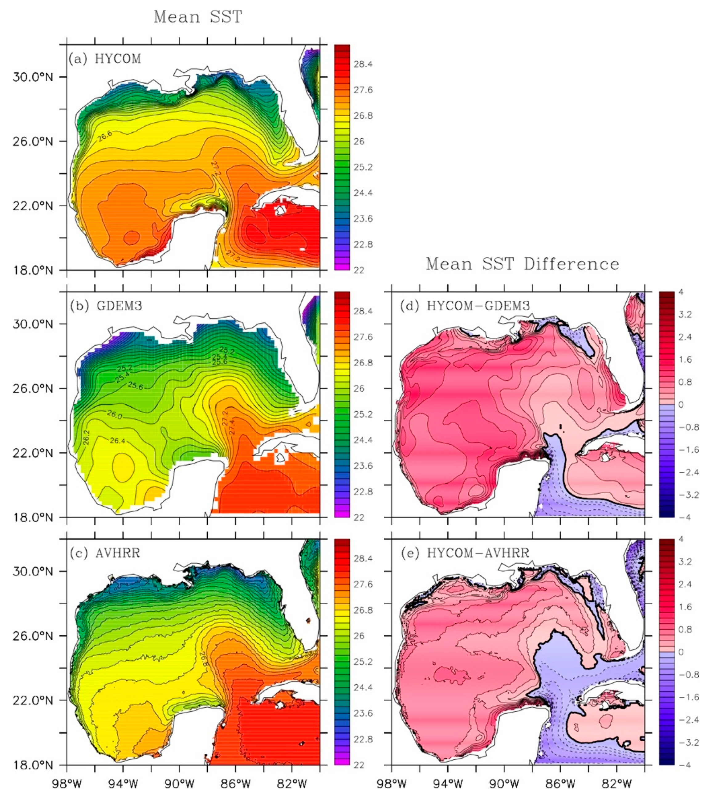
4.1. Mean SST
4.2. Surface Eddy Kinetic Energy
5. Results
5.1. Net Surface Heat Fluxes
5.2. Horizontal Heat Advection
5.3. Vertical Heat Advection
5.4. Eddy Heat Flux Convergence
5.5. Subannual Variability of Heat Terms in the Eddy-Active Region and in the Western GOM
5.6. Heat Budget in Summer and Winter Seasons
6. Summary and Conclusions
Author Contributions
Funding
Institutional Review Board Statement
Informed Consent Statement
Data Availability Statement
Acknowledgments
Conflicts of Interest
Appendix A
References
- Ruiz-Barradas, A.; Nigam, S. Warm season precipitation variability over the U.S. Great Plains in observations, NCEP and ERA-40 reanalyses, and NCAR and NASA atmospheric simulations. J. Clim. 2005, 18, 1808–1830. [Google Scholar] [CrossRef]
- Weaver, S.J.; Nigam, S. Variability of the Great Plains low-level jet: Large-scale circulation context and hydroclimate impacts. J. Clim. 2008, 21, 1521–1551. [Google Scholar] [CrossRef] [Green Version]
- Muñoz, E.; Wang, C.; Enfield, D. The Intra-Americas springtime sea surface temperature anomaly dipole as fingerprint of remote influences. J. Clim. 2010, 23, 43–56. [Google Scholar] [CrossRef] [Green Version]
- Weaver, S.J.; Baxter, S.; Kumar, A. Climatic role of North American low-level jets on U.S. regional tornado activity. J. Clim. 2012, 25, 6666–6683. [Google Scholar] [CrossRef]
- Molina, M.J.; Timmer, R.P.; Allen, J.T. Importance of the Gulf of Mexico as a climate driver for U.S. severe thunderstorm activity. Geophys. Res. Lett. 2016, 43, 12295–12304. [Google Scholar] [CrossRef]
- Morey, S.L.; Bourassa, M.A.; Dukhovskoy, D.S.; O’Brien, J.J. Modeling studies of the upper ocean response to a tropical storm. J. Geophys. Res. 2006, 111, C06029. [Google Scholar] [CrossRef]
- Orusa, T.; Borgogno Mondino, E. Exploring short-term climate change effects on Rangelands and broad-leaved forests by free satellite data in Aosta Valley (Northwest Italy). Climate 2021, 9, 47. [Google Scholar] [CrossRef]
- Liu, J.; Hagan, D.F.T.; Liu, Y. Global land surface temperature change (2003–2017) and its relationship with climate drivers; AIRS, MODIS, and ERA5-Land Based analysis. Remote Sens. 2021, 13, 44. [Google Scholar] [CrossRef]
- Leben, R.R. Altimeter-derived Loop Current metrics. In Circulation in the Gulf of Mexico: Observations and Models; Geophysical Monograph Series; American Geophysical Union: Washington, DC, USA, 2005; Volume 161, pp. 181–201. [Google Scholar] [CrossRef] [Green Version]
- Shay, L.K.; Goni, G.J.; Black, P.G. Effects of a warm oceanic feature on Hurricane Opal. Mon. Wea. Rev. 2000, 128, 1366–1383. [Google Scholar] [CrossRef]
- Scharroo, R.; Smith, W.H.F.; Lillibridge, J.L. Satellite altimetry and the intensification of Hurricane Katrina. In Eos; American Geophysical Union: Washington, DC, USA, 2005; Volume 86. [Google Scholar] [CrossRef] [Green Version]
- Oey, L.-Y.; Ezer, T.; Lee, H.J. Loop Current, rings and related circulation in the Gulf of Mexico: A review of numerical models and future challenges. In Circulation in the Gulf of Mexico: Observations and Models; Geophysical Monograph Series; American Geophysical Union: Washington, DC, USA, 2005; Volume 161, pp. 31–56. [Google Scholar] [CrossRef] [Green Version]
- Oey, L.-Y.; Ezer, T.; Wang, D.-P.; Yin, X.-Q.; Fan, S.-J. Hurricane-induced motions and interaction with ocean currents. Cont. Shelf Res. 2007, 27, 1249–1263. [Google Scholar] [CrossRef]
- Nowlin, W.D.; Mclellan, H.J. A characterization of the Gulf of Mexico waters in winter. J. Mar. Res. 1967, 25, 29–59. [Google Scholar]
- Cochrane, J.D. Separation of an anticyclone and subsequent developments in the Loop Current. In Texas A&M University Oceanography Study; Capurro, L.R.A., Reid, J.L., Eds.; Gulf Publ. Co.: Houston, TX, USA, 1972; Volume 2, pp. 91–106. [Google Scholar]
- Le Hénaff, M.; Kourafalou, V.H.; Morel, Y.; Srinivasan, A. Simulating the dynamics and intensification of cyclonic Loop Current frontal eddies in the Gulf of Mexico. J. Geophys. Res. 2012, 117, C02034. [Google Scholar] [CrossRef]
- Hastenrath, S.L. Estimates of the latent and sensible heat flux for the Caribbean Sea and the Gulf of Mexico. Limnol. Oceanogr. 1968, 13, 322–331. [Google Scholar] [CrossRef]
- Hastenrath, S.L. Heat budget of the Central American Seas. Int. Geophysics. 1976, 16, 117–131. [Google Scholar] [CrossRef]
- Etter, P.C. A Climatic Heat Budget Study of the Gulf of Mexico. Master’s Thesis, Texas A&M University, College Station, TX, USA, 1975. [Google Scholar]
- Etter, P.C. Heat and freshwater budget of the Gulf of Mexico. J. Phys. Oceanogr. 1983, 13, 2058–2069. [Google Scholar] [CrossRef]
- Emery, W.J. The role of vertical motion in the heat budget of the upper Northeastern Pacific Ocean. J. Phys. Oceanogr. 1976, 6, 299–305. [Google Scholar] [CrossRef] [Green Version]
- Vukovich, F.M. Climatology of ocean features in the Gulf of Mexico using satellite remote sensing data. J. Phys. Oceanogr. 2007, 37, 689–707. [Google Scholar] [CrossRef]
- Zavala-Hidalgo, J.; Parès-Sierra, A.; Ochoa, J. Seasonal variability of the temperature and heat fluxes in the Gulf of Mexico. Atmósfera 2002, 15, 81–104. [Google Scholar]
- Change, Y.-L.; Oey, L.-Y. Eddy and wind-forced heat transports in the Gulf of Mexico. J. Phys. Oceanogr. 2010, 40, 2728–2742. [Google Scholar] [CrossRef]
- Rudzin, J.; Morey, S.; Bourassa, M.A.; Smith, S.R. The influence of Loop Current position on winter sea surface temperatures in the Florida Straits. Earth Interact. 2013, 17, 1–9. [Google Scholar] [CrossRef]
- Putrasahan, D.A.; Kamenkovich, L.; Le Henaff, M.; Kirtman, B.P. Importance of ocean mesoscale variability for air-sea interactions in the Gulf of Mexico. Geophys. Res. Lett. 2017, 44, 6352–6362. [Google Scholar] [CrossRef] [Green Version]
- Dukhovskov, D.S.; Leben, R.R.; Chassignet, E.P.; Hall, C.; Morey, S.L.; Nedbor-Gross, R. Characterization of the uncertainty of Loop Current Metrics using a multidecadal numerical simulation and altimeter observations. Deep-Sea Res. 2015, 100, 140–158. [Google Scholar] [CrossRef]
- Nguyen, T.-T.; Morey, S.L.; Dukhovskoy, D.S.; Chassignet, E.P. Non-local impacts of the Loop Current on cross-slope near-bottom flow in the northeastern Gulf of Mexico. Geophys. Res. Lett. 2015, 42, 2926–2933. [Google Scholar] [CrossRef]
- Morey, S.L.; Gopalakrishnan, G.; Sanz, E.P.; De Souza, J.M.A.C.; Donohue, K.; Pérez-Brunius, P.; Dukhovskoy, D.; Chassignet, E.; Cornuelle, B.; Bower, A.; et al. Assessment of numerical simulations of deep circulation and variability in the Gulf of Mexico using recent observations. J. Phys. Oceanogr. 2020, 50, 1045–1064. [Google Scholar] [CrossRef]
- Nedbor-Gross, R.; Dukhovskoy, D.S.; Bourassa, M.A.; Morey, S.L.; Chassignet, E. Investigation of the relationship between the Yucantan Channel transport and the Loop Current area in a multi-decadal numerical simulation. Mar. Technol. Soc. J. 2014, 48, 15–26. [Google Scholar] [CrossRef] [Green Version]
- Halliwell, G.R.; Bleck, R.; Chassignet, E.P. Atlantic Ocean simulations performed using a new hybrid-coordinate ocean model. In Proceedings of the EOS, AGU Fall 1998 Meeting, San Francisco, CA, USA, 6–10 December 1998. [Google Scholar]
- Bleck, R. An oceanic general circulation model framed in hybrid isopycnic-Cartesian coordinates. Ocean. Model. 2002, 4, 55–88. [Google Scholar] [CrossRef]
- Chassignet, E.P.; Smith, L.T.; Halliwell, G.R.; Bleck, R. North Atlantic simulation within the Hybrid Coordinate Ocean Model (HYCOM): Impact of vertical coordinate choice, reference density, and thermobaricity. J. Phys. Oceanogr. 2003, 33, 2504–2526. [Google Scholar] [CrossRef] [Green Version]
- Large, W.G.; McWilliams, J.C.; Doney, S.C. Oceanic vertical mixing: Review and model whith a nonlocal boundary layer parameterization. Rev. Geophys. 1994, 32, 363–403. [Google Scholar] [CrossRef] [Green Version]
- Large, W.G.; Danabasoglu, G.; Doney, S.C.; McWilliams, J.C. Sensitivity to surface forcing and boundary layer mixing in a global ocean model: Annual-mean climatology. J. Phys. Oceanogr. 1997, 27, 2418–2447. [Google Scholar] [CrossRef]
- Carnes, M.R. Description and Evaluation of GDEM-V 3.0; Memorandum Report; US Naval Research Laboratory, Oceanography Division, Stennis Space Center: Hancock County, MS, USA, 2009; Volume 24. [Google Scholar]
- Kilpatrick, K.A.; Podesta, G.P.; Evans, R. Overview of the NOAA/NASA Advanced Very High Resolution Radiometer Pathfinder algorithm for sea surface temperature and associated matchup database. J. Geophys. Res. 2001, 106, 9179–9197. [Google Scholar] [CrossRef]
- Yu, L.; Weller, R.A. Objectively analyzed air–sea heat fluxes for the global ice-free oceans (1981–2005). Bull. Amer. Meteor. Soc. 2007, 88, 527–539. [Google Scholar] [CrossRef] [Green Version]
- Yu, L.; Jin, X.; Weller, R.A. Multidecade Global Flux Datasets from the Objectively Analyzed Air-Sea Fluxes (OAFlux) Project: Latent and Sensible Heat Fluxes, Ocean Evaporation, and Related Surface Meteorological Variables; OAFlux Project Technical Report. OA-2008-01; Woods Hole Oceanographic Institution: Falmouth, MA, USA, 2008; Volume 64. [Google Scholar]
- Saha, S.; Moorthi, S.S.; Pan, H.-L.; Wu, X.; Wang, J.; Nadiga, S.; Tripp, P.; Kistler, R.; Woollen, J.; Behringer, D.; et al. The NCEP climate forecast system reanalysis. Bull. Am. Meteor. Soc. 2010, 91, 1015–1057. [Google Scholar] [CrossRef]
- Rossow, W.B.; Walker, A.W.; Beuschel, D.E.; Roiter, M.D. International Satellite Cloud Climatology Project (ISCCP) documentation of new cloud datasets. In WMO Technical Document 737; WMO: Geneva, Switzerland, 1996; Volume 115. [Google Scholar]
- Zhang, Y.; Rossow, W.B.; Lacis, A.A.; Oinas, V.; Mishchenko, M.I. Calculation of radiative fluxes from the surface to top of atmosphere based on ISCCP and other global data sets: Refinements of the radiative transfer model and the input data. J. Geophys. Res. 2004, 109, D19105. [Google Scholar] [CrossRef] [Green Version]
- Schaeffer, P.; Faugere, Y.; Legeais, J.F.; Picot, N.; Bronner, E. The CNES-CLS11 Global Mean Sea Surface Computed from 16 years of Satellite Altimeter Data. Mar. Geod. 2012, 35, 3–19. [Google Scholar] [CrossRef]
- Johnson, E.S.; Bonjean, F.; Lagerloef, G.S.E.; Gunn, J.T.; Mitchum, G.T. Validation and error analysis of OSCAR sea surface currents. J. Atmos. Oceanic. Technol. 2007, 24, 688–701. [Google Scholar] [CrossRef]
- Talley, L.D.; Pickard, G.L.; Emery, W.J.; Swift, J.H. Mass, Salt, and Heat Budgets and Wind Forcing. In Descriptive Physical Oceanography; Elsevier Ltd.: Amsterdam, The Netherlands, 2011; Volume 560, ISBN 978-0-7506-4552-2. [Google Scholar] [CrossRef]
- Mooers, C. Intra-Americas Circulation. In The Sea, The Global Coastal Ocean, Regional Studies and Syntheses; John Wiley and Sons: Hoboken, NJ, USA, 1998; pp. 183–208. [Google Scholar]
- Nagai, T.; Gruber, N.; Frenzel, H.; Lachkar, Z.; McWilliams, J.C.; Plattner, G.-K. Dominant role of eddies and filaments in the offshore transport of carbon and nutrients in the California Current System. J. Geophys. Res. Oceans 2015, 120, 5318–5341. [Google Scholar] [CrossRef]
- Halliwell, G.R. Diagnosis of Kinematic Vertical Velocity in HYCOM. 2004. Available online: https://www.hycom.org/attachments/067_vertical_vel.pdf (accessed on 17 March 2022).
- Pasqueron de Fommervault, O.; Perez-Brunius, P.; Damien, P.; Camacho-Ibar, V.F.; Sheinbaum, J. Temporal variability of chlorophyll distribution in the Gulf of Mexico: Bio-optical data from profiling floats. Biogeosciences 2017, 14, 5647–5662. [Google Scholar] [CrossRef] [Green Version]
- Hamilton, P.; Leben, R.; Bower, A.; Furey, H.; Pérez-Brunius, P. Hydrography of the Gulf of Mexico Using Autonomous Floats. J. Phys. Oceanogr. 2018, 48, 773–794. [Google Scholar] [CrossRef]
- Meunier, T.; Pallàs-Sanz, E.; Tenreiro, M.; Portela, E.; Ochoa, J.; Ruiz-Angulo, A.; Cusí, S. The Vertical Structure of a Loop Current Eddy. J. Geophys. Res. Oceans 2018, 123, 6070–6090. [Google Scholar] [CrossRef]
- Zavala-Hidalgo, J.; Gallegos-García, A.; Martínez-López, B.; Morey, S.L.; O’Brien, J.J. Seasonal upwelling on the western and southern shelves of the Gulf of Mexico. Oceans Dyn. 2006, 56, 333–338. [Google Scholar] [CrossRef]
- Hamilton, P.; Fargion, G.S.; Biggs, D.C. Loop Current eddy paths in the western Gulf of Mexico. J. Phys. Oceanogr. 1999, 29, 1180–1207. [Google Scholar] [CrossRef]
- Shi, Q.; Bourassa, M.A. Coupling ocean currents and waves with wind stress over the Gulf Stream. Remote Sens. 2019, 11, 1476. [Google Scholar] [CrossRef] [Green Version]
- Gutierrez de Velasco, G.; Winant, C.D. Seasonal patterns of wind stress and wind stress curl over the Gulf of Mexico. J. Geophys. Res. 1996, 101, 18127–18140. [Google Scholar] [CrossRef]
- Elliott, B.A. Anticyclonic rings in the Gulf of Mexico. J. Phys. Oceanogr. 1982, 12, 1292–1309. [Google Scholar] [CrossRef] [Green Version]
- Sturges, W.; Leben, R. Frequency of ring separations from the Loop Current in the Gulf of Mexico: A revised estimate. J. Phys. Oceanogr. 2000, 30, 1814–1819. [Google Scholar] [CrossRef]
- Elliott, B.A. Anticyclonic Rings and the Energetics of the Circulation of the Gulf of Mexico. Ph.D. Thesis, Texas A&M University, College Station, TX, USA, 1979. [Google Scholar]
- Sturges, W. The mean upper-layer flow in the central Gulf of Mexico by a new method. J. Phys. Oceanogr. 2016, 46, 2915–2924. [Google Scholar] [CrossRef]
- Portela, E.; Tenreiro, M.; Pallàs-Sanz, E.; Meunier, T.; Ruiz-Angulo, A.; Sosa-Gutiérrez, R.; Cusí, S. Hydrography of the central and western Gulf of Mexico. J. Geophys. Res. Oceans 2018, 123, 5134–5149. [Google Scholar] [CrossRef]
- Colbo, K.; Weller, R. The variability and heat budget of the upper ocean under the Chile-Peru stratus. J. Marine. Res. 2007, 65, 607–637. [Google Scholar] [CrossRef]
- Simonot, J.-Y.; Le Treut, H. A climatological field of mean optical properties of the world ocean. J. Geophys. Res. 1986, 91, 6643–6646. [Google Scholar] [CrossRef]
- Kara, A.B.; Wallcraft, A.J.; Hurlburt, H.E. A new solar radiation penetration scheme for use in ocean mixed layer studies: An application to the black sea using a fine-resolution hybrid coordinate ocean model (HYCOM). J. Phys. Oceanogr. 2005, 35, 13–32. [Google Scholar] [CrossRef] [Green Version]


| Variables | Dataset | Spatial Coverage/Grid Spacing (o) | Temporal Coverage | References |
|---|---|---|---|---|
| SST | AVHRR | Global ocean 9 km × 9 km | January 1985–December 2002 | [37] |
| Ocean temp | HYCOM GDEM3 | GOM 1/25 × 1/25-L40 Global ocean 0.25 × 0.25-L78 | 54 years climatology | [27] [36] |
| Ocean velocity | HYCOM | Global ocean 1/25 × 1/25-L40 | 54 years | [27] |
| Ocean surf velocity | AVISO OSCAR | Global ocean 1/3 × 1/3 Global ocean 1/3 × 1/3 | January 1993–December 2014 January 1993–December 2014 | [43] [44] |
| Sea surf height | HYCOM | GOM 1/25 × 1/25-L40 | January 1993–December 2012 | [27] |
| Net surf heat flux | OAFlux | Global ocean 1 × 1 | July 1983–December 2009 | [38] |
| Surf latent/sensible heat flux | HYCOM CFSR | GOM 1/25 × 1/25-L40 Global ocean 1 × 1 | 54 years January 1979–December 2009 | [27] [40] |
| Net surf shortwave/longwave flux | ISCCP-FD | Global ocean 1 × 1 | July 1983–December 2007 | [41] |
| Regions | hsr | Qnet | advh | advgeo | advageo | advz | eddyh | eddyz | Residual |
|---|---|---|---|---|---|---|---|---|---|
| EDDY | |||||||||
| WGOM |
| JJA | |||||||||
| Regions | hsr | Qnet | advh | advgeo | advageo | advz | eddyh | eddyz | Residual |
| EDDY | 80.6 | 65.5 | −50.6 | −33.2 | −17.4 | 90.2 | −2.1 | 6.8 | −29.2 |
| WGOM | 74.7 | 68.1 | 14.7 | 6.5 | 8.2 | −2.0 | −2.9 | 5.8 | −9.0 |
| DJF | |||||||||
| Regions | hsr | Qnet | advh | advgeo | advageo | advz | eddyh | eddyz | Residual |
| EDDY | −91.3 | −115.0 | 3.5 | −1.1 | 4.6 | 105.5 | −15.6 | 5.6 | −75.3 |
| WGOM | −94.5 | −103.3 | 19.3 | 9.4 | 9.9 | −11.6 | −1.9 | 6.6 | −3.6 |
Publisher’s Note: MDPI stays neutral with regard to jurisdictional claims in published maps and institutional affiliations. |
© 2022 by the authors. Licensee MDPI, Basel, Switzerland. This article is an open access article distributed under the terms and conditions of the Creative Commons Attribution (CC BY) license (https://creativecommons.org/licenses/by/4.0/).
Share and Cite
Zheng, Y.; Bourassa, M.A.; Dukhovskoy, D.; Ali, M.M. Upper-Ocean Processes Controlling the Near-Surface Temperature in the Western Gulf of Mexico from a Multidecadal Numerical Simulation. Earth 2022, 3, 493-521. https://doi.org/10.3390/earth3020030
Zheng Y, Bourassa MA, Dukhovskoy D, Ali MM. Upper-Ocean Processes Controlling the Near-Surface Temperature in the Western Gulf of Mexico from a Multidecadal Numerical Simulation. Earth. 2022; 3(2):493-521. https://doi.org/10.3390/earth3020030
Chicago/Turabian StyleZheng, Yangxing, Mark A. Bourassa, Dmitry Dukhovskoy, and M. M. Ali. 2022. "Upper-Ocean Processes Controlling the Near-Surface Temperature in the Western Gulf of Mexico from a Multidecadal Numerical Simulation" Earth 3, no. 2: 493-521. https://doi.org/10.3390/earth3020030