Evaluation of Three Reanalysis Soil Temperature Datasets with Observation Data over China

Abstract

Soil temperature is a crucial parameter in surface emissions of carbon, water, and energy exchanges. This study utilized the soil temperature of 836 national basic meteorological observing stations over China to evaluate three soil temperature products. Soil temperature data from the China Meteorology Administration Land Data Assimilation System (CLDAS), European Centre for Medium-Range Weather Forecasts (ERA-Interim), and Global Land Data Assimilation System (GLDAS) during 2017 are evaluated. The results showed that soil temperature reanalysis datasets display a significant north-to-south difference over eastern China with generally underestimated magnitudes. CLDAS data perform soil temperature assessment best at different depths and can be reproduced well in most areas of China. CLDAS slightly overestimates soil temperature in summer. The most significant deviation of ERA-Interim (GLDAS) appears in summer (summer and autumn). As soil depth increases, the soil temperature errors of all three datasets increase. The CLDAS represents the soil temperature over China but owns a more considerable bias in barren or sparsely vegetated croplands. ERA-Interim performs poorest in urban and built-up and barren or sparsely vegetated areas. GLDAS overall owns an enormous bias at the mixed forest, grassland, and croplands areas, which should be improved, especially in summer. However, it performs better in open shrublands and barren or sparsely vegetated areas. The ST of mixed forests shows better results in the south region than the north region. For grasslands, smaller MEs are located in the north and northwest regions. The ST of croplands shows the poorest performance over the northwest region.

1. Introduction

Soil temperature (ST) is an essential parameter that can affect exchanges of heat flux between the atmosphere and land surface [1,2], further affecting regional weather and climate [3,4]. Variations in ST alter the partition of sensible and latent heat flux at the surface, influencing the boundary layer processes and regional and global circulation [5,6]. To better research the regional climate characteristics, it is vital to figure out ST’s spatial distribution and annual variation. Many factors, such as air temperature, precipitation, vegetation, and solar radiation, affect ST [7,8,9]. Between-model differences can be traced to differences in the coupling between either near-surface air and shallow soil temperatures or shallow and deeper soil temperatures, which reflect differences in snow physics and soil hydrology [10,11].

ST’s spatial distribution and variations can be directly observed through in situ observation stations [12,13]. Yang and Zhang [14] illustrated that the soil temperature memory over China represents a similar northwest-to-southeast gradient spatial pattern over China. Zhu et al. [15] showed that the Plateau has experienced a significant warming trend. However, the heterogeneity of ST is substantially affected by topography, land cover, and vegetation [16,17]. Direct observations of ST have higher accuracy. However, the limitation of the spatial and temporal distribution of observation sites still cannot be ignored, especially in northwest China and on the Qinghai–Tibet Plateau. Other high-resolution products, such as model results [18,19] and satellite remote sensing data [20], are needed to supplement incomplete observations.

Numerous numerical model results and reanalysis data provide high-resolution soil temperature data (ERA-Interim, CFSR, CFSv2, JRA-55, GLDAS, etc.) [21,22]. These datasets have been widely applied in climatology research, and their reliability has been evaluated. Betts et al. [23] illustrated that ERA-40 data represents the climatological ST gradient of the Mackenzie Basin well. Robock et al. [24] showed that North American Land Data Assimilation System soil temperature products fit well with observations. Wang et al. [25] found that the GLDAS_CLM made an overestimation, while GLDAS_NOAH was the reverse. Yang and Zhang [14] evaluated the soil temperature the land surface reanalysis of the ECWMF (ERA-Interim/land), the second modern-era retrospective analysis for research and applications (MERRA-2), the National Centre for Environmental Prediction Climate Forecast System Reanalysis (NCEP-CFSR), and version 2 of the Global Land Data Assimilation System (GLDAS-2.0) over China. They found that reanalysis data can mainly reproduce the spatial distributions of soil temperature in summer and winter, especially over eastern China. Qin et al. [26] illustrated that three reanalysis ST products underestimate observations with negative mean bias error values at all three soil layers. The MERRA-2 product performed best in the first and second soil layers, and the ERA-Interim product performed best in the third. Xue et al. [27] found that CFSR dramatically underestimated soil temperature in July 2013. Generally speaking, no one product shows the best performance in all regions. However, most assessment research mainly focuses on reanalysis datasets from the United States or Europe [28,29]. Evaluations of soil temperature data from Chinese products are still scarce. Meanwhile, China’s climate differs across its vast territory because of the differences in altitude, elevation, and ocean distances [30]. Different evaluations are shown in other parts of China, so the reliability of reanalysis data applied to China also needs further investigation. The statistical results of Yang et al. [31] illustrated that GLDAS-Noah products ranked at the top of the four products in simulating soil temperature, especially in the alpine desert, alpine swamp, and alpine grassy meadow. In addition, the ERA-Interim product was superior to the other products in simulating soil moisture in permafrost regions on the QTP, especially in the alpine desert and alpine meadow. Additionally, the ERA5 product was better than ERA-Interim in simulating soil temperature, especially topsoil. Still, it did not perform superiorly in simulating soil moisture in permafrost regions of the QTP, which may be related to the different land surface models and soil texture between the two products.

The accuracy of and applicability of three soil temperature datasets over major land areas of China are evaluated. The reproductivity skills of the reanalysis dataset in different elevations and land use are assessed. Observed ST data of ground weather stations are utilized to evaluate. China Meteorology Administration (CMA) Land Data Assimilation System (CLDAS), land surface reanalysis of the European Centre for Medium-Range Weather Forecasts (ERA-Interim), and version 2.1 of Global Land Data Assimilation System (GLDAS-v2.1) are evaluated in this study. Among the soil temperature observations we have obtained, after quality control, there are fewer missing values in 2017, so we chose 2017 as the research period. The evaluation results can help researchers improve and innovate these datasets in different land cover categories. Moreover, it will provide suggestions for selecting appropriate datasets for climate change research and model improvement.

Data and methods are described in Section 2. The results of the assessment are presented in Section 3. Section 4 provides a brief discussion and summary of the relevant results.

2. Data and Methods

2.1. Observations

The monthly mean ST of different layers observed by national basic meteorological observing stations is assessed. The observation data have been verified by checking the climatological threshold value, regional, temporal, and spatial consistency. After data quality control, soil temperature data of 836 stations in 2017 were chosen to evaluate three reanalysis datasets. The observation data contain nine layers, including soil temperature at 5, 10, 15, 20, 40, 80, 160, and 320 cm depths. Soil temperatures at 10 cm (ST10), 20 cm (ST20), 40 cm (ST40), and 80 cm (ST80) were utilized in this study.

The spatial distribution of the observed stations of different elevations is shown in Figure 1a. According to the elevation of observed stations, the 836 stations were divided into four categories, including elevations less than 1000 m (E1, 568 stations, gray), between 1000 m and 2000 m (E2, 164 stations, light-blue), between 2000 m and 3000 m (E3, 40 stations, pink), and greater than 3000 m (E4, 64 stations, purple). The observation stations are densely distributed in central and south China and sparsely distributed in the northwest and Tibetan Plateau regions.

According to China’s geographical division [32], observed stations are divided into four geographic regions (Figure 1b), including the north region (276 stations, red), south region (348 stations, green), northwest region (136 stations, golden), and Tibetan region (76 stations, blue). The observation stations are densely distributed in north and south China and sparsely distributed in the northwest and Tibetan region.

According to the International Geosphere-Biosphere Program (IGBP), land-use data derived from remote sensing data and observed stations’ land-use were classified. The counts and percentages of different land-use categories are listed in

Table 1. The counts and percentages of observation stations at different land-use.

Value	Land Use Type	Counts	Percent (%)
1	Evergreen Needleleaf Forest	0	0
2	Evergreen Broadleaf Forest	24	2.87
3	Deciduous Needleleaf Forest	0	0
4	Deciduous Broadleaf Forest	1	0.12
5	Mixed Forests	162	19.38
6	Closed Shrublands	0	0
7	Open Shrublands	5	0.6
8	Woody Savannas	57	6.82
9	Savannas	0	0
10	Grasslands	205	24.52
11	Permanent Wetlands	1	0.12
12	Croplands	260	30.1
13	Urban and Built-up	4	0.48
14	Crop/Natural Vegetation Mosaic	35	4.19
15	Snow and Ice	0	0
16	Barren or Sparsely Vegetated	54	6.46
17	Water Bodies	28	3.35

. The croplands (30.1%), grasslands (24.5%), and mixed forests (19.4%) took a more significant proportion.

2.2. CLDAS

The CLDAS dataset is developed by CMA, which covers the east Asian Region (0–60° N, 70–150° E) [33]. Soil temperatures at 10, 40, 100, and 200 cm are provided in CLDAS. The spatial resolution is 0.0625° × 0.0625°, and the temporal resolution is 1 h. The Community Land Model (CLM) produces the CLDAS soil temperature. Hourly gridded forcing data, including air temperature, pressure, humidity, wind speed, downward shortwave radiation, and precipitation, are used to drive CLM in CLDAS. Regional automatic surface observation temperatures (over 30,000) over China are combined with NCEP/GFS data by Space-Time Multi-Scale Analysis System.

2.3. ERA-Interim

ERA-Interim is the latest global atmospheric reanalysis produced by the European Centre for Medium-Range Weather Forecasts (ECMWF) [34]. ERA-Interim provides a dataset from 1989 to a near-real-time dataset. This product is based on a data assimilation system that assimilates various observations, including satellites and ground-based observations, in a consistent framework. An optimal interpolation scheme produces 6-h estimates of screen-level temperature. The analysis increments for screen-level temperature and humidity are subsequently employed to update soil temperature estimates for each of the four layers of the land-surface model. The soil temperature data of ERA-Interim contain four soil layers (0–7, 7–28, 28–100, and 100–189 cm). In this study, the monthly mean monthly soil temperature of 0–7, 7–28, and 28–100 cm were assessed, and the spatial resolution was 0.125° × 0.125°.

2.4. GLDAS-2.1

GLDAS is developed by scientists of the National Aeronautics and Space Administration, Goddard Space Flight Center, the National Oceanic and Atmospheric Administration, and NCEP [35]. GLDAS aims to ingest satellite- and ground-based observational data products using advanced land surface modeling (Land Information System, LIS) and data assimilation techniques to generate optimal fields of land surface states and fluxes. The Noah Land Surface Model was developed to operate and research NCEP weather and climate models, and it continues to benefit from a steady progression of improvements. This dataset provides data ranging from 2000 to almost real-time. The GLDAS soil temperature data contain four levels: 0–10, 10–40, 40–100, and 100–200 cm. Soil temperatures of 0–10, 10–40, and 40–100 cm with a spatial resolution of 0.25° × 0.25° were used in this study.

Inconsistencies between the observed and reanalysis data of soil depths exist. The reanalysis data were interpolated to the observational depths with the soil thicknesses as weights [36]. The vertical variation in observed ST is approximately linear, especially for the soil temperature at 0–40 cm depth. Linear interpolation was used to interpolate reanalysis data.

2.5. Measures of the Performance

Soil temperature datasets were compared with the corresponding soil temperature observations. A variety of statistical methods are available for soil temperature evaluation. In this study, the following statistical methods for error analysis were used. The correlation coefficient (R), mean error (ME), and root-mean-square error (RMSE) were used to quantify differences between the soil temperature reanalysis products and in situ observations.

2.5.1. Mean Error

$$ME=\frac{1}{n}{\displaystyle \sum _{i=1}^n(F_i-O_i)}$$

(1)

where n is the number of samples (specifically, n is the number of observation stations), F_i (O_i) is the simulation (observation) value of station i.

The mean error (ME) represents the difference between the reanalysis data for all observation stations and the corresponding observed values.

2.5.2. Absolute Mean Error

$$MAE=\frac{1}{n}{\displaystyle \sum _{i=1}^n\left|(F_i-O_i)\right|}$$

(2)

The absolute mean error (MAE) represents the average distance between observation stations and the corresponding observed values.

2.5.3. Root-Mean-Square-Error

The root-mean-square error (RMSE) measures accuracy in comparing the errors of different models for a particular dataset.

$$RMSE=\sqrt{\frac{1}{n}{\displaystyle \sum _{i=1}^n{(F_i-O_i)}^2}}$$

(3)

RMSE represents the square root of the ratio of the summed squared deviations of the reanalysis data for all observation stations and the corresponding observed values relative to the number of observation stations.

3. Results

3.1. Spatial Distributions of the Annual Average of Different Elevations

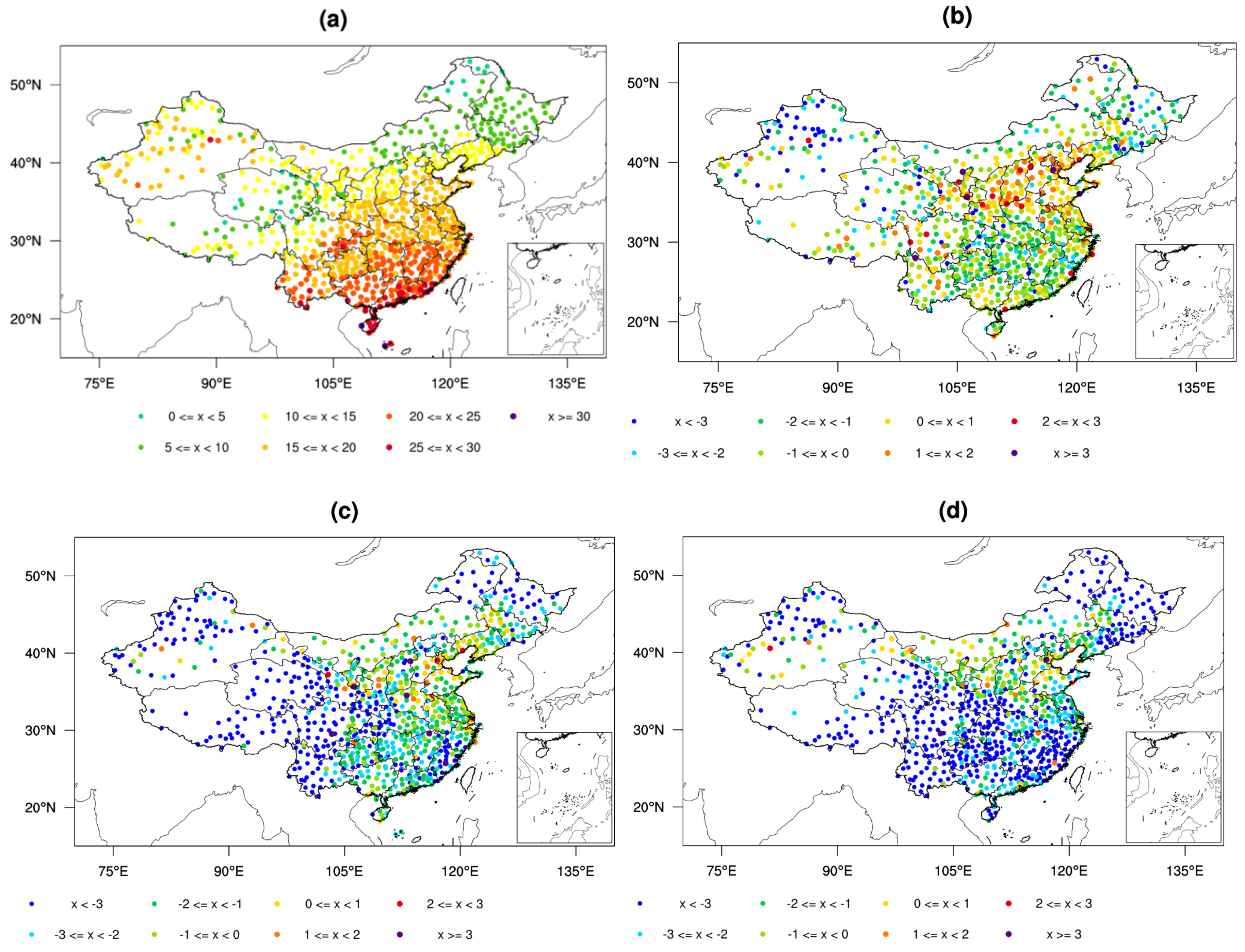
First, we evaluate the ability of the different datasets to represent the spatial distribution of soil temperature during 2017. The spatial distributions of observations (OBS) and ME of ST10 (averaged results of one year) are shown in Figure 2.

The averaged ST10 observations (Figure 2a) of 2017 are above 0 °C, displaying a significant north-to-south difference over China. ST10 is relatively high in the south and low in north China and the Tibetan Plateau. Soil temperature ME of CLDAS (Figure 2b) illustrates that CLDAS mainly underestimated ST10, mainly between −2 and 1 °C. Positive biases appear over north China; the most significant underestimation occurred in northwest China. Spatial distributions of ERA-Interim (Figure 2c) are similar to CLDAS but with a more considerable bias. The number of stations with an error exceeding −3 °C significantly increased. The GLDAS (Figure 2d) data almost all significantly underestimate ST10 (exceeding −3 °C).

Although three products underestimate ST10, they generally capture the spatial distribution of ST10 over China. The spatial distributions of soil temperature in the CLDAS and GLDAS datasets have more in common with the observations. Overall, the CLDAS data reflect ST10 well in most areas of China.

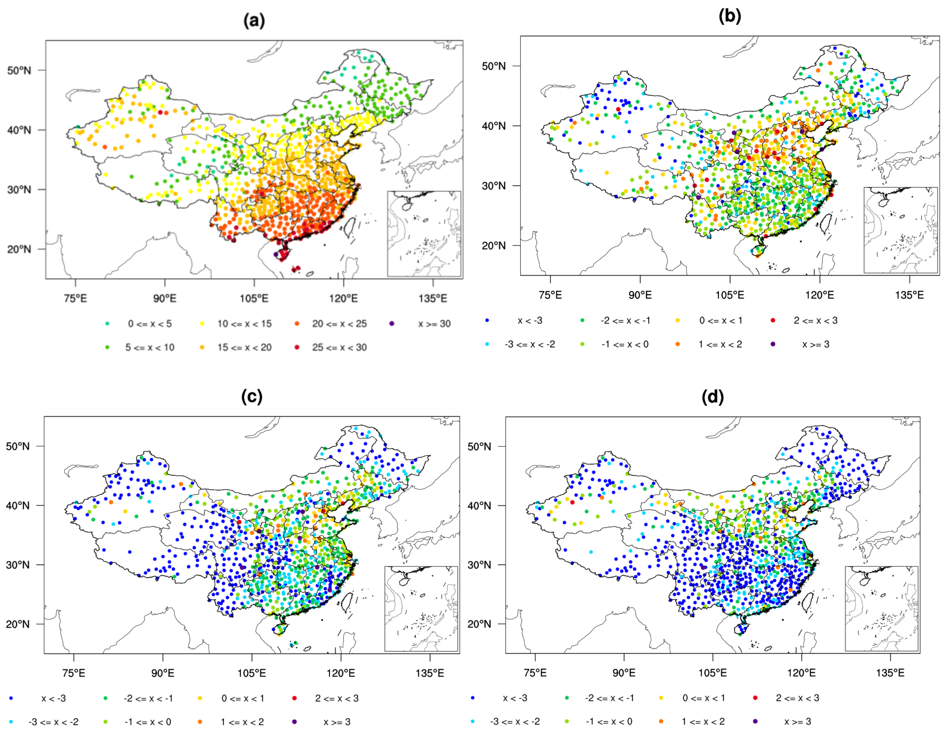
Variations in soil temperature from different layers are the results of complex processes. Like ST10, soil temperature observations at 20 cm (ST20) also represent a distinct temperature gradient from north-to-south over eastern China (Figure 1a). The CLDAS dataset (Figure 2b) can mainly capture the soil temperature distribution over China. Except for stations in eastern China, ERA-interim (Figure 3c) underestimates soil temperature at almost all stations. The GLDAS (Figure 4d) shows the most considerable underestimation in most areas of China. Three reanalysis datasets can represent ST20 in north China. Overall, the CLDAS shows a minor bias of averaged soil temperature. The underestimation of the soil temperature at 20 cm of GLDAS is the largest.

Compared to ST10 (shown in Figure 2), ST20 (Figure 3) in CLDAS shows a smaller positive bias. It should be noted that the ERA-Interim delivers better performance in some stations in northern and southern China. The ERA-Interim dataset captures the spatial characteristics of the observations over central China and south China, but they do not rebuild the ST20 spatial patterns in western China. Except for ST20 in north China, the underestimations of soil temperature in GLDAS are almost larger than 2 °C. For ST20, the CLDAS dataset still performs best among the three datasets, followed by ERA-Interim. GLDAS has the most considerable bias among the three reanalysis datasets at ST20.

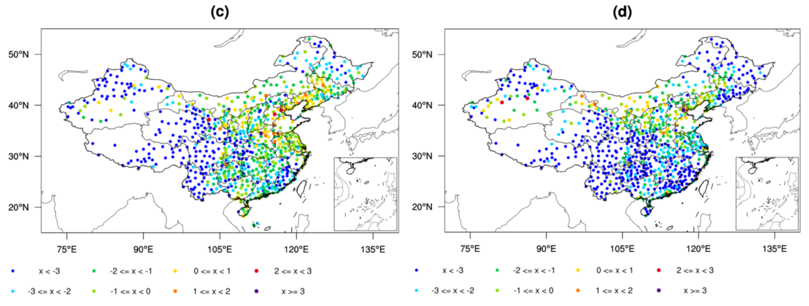
The spatial distributions of the soil temperature at 40 cm and 80 cm (ST40 and ST80; Figure 4 and Figure 5) are similar to ST20 (Figure 3) but with a lower value. The northeast of China and the Tibetan Plateau are lower than 0 °C. The absolute value of the ME of CLDAS, greater than 3 °C, is the lowest. GLDAS also owes the largest negative biases.

To quantify the differences between ST products and the observed ST of different depths over China, the correlation coefficient (R), mean error (ME), and root mean square error (RMSE) are listed in Table 1. The correlation coefficient (R) gives a more accurate representation of the degree and direction of correlation between simulations and observations. As is shown in

Table 2. Correlation coefficient (R), mean error (ME), and root-mean-square error (RMSE) of soil temperature.

		ST10	ST20	ST40	ST80
R	CLDAS	0.88 *	0.89 *	0.88 *	0.88*
	ERA-Interim	0.81 *	0.82 *	0.81 *	0.81 *
	GLDAS	0.75 *	0.75 *	0.77 *	0.76 *
ME/(°C)	CLDAS	−0.52	−0.56	−0.35	−0.56
	ERA-Interim	−1.10	−2.29	−1.99	−2.04
	GLDAS	−2.91	−3.09	−2.88	−3.00
RMSE/(°C)	CLDAS	1.39	1.41	1.38	1.46
	ERA-Interim	2.33	3.07	2.86	2.90
	GLDAS	3.60	3.75	3.57	3.66

* indicates the significance level of 0.05.

, soil temperature’s correlation coefficients of different layers from all three reanalysis datasets reach the 0.05 significance level. The correlation among reanalysis data showed that the soil temperature of CLDAS is larger than 0.85, and the GLDAS correlation is minimal (about 0.75), which has no difference among different soil layers in each dataset. The ME between reanalysis data and OBS is all negative, consistent with the previous regional distribution results. The three reanalysis products all underestimate the soil temperature at different soil depths. The smallest negative bias of CLDAS is −0.35 at 40 cm, and the largest bias (−3.09 °C) is GLDAS at ST40. RMSE shows the same statistical characteristics as ME. The CLDAS dataset shows the smallest ME of one-year averaged results compared to the other datasets in terms of R, ME, and RMSE.

3.2. Monthly Characteristics

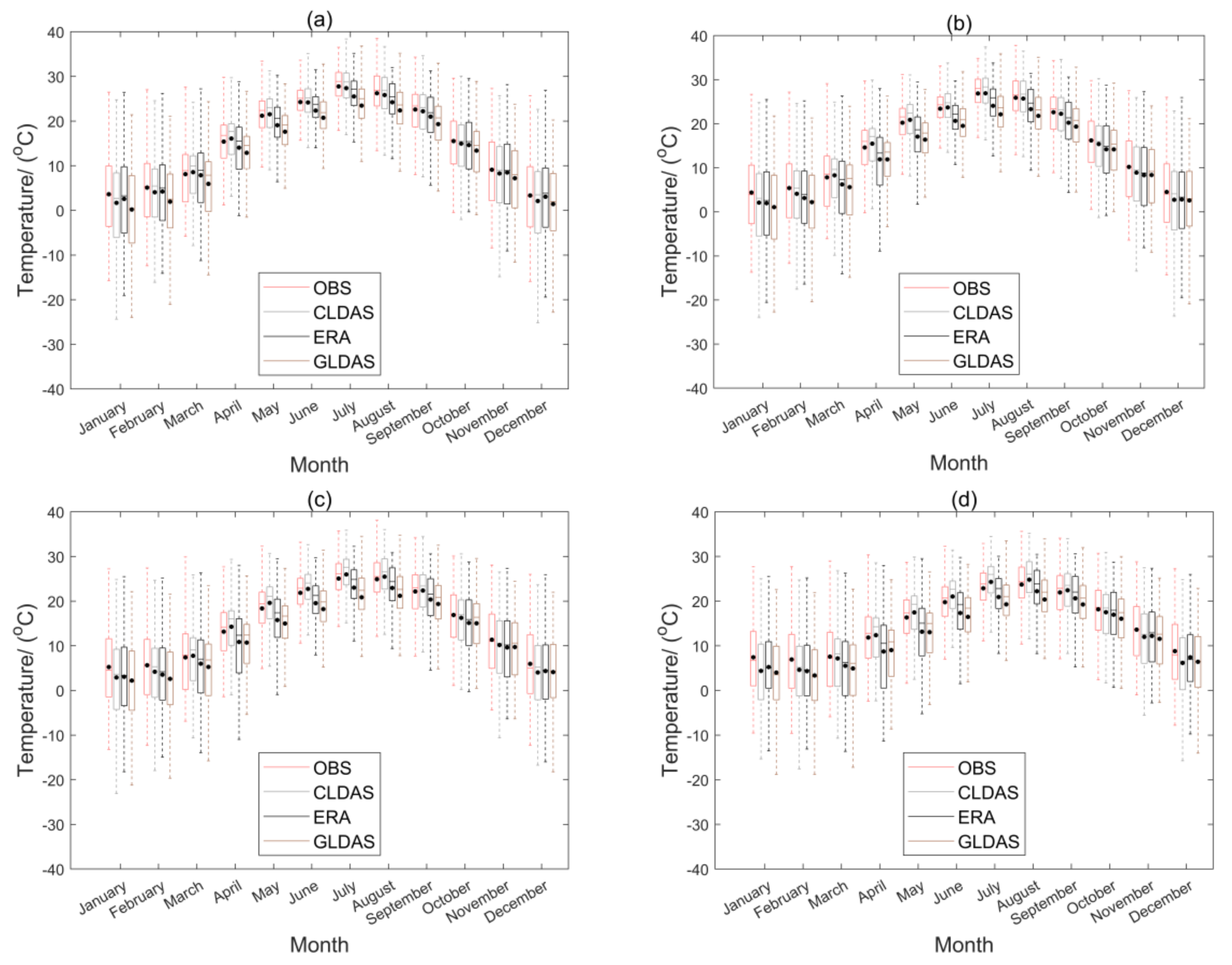
Monthly characteristics of soil temperature and in situ observations of all stations over China in 2017 are also evaluated (Figure 6). The observed ST10 increases from January, peaks in July, and decreases gradually. Three products all underestimate ST10 but with varying magnitudes. The apparent underestimation period is winter in CLDAS, winter and spring in GLDAS, and May to September in ERA-Interim. The reason for these results may be related to the applicability of parameterization schemes in different seasons.

Observed soil temperature changes in ST20 and ST40 are similar to ST10, except for smaller maximum values. CLDAS slightly overestimate ST10 in summer. ERA-Interim (GLDAS) significantly underestimated ST20 and ST40 in spring (summer), especially in April (July). Unlike other depths, observed ST80 rises from March and peaks in August. The three reanalysis datasets captured these characteristics. However, larger underestimations appeared in the spring and summer of ERA-Interim and GLDAS.

3.3. Biases of Different Elevations

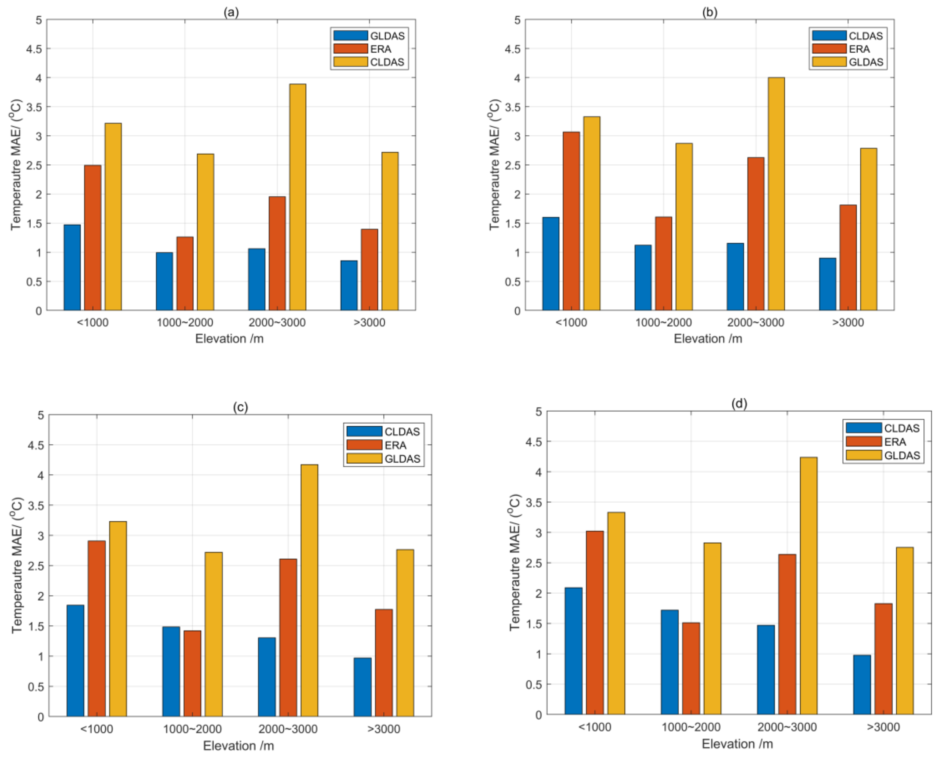
Similar to air temperature, soil temperature is definitely influenced by elevation. The MAE of CLDAS ST10 is mainly below 1.5 °C. With the increase in elevation, the error of ST10 shows different characteristics (Figure 7a). The MAE of CLDAS decreases with the rise in elevation. However, the MAEs of ERA-Interim and GLDADS are the smallest at an elevation between 1000 and 2000 m. The MAEs of ST20 (Figure 7b) are similar to ST10. Variations in ST40′s MAEs (Figure 7c) and ST80′s MAEs (Figure 7d) have similar trends but larger values.

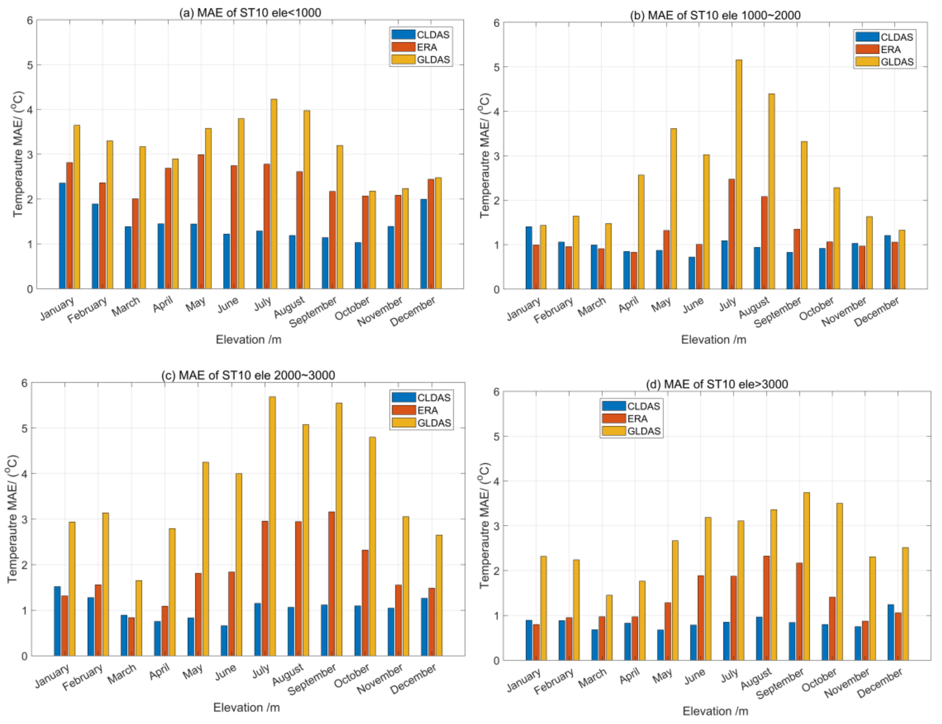
Monthly variations in ST10 (Figure 6) show differences between the three datasets. Monthly results of ST10′s MAE with the elevation below 1000 m (Figure 8a) illustrated that CLADS shows a “U” pattern, with maximum bias in October (1 °C). The trends of ERA-Interim and GLDAS are similar but with a more significant bias in GLDAS. It should be noted that GLADS owes an enormous bias in summer (approximately 4 °C). With the elevation at 1000–2000 m (Figure 8b), the MAE of CLADS has no significant difference in other months (approximately 1 °C). Except for July and August, ERA-Interim’s MAE is below 1.5 °C. GLDAS’s MAE represents an inverted “U” pattern, with a maximum bias larger than 5 °C. Compared to 1000–2000 m (Figure 8b), the MAE at the elevation of 2000–3000 m (Figure 8c) represents more remarkable differences. CLDAS’s MAEs are slightly larger at 1000–2000 m. ERA-Interim and GLDAS show a similar trend but a much larger bias, especially the GLDAS’s MAEs from July to October. Air temperature and precipitation may be the main influencing factors of summer ST10. MAEs at an elevation larger than 3000 m (Figure 8d) show the slightest bias at different elevations.

With the increase in elevation, the bias of CLDAS shows a decreasing trend, with the largest bias being at elevation less than 1000 m. The bias is less than 1 °C at elevations larger than 3000 m. The bias of ERA-Interim data also shows a decreasing trend with elevation trend, but with a larger bias in summer at an elevation between 2000 and 3000 m. Interestingly, the errors of CLDAS are significantly larger from May to October than in other months.

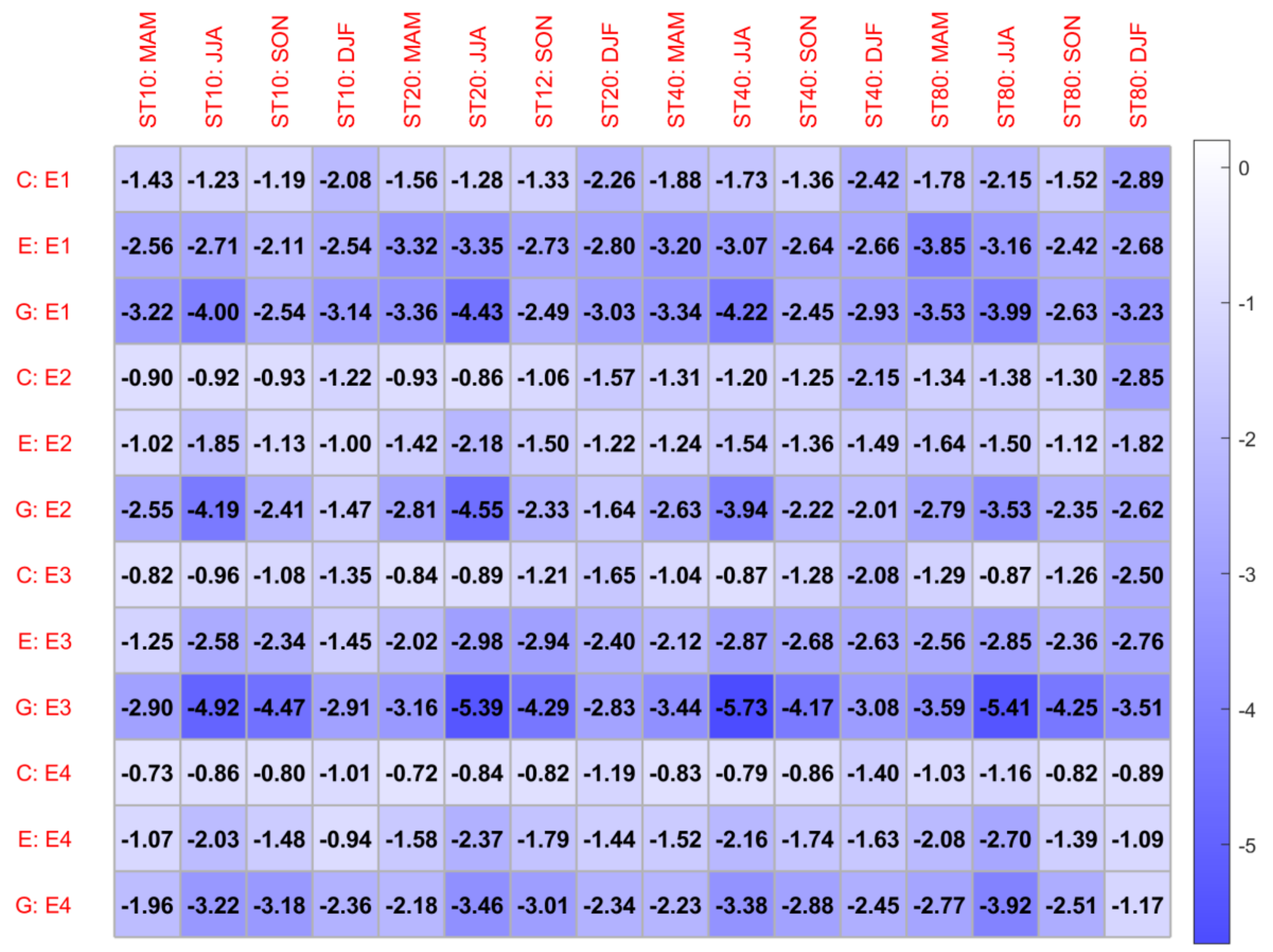
To better understand seasonal variations, the MEs of different datasets are shown in Figure 9. With elevation < 1000 (E1), CLDAS shows the most significant bias in winter at all soil depths. It represents soil temperature relatively better in autumn. ERA-Interim’s MEs are significantly larger in spring and summer than in other seasons. The MEs of GLDAS is the largest in summer, with maximum bias in ST20 (−4.4 °C). The ME of GLDAS at E1 is obviously larger than CLDAS and ERA-Interim.

For elevation between 1000 and 2000 m (E2), except in the summer of GLDAS, the MAE values are all lower than E1. The ERA-Interim’s ME is significantly the smallest in ST40 and ST80 in autumn and winter. With elevation between 2000 and 3000 m (E3), CLDAS has poor winter performance at ST40 and ST80. It should be noted that GLDAS’s ME reached 5.73 °C in summer, deviating from observation. At elevation >3000 m (E4), except in the winter of ST10, CLDAS performs best at all soil depths. Overall, GLDAS’s ME is relatively more minor than other elevations.

Overall, the CLDAS performs best at different depths. The most significant bias of ERA-Interim appeared in summer, with a larger value in lower elevation stations. The GLDAS’s soil temperature performs poorest in summer and autumn. As the soil depth increases, the change in soil temperature is constantly growing.

3.4. Biases of Different Land-Use

Except for the elevation of observed stations, land-use also affects soil temperature [1]. The soil temperature bias over different land use is shown in Figure 9. When soil depths increase, the negative deviation increases with mixed forest (category 5 accounts for 19.38%). Crop/natural vegetation mosaic (category 14 accounts for 4.19%) and barren or sparsely vegetated (category 16 accounts for 6.46%) are more extensive than other categories.

ERA-Interim performs poorest in urban and built-up areas. GLDAS has the most significant bias but performs better in open shrublands and barren or sparsely vegetated areas.

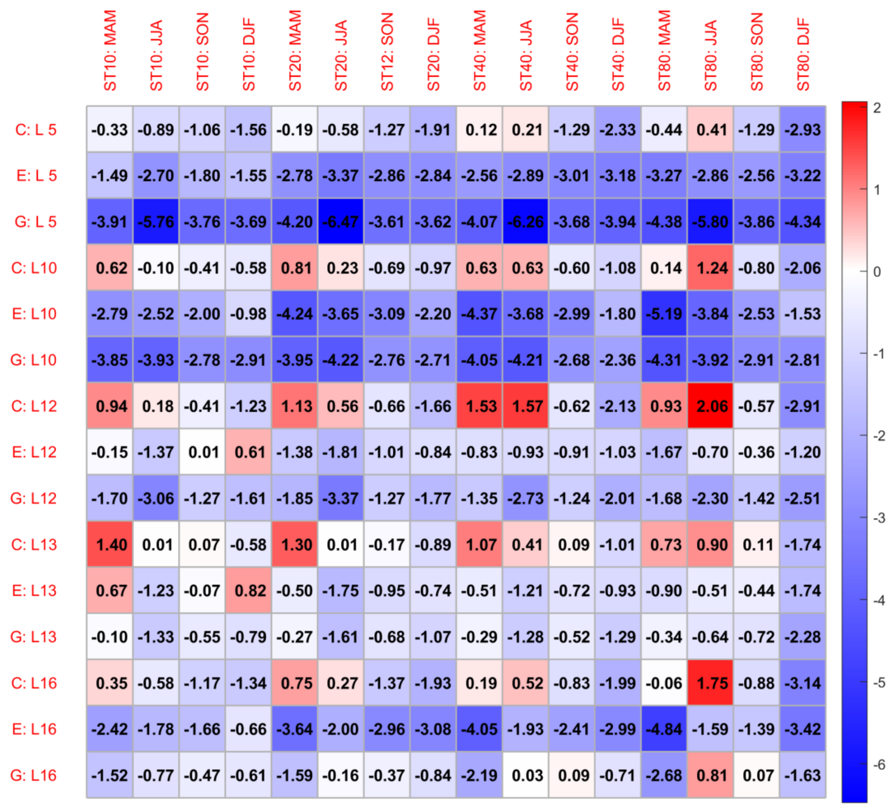
According to the characteristics of ME (Figure 10) and proportions of different categories, seasonal ME variations in mixed forest (L5), grasslands (L10), croplands (L12), urban and built-up land (L13), and barren or sparsely vegetated land (L16) are shown in Figure 11. Like the characteristics of different elevations, ME also represents remarkable seasonal variations in land use. Compared to other land uses, the biases of mixed forests are relatively larger. CLDAS and ERA-Interim perform better in spring. For grassland, CLDAS underestimates ST in spring and summer. However, ERA-Interim and GLDAS significantly overestimate ST, especially in spring and summer. As to croplands, ERA-Interim performs much better than the other two datasets. It is worth analyzing the underlying urban build-up, which has particular thermal and dynamic characteristics. It should be noted that GLDAS has the smallest bias (smaller than 0.5 °C) in spring at different layers and performs better in ST10 and ST20 at all seasons. Concerning barren and sparsely vegetated land, except for in spring, GLDAS performs the best, and then CLDAS.

The representation of GLDAS in the mixed forest, grassland, and croplands should be improved, especially in summer. Meanwhile, CLDAS and ERA-Interim perform well in the mixed forest, grasslands, and croplands. Generally, the performances of ST data of CLDAS and GLDAS in urban and built-up areas need to be improved in spring and summer, respectively. GLDAS has the largest bias overall, but it performs better in open shrublands and barren or sparsely vegetated areas.

3.5. Biases of Different Land Use over Different Regions

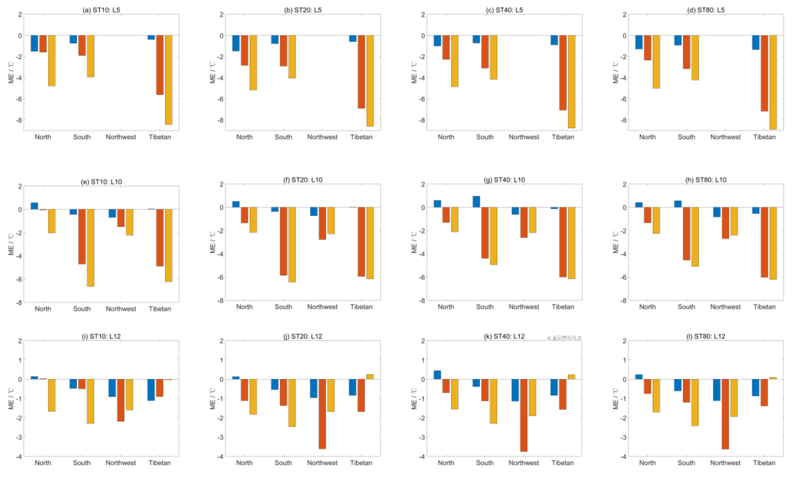
Croplands (category 12, 30.1%), grasslands (category 10, 24.5%), and mixed forests (category 5, 19.4%) make up the largest part of observed stations, accounting for 74.0%. The ST of the same land cover category may behave differently in different regions due to climate conditions. These three land cover categories are analyzed in different regions. The station numbers in four regions are listed in

Table 3. The counts and percentages of observation stations at different regions of mixed forests, grassland, and cropland.

	North	South	Northwest	Tibetan
Mixed forests (L5)	46	113	0	3
Grasslands (L10)	57	4	83	61
Croplands (L12)	149	105	4	2

. Mixed forests are mainly distributed in the south and north regions.

Meanwhile, grasslands are mainly located in the northwest region. The north and Tibetan Plateau have a similar number of grasslands stations. Like mixed forests, croplands are mainly located in the north and south regions.

The MEs of ST in different regions are further analyzed in mixed forests, grassland, and croplands. The MEs vary significantly across different regions.

MEs show similar characteristics in different regions for the ST of mixed forests (Figure 12a–d) at four soil depths. The ME of the south region is slightly smaller than the north region, and the largest ME is located on the Tibetan Plateau. CLDAS shows comparable ME with ERA-Interim in the northern region but much smaller in the south and Tibetan regions. GLDAS has the largest ME of the four regions. For grasslands (Figure 12d–g), smaller MEs are located in the north and northwest regions. The south and Tibetan regions displayed comparable MEs. It is worth noting that CLDAS shows the best ability to represent the ST of the Tibetan Plateaus. ERA-Interim also shows the best presentments in the north region in ST10. MEs of the ST over croplands (Figure 12i–l) show the largest bias over the northwest region, especially ERA-Interim at ST40. However, GLDAS performs much better than the other datasets on the Tibetan Plateau.

4. Conclusions and Discussion

This study evaluated the soil temperature (ST) data at depths of 10, 20, 40, and 80 cm layers of the CLDAS, ERA-Interim, and GLDAS datasets during 2017. The reproductive skills of the ST of different depths are examined by comparing the reanalysis of soil temperature data with observations from the 836 basic national observation stations over China. The main conclusions are summarized below.

The three analysis products can mainly rebuild eastern China’s north–south soil temperature gradient. The soil temperature of CLDAS, with the largest correlation coefficient (0.88) and smallest bias, can reflect the spatial patterns of the in situ observations. Then, the ST of ERA-Interim also represents spatial distributions, but with a larger underestimation. However, the GLDAS product fails to capture the spatial characteristics of the ST. Generally, all three products underestimate the ST, with the largest bias being in GLDAS.

Biases of different datasets also represent remarkable seasonal variations in different elevations and land-use categories. The most significant bias of ERA-Interim appeared in summer, with a larger value in lower elevation stations. GLDAS’s ST data perform the poorest in summer and autumn. With the increase in soil depth, the ST errors of all three datasets show increasing trends. CLDAS has a relatively enormous bias in barren or sparsely vegetated land at ST10 and croplands at other soil depths. ERA-Interim performs poorest in urban and built-up land and barren or sparsely vegetated land. GLDAS in the mixed forest, grassland, and croplands should be improved, especially in summer. GLDAS has the most considerable bias, but it performs better in open shrublands and barren or sparsely vegetated areas. The ST of mixed forests shows a smaller ME in the south region than the north region, and the largest ME is on the Tibetan Plateau. For grasslands, smaller MEs are located in the north and northwest regions. The MEs of ST over croplands show the poorest performance over the northwest region, especially ERA-Interim at ST40.

This study evaluated the performances of three products, and the long-term data need to be studied further. In addition to the elevations and land use, other factors such as soil texture and precipitations should also be considered in future studies.

References

1. Song, Y.; Zhou, D.; Zhang, H.; Li, G.; Jin, Y.; Li, Q. Effects of vegetation height and density on soil temperature variations. Chin. Sci. Bull. 2013, 58, 907–912. [Google Scholar] [CrossRef] [Green Version]
2. Houle, D.; Bouffard, A.; Duchesne, L.; Logan, T.; Harvey, R. Projections of future soil temperature and aater content for three southern quebec forested sites. J. Clim. 2012, 25, 7690–7701. [Google Scholar] [CrossRef]
3. Hu, Q.; Feng, S. A Daily Soil Temperature Dataset and Soil Temperature Climatology of the Contiguous United States. J. Appl. Meteorol. 2003, 42, 1139–1156. [Google Scholar] [CrossRef]
4. Park, S.K.; O, S.; Cassardo, C. Soil temperature response in Korea to a changing climate using a land surface model. Asia-Pacific J. Atmos. Sci. 2017, 53, 457–470. [Google Scholar] [CrossRef] [Green Version]
5. Pan, H.-L.; Mahrt, L. Interaction between soil hydrology and boundary-layer development. Bound. Layer Meteorol. 1987, 38, 185–202. [Google Scholar] [CrossRef]
6. Pollack, H.N.; Smerdon, J.E. Borehole climate reconstructions: Spatial structure and hemispheric averages. J. Geophys. Res. 2004, 109, D11106. [Google Scholar] [CrossRef]
7. Pántano, V.C.; Penalba, O.C. Soil response to long-term projections of extreme temperature and precipitation in the southern La Plata Basin. Arch. Meteorol. Geophys. Bioclimatol. Ser. B 2017, 134, 1257–1268. [Google Scholar] [CrossRef]
8. Jahromi, F.K.; Sabziparvar, A.A.; Mahmoudvand, R. Spectral analysis of soil temperature and their coincidence with air temperature in Iran. Environ. Monit. Assess. 2021, 193, 72. [Google Scholar] [CrossRef]
9. Ardilouze, C.; Materia, S.; Batté, L.; Benassi, M.; Prodhomme, C. Precipitation response to extreme soil moisture conditions over the Mediterranean. Clim. Dyn. 2022, 58, 1927–1942. [Google Scholar] [CrossRef]
10. Hacene, M.; Sari, N. The evaluation of global warming’s effects on soil temperature—Case of Tlemcen (North Africa). J. Water Land Dev. 2011, 15, 145–155. [Google Scholar]
11. Koven, C.D.; Riley, W.J.; Stern, A. Analysis of Permafrost Thermal Dynamics and Response to Climate Change in the CMIP5 Earth System Models. J. Clim. 2013, 26, 1877–1900. [Google Scholar] [CrossRef]
12. Wang, X.; Zhong, Z.; Cui, X.; Guo, W. Long term trends of soil moisture and temperature change in east china in relationship with climate background. Adv. Earth Sci. 2009, 24, 181–191. [Google Scholar]
13. Webb, J.; Amon, B.; Subedi, M.; Fullen, M.A. Temporal changes in soil temperature at Wolverhampton, UK and Hohe Warte, Vienna, Austria 1976–2010. Weather 2017, 72, 260–265. [Google Scholar] [CrossRef]
14. Yang, K.; Zhang, J. Spatiotemporal characteristics of soil temperature memory in China from observation. Arch. Meteorol. Geophys. Bioclimatol. Ser. B 2015, 126, 739–749. [Google Scholar] [CrossRef]
15. Zhu, F.; Cuo, L.; Zhang, Y.; Luo, J.; Lettenmaier, D.P.; Lin, Y.; Liu, Z. Spatio temporal variations of annual shallow soil temperature on the Tibetan Plateau during 1983–2013. Clim. Dyn. 2018, 51, 2209–2227. [Google Scholar] [CrossRef]
16. Diffenbaugh, N.S. Atmosphere-land cover feedbacks alter the response of surface temperature to CO2 forcing in the western United States. Clim. Dyn. 2005, 24, 237–251. [Google Scholar] [CrossRef]
17. Scull, P. Changes in Soil Temperature Associated with Reforestation in Central New York State. Phys. Geogr. 2007, 28, 360–373. [Google Scholar] [CrossRef]
18. Hinzman, L.D.; Goering, D.J.; Kane, D.L. A distributed thermal model for calculating soil temperature profiles and depth of thaw in permafrost regions. J. Geophys. Res. Earth Surf. 1998, 103, 28975–28991. [Google Scholar] [CrossRef]
19. Pleim, J.E.; Gilliam, R. An Indirect Data Assimilation Scheme for Deep Soil Temperature in the Pleim–Xiu Land Surface Model. J. Appl. Meteorol. Clim. 2009, 48, 1362–1376. [Google Scholar] [CrossRef] [Green Version]
20. Holmes, T.; De Jeu, R. A physically-based model with remote sensing inputs for improved soil temperature retrievals. SPIE 2005, 5976, 59760N. [Google Scholar] [CrossRef]
21. Holmes, T.R.H.; Jackson, T.J.; Reichle, R.H.; Basara, J.B. An assessment of surface soil temperature products from numerical weather prediction models using ground-based measurements. Water Resour. Res. 2012, 48, W02531. [Google Scholar] [CrossRef]
22. Albergel, C.; Dutra, E.; Muñoz-Sabater, J.; Haiden, T.; Balsamo, G.; Beljaars, A.; Isaksen, L.; De Rosnay, P.; Sandu, I.; Wedi, N. Soil temperature at ECMWF: An assessment using ground-based observations. J. Geophys. Res. Atmos. 2015, 120, 1361–1373. [Google Scholar] [CrossRef]
23. Betts, A.K.; Ball, J.H.; Viterbo, P. Evaluation of the ERA-40 Surface Water Budget and Surface Temperature for the Mackenzie River Basin. J. Hydrometeorol. 2003, 4, 1194–1211. [Google Scholar] [CrossRef]
24. Robock, A.; Luo, L.; Wood, E.F.; Wen, F.; Mitchell, K.E.; Houser, P.R.; Schaake, J.C.; Lohmann, D.; Cosgrove, B.; Sheffield, J.; et al. Evaluation of the North American Land Data Assimilation System over the southern Great Plains during the warm season. J. Geophys. Res. 2003, 108, 8846. [Google Scholar] [CrossRef]
25. Wang, L.; Li, X.; Chen, Y.; Yang, K.; Chen, D.; Zhou, J.; Liu, W.; Qi, J.; Huang, J. Validation of the global land data assimilation system based on measurements of soil temperature profiles. Agric. For. Meteorol. 2016, 218–219, 288–297. [Google Scholar] [CrossRef] [Green Version]
26. Qin, Y.; Liu, W.; Guo, Z.; Xue, S. Spatial and temporal variations in soil temperatures over the Qinghai–Tibet Plateau from 1980 to 2017 based on reanalysis products. Arch. Meteorol. Geophys. Bioclimatol. Ser. B 2020, 140, 1055–1069. [Google Scholar] [CrossRef]
27. Xue, H.; Jin, Q.; Yi, B.; Mullendore, G.L.; Zheng, X.; Jin, H. Modulation of Soil Initial State on WRF Model Performance Over China. J. Geophys. Res. Atmos. 2017, 122, 11278–11300. [Google Scholar] [CrossRef]
28. Cosgrove, B.A.; Lohmann, D.; Mitchell, K.E.; Houser, P.R.; Wood, E.F.; Schaake, J.C.; Robock, A.; Sheffield, J.; Duan, Q.; Luo, L.; et al. Land surface model spin-up behavior in the North American Land Data Assimilation System (NLDAS). J. Geophys. Res. Earth Surf. 2003, 108, 8845. [Google Scholar] [CrossRef] [Green Version]
29. Zhu, J.; Liang, X.Z. Regional climate model simulation of U.S. soil temperature and moisture during 1982–2002. J. Geophys. Res. 2005, 110, D24110. [Google Scholar] [CrossRef] [Green Version]
30. Li, X.; Zhou, W.; Chen, Y.D. Assessment of Regional Drought Trend and Risk over China: A Drought Climate Division Perspective. J. Clim. 2015, 28, 7025–7037. [Google Scholar] [CrossRef]
31. Yang, S.; Li, R.; Wu, T.; Hu, G.; Xiao, Y.; Du, Y.; Zhu, X.; Ni, J.; Ma, J.; Zhang, Y.; et al. Evaluation of reanalysis soil temperature and soil moisture products in permafrost regions on the Qinghai-Tibetan Plateau. Geoderma 2020, 377, 114583. [Google Scholar] [CrossRef]
32. Guo, Z.H.; Liu, X.M.; Xiao, W.F. Regionalization and integrated assessment of climate resource in China based on GIS. Resour. Sci. 2007, 29, 2–9. (In Chinese) [Google Scholar]
33. Shi, C.; Jiang, L.; Zhang, T.; Xu, B.; Han, S. Status and Plans of CMA Land Data Assimilation System (CLDAS) Project. In Proceedings of the EGU General Assembly Conference Abstracts, Vienna, Austria, 27 April–2 May 2014. [Google Scholar]
34. Dee, D.P.; Uppala, S.M.; Simmons, A.J.; Berrisford, P.; Poli, P.; Kobayashi, S.; Andrae, U.; Balmaseda, M.A.; Balsamo, G.; Bauer, P.; et al. The ERA-Interim reanalysis: Configuration and performance of the data assimilation system. Q. J. R. Meteorol. Soc. 2011, 137, 553–597. [Google Scholar] [CrossRef]
35. Rodell, M.; Houser, P.R.; Jambor, U.; Gottschalck, J.; Mitchell, K.; Meng, C.-J. The Global Land Data Assimilation System. Bull. Am. Meteorol. Soc. 2004, 85, 381–394. [Google Scholar] [CrossRef] [Green Version]
36. Yang, K.; Zhang, J. Evaluation of reanalysis datasets against observational soil temperature data over China. Clim. Dyn. 2017, 50, 317–337. [Google Scholar] [CrossRef]
Figure 1. Spatial distribution of observed stations with different elevations (a) and regions (b). Elevations (a) are divided into elevation <1000 m (gray), elevation <1000 m and <2000 m (light-blue), elevation <2000 m and <3000 m (pink), and elevation >3000 m (purple). Regions (b) are divided into north (red), south (green), northwest (golden), and Tibetan (blue).
Earth 03 00060 g001
Figure 2. Spatial distributions of the annual averaged ST10 observation (a), ST10 ME of CLDAS (b), ERA-Interim (c), and GLDAS (d).
Earth 03 00060 g002
Figure 3. Spatial distributions of the annual averaged ST20 observation (a), ST20 ME of CLDAS (b), ERA-Interim (c), and GLDAS (d).
Earth 03 00060 g003
Figure 4. Spatial distributions of the annual averaged ST40 observation (a), ST40 ME of CLDAS (b), ERA-Interim (c), and GLDAS (d).
Earth 03 00060 g004aEarth 03 00060 g004b
Figure 5. Spatial distributions of the annual averaged ST80 observation (a), ST80 ME of CLDAS (b), ERA-Interim (c), and GLDAS (d).
Earth 03 00060 g005
Figure 6. Box-and-whisker plots showing the minimum; 25th, 50th, and 75th percentiles; and the maximum values of monthly averaged observations and CLDAS, ERA-Interim, and GLDAS datasets of ST10 (a), ST20 (b), ST40 (c), and ST80 (d). The black dot in each box indicates the mean value of ST.
Earth 03 00060 g006
Figure 7. MAE of ST10 (a), ST20 (b), ST40 (c), and ST80 (d) in different elevation.
Earth 03 00060 g007
Figure 8. Monthly MAEs of ST10 in different elevations of 2017. Elevation <1000 (a), 1000–2000 (b), 2000–3000 (c), >3000 (d).
Earth 03 00060 g008
Figure 9. Seasonal variations in ME at different elevations. X label C is CLDAS, E is ERA-Interim, G is GLDAS.
Earth 03 00060 g009
Figure 10. ME of soil temperature in different land-use: (a) ST10, (b) ST20, (c) ST40, and (d) ST80.
Earth 03 00060 g010
Figure 11. Seasonal variations in ME for different land-uses (category 5, 10, 12, 13, 16). Y label C is CLDAS, E is ERA-Interim, G is GLDAS.
Earth 03 00060 g011
Figure 12. ME of soil temperature in different regions of mixed forests, grasslands, and croplands. (ad) are for mixed forests, (dg) are for grasslands, and (il) are for croplands.
Earth 03 00060 g012