Predicting Future Land Use Utilizing Economic and Land Surface Parameters with ANN and Markov Chain Models

Abstract

The main aim of this study is to comprehensively analyze the dynamics of land use and land cover (LULC) changes in the Bathinda region of Punjab, India, encompassing historical, current, and future trends. To forecast future LULC, the Cellular Automaton–Markov Chain (CA) based on artificial neural network (ANN) concepts was used using cartographic variables such as environmental, economic, and cultural. For segmenting LULC, the study used a combination of ML models, such as support vector machine (SVM) and Maximum Likelihood Classifier (MLC). The study is empirical in nature, and it employs quantitative analyses to shed light on LULC variations through time. The result indicates that the barren land is expected to shrink from 55.2 km² in 1990 to 5.6 km² in 2050, signifying better land management or increasing human activity. Vegetative expanses, on the other hand, are expected to rise from 81.3 km² in 1990 to 205.6 km² in 2050, reflecting a balance between urbanization and ecological conservation. Agricultural fields are expected to increase from 2597.4 km² in 1990 to 2859.6 km² in 2020 before stabilizing at 2898.4 km² in 2050. Water landscapes are expected to shrink from 13.4 km² in 1990 to 5.6 km² in 2050, providing possible issues for water resources. Wetland regions are expected to decrease, thus complicating irrigation and groundwater reservoir sustainability. These findings are confirmed by strong statistical indices, with this study’s high kappa coefficients of Kno (0.97), Kstandard (0.95), and Klocation (0.97) indicating a reasonable level of accuracy in CA prediction. From the result of the F1 score, a significant issue was found in MLC for segmenting vegetation, and the issue was resolved in SVM classification. The findings of this study can be used to inform land use policy and plans for sustainable development in the region and beyond.

1. Introduction

When people build more houses and roads in a place, they change the land and the living things on it. This can cause problems for the environment, the animals, the plants, and the people who need them [1,2]. One place where this is happening is Bathinda District in Punjab, India. This place has grown significantly because of factories, roads, and more people [3,4]. These changes have made some farmlands into cities [5], which means less food and money for farmers. Also, some animals and plants have lost their homes [6], and some natural areas have been broken into smaller pieces [7,8]. This makes it harder for them to survive and be healthy. These problems are bad for the environment and the people who live there. To solve these problems, we need to know how the land has changed and how it will change. We can use computers to look at images of the land from space and to guess what will happen next based on different things. These techniques can help us learn more about the land and how to use it better for the environment and the people in Bathinda District and other places.

We need to use land better, so we can avoid the problems of building more houses and roads and changing the land. We need to find a way that is good for the money, nature, and the people [9,10]. By employing scientific models and spatial analysis techniques, planners can evaluate the potential consequences of land use changes, identify critical areas for conservation, and guide land use decision-making processes [11,12]. This means we must decide what land is good for different things, like houses, farms, factories, or nature [13,14]. We also need to consider how these things affect money, nature, and people [13,14]. We want to use the land to have enough space for everything we need and want [15]. This can help us make a better future for ourselves and the world [16,17]. This comes under sustainable and balanced development.

Sustainable and balanced development means ensuring we can meet our needs today without hurting the needs of tomorrow [18]. It means finding a balance between growing the economy, protecting the environment, and improving people’s lives [19]. It also means respecting the rights and choices of different people and groups [20]. Sustainable and balanced development is important because it can help us solve many problems we face today, such as poverty, hunger, pollution, climate change, and inequality [21]. It can also help us create a more peaceful and fairer world for everyone [22]. This is what the Food and Agriculture Organization (FAO) says. They have four main ideas for using sustainable development: making good rules and providing support; listening to the people who use the land and working with them; using natural resources together on farms and in nature; and having different people and groups work together at all levels—land users, experts, and decision-makers [23]. Integrated approaches that combine land suitability analysis [18], multi-criteria decision-making [24], and participatory processes have been adopted to develop sustainable land use plans [25]. These approaches facilitate the identification of suitable land for different purposes, minimizing conflicts and maximizing synergies among various land use types [26].

Apart from these, we can use different tools to help us plan how to use land better. One of these tools is called GIS, which stands for geographic information system. GIS can put together, look at, and show different information about the land. Another tool is called remote sensing, which can show us coordinate added images having multiple bands of the land from space or the air. These images are taken by satellites or planes that have cameras and sensors. Remote sensing and GIS can work together to tell us what is on the land and how it is used. They can also help us find the best places for different things on the land and see how it has changed over time. Many people have used these tools to study how to use land better. One of the methods in this tool is called the CA–Markov model. The CA–Markov model uses three methods to predict future land use changes: cellular automata, ANN, and Markov chain [27].

The CA–Markov model is a good tool for simulating and predicting land use changes [28]. It can help us make better decisions, watch how the land changes over time, and see how these changes affect the environment and the people [29]. The CA–Markov model uses cellular automata to show how the land changes based on what is around it and the Markov chain to show how likely it is for the land to change from one type to another [30]. The CA–Markov model also uses pictures of the land from space or the air, information about the land, and information about the people to project what the land will look like in the future and compare different options for using the land [31]. The CA–Markov model is important for planning how to use land better for a balanced development [28]. This tool shows how the land changes over space and time and how the past and present affect the future.

Other models that have been utilized in urban landscape studies include the multivariate statistical approach, artificial neural network (ANN) algorithm, support vector machine (SVM) technique, geographically weighted regression, and the sleuth model [32]. Fuzzy-logic-based methods, adaptive neuro-fuzzy inference systems, group method of data handling (GMDH), gene expression programming, and least square support vector machines have also been widely used to build suitability data for land use modeling [33]. These models and techniques can be used with remote sensing and GIS data to monitor and predict land use and land cover changes, providing valuable information for sustainable land use planning. Several contemporary real-life case studies of sustainability and uncertainty use the CA–Markov model and other machine-learning models (

Table 1. The advantages and disadvantages of the applied CA–Markov methodology based on the literature review, along with a comparison of the CA–Markov methodology and similar methodologies.

Aspect	CA–Markov Methodology	Similar Methodologies
Advantages
Spatially Explicit Modeling	Effectively captures how places change and connect.	Shows how places change but might miss some connections.
Integration of Remote Sensing and GIS	Uses real-time land data and maps for analysis.	Relies on maps but might not include the latest data.
Capturing Historical Patterns	Looks at how places changed before to predict the future.	Might not use past changes, leading to less accurate predictions.
Decision-Making Support	Helps with making choices, checking impacts, and watching.	Provides decision-making insights but might not offer long-term projections.
Disadvantages
Complexity	Requires skilled expertise in both cellular automata and Markov modeling.	Some simpler methods might lack the predictive power of CA–Markov.
Data Intensiveness	Demands reliable input data, including socio-economic and land cover data.	Simpler models might be less data-intensive but provide less accurate results.
Transition Probabilities	Relies on accurate transition probabilities, which can be challenging to estimate.	Some methods might assume equal transition probabilities, leading to oversimplification.
Comparison
Hybrid Model	Mixes cellular automata and Markov chain for details.	Similar methods might lean towards one approach, missing the holistic view of CA–Markov.
Spatial-Temporal Dynamics	Accounts for historical patterns and spatial interactions for future projections.	Other methods might not consider both spatial and temporal dynamics comprehensively.
Prediction Accuracy	High predictive power due to data integration and complex modeling.	Other methods might provide accurate predictions but lack the complexity of CA–Markov.
Data Integration	Incorporates remote sensing, GIS, and socio-economic data for comprehensive modeling.	Similar methods might not effectively integrate multiple data sources.

). A study on land use and land cover (LULC) changes in the northern coastal districts of Tamil Nadu, India, was conducted to analyze the change using the CA–Markov chain model [34]. The analysis of LULC changes and LULC projections for the region between 2009–2019 and 2019–2030 was performed utilizing Google Earth Engine (GEE), TerrSet, and Geographical Information System (GIS) tools. LULC image is generated from Landsat images and classified in GEE using Random Forest (RF). LULC maps were then framed with the CA–Markov model to forecast future LULC changes.

A study on land use change with an integrated CA–Markov model was conducted to assess the uncertainties in modeling land use change. The land use system is a complex natural system with dynamic and uncertain spatio-temporal characteristics affected by social, political, and natural factors. Significant land use changes have occurred due to human activities, mainly by changing natural ecosystems into agricultural areas [35]. Another study presents a sustainable urban water management model under uncertainty. The study aims to develop a planning approach for systematic decision-making and pay attention to investment water demand management and supply investment uncertainties. A multi-objective optimization model is presented to manage water resources based on the balance of supply and demand. The model’s objectives include economic, social, and environmental (sustainable development) factors. Using a scenario tree, the model achieves an optimal urban water portfolio [36].

This research hypothesizes that the application of the CA–Markov model in sustainable land use planning in the Bathinda District, Punjab, India, will contribute to achieving balanced development by providing accurate predictions and simulations of future land use patterns, facilitating informed decision-making processes, and supporting the formulation of effective land use policies and strategies. Furthermore, the study seeks to add knowledge on the applicability and robustness of hybrid models like CA–Markov in predicting LULC changes. The gap in the above research is that no one specifies and discusses the role of future prediction land cover can contribute to sustainable and balanced development in any region. By comparing the effectiveness of ML models such as Maximum Likelihood Classifier (MLC) and support vector machine (SVM) classification methods, the study aims to provide insights into the most reliable techniques for LULC mapping using Landsat satellite imagery. This research situates itself at the convergence of remote sensing technology, land use science, and sustainable development. The anticipated findings significantly contribute to LULC studies, specifically in regions undergoing rapid land use changes. Given the global scale and implications of LULC changes, this research aims to contribute to our shared understanding and management of the Earth’s surface.

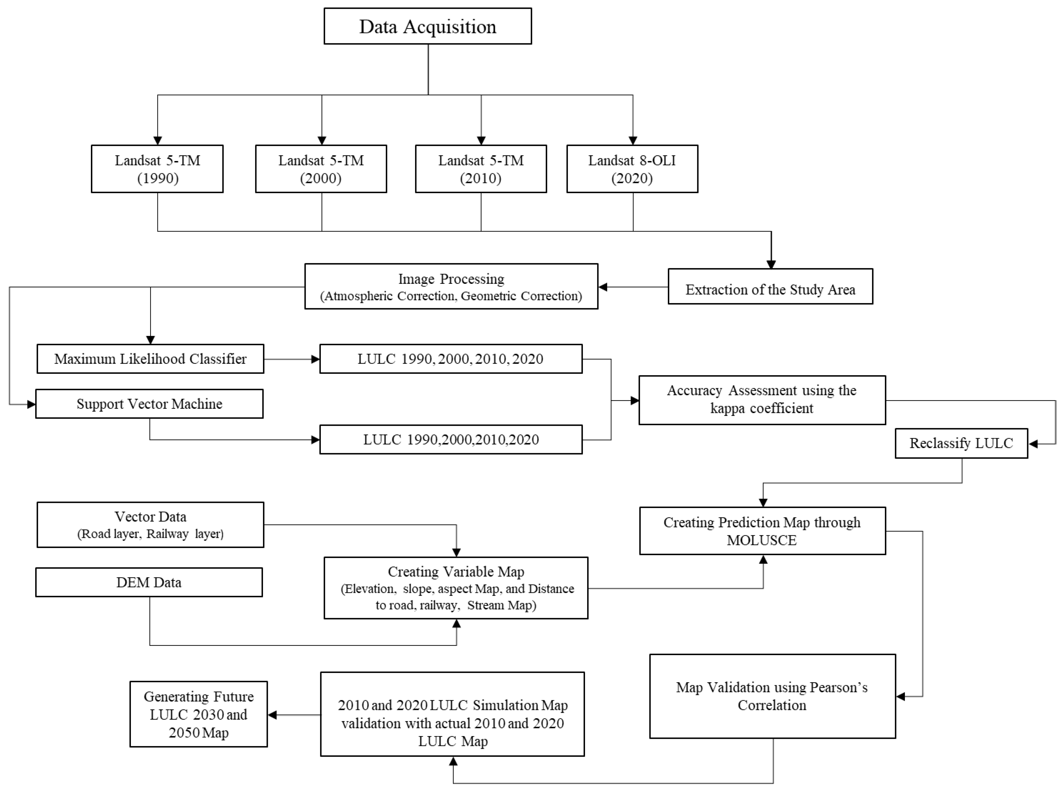
2. Materials and Methods

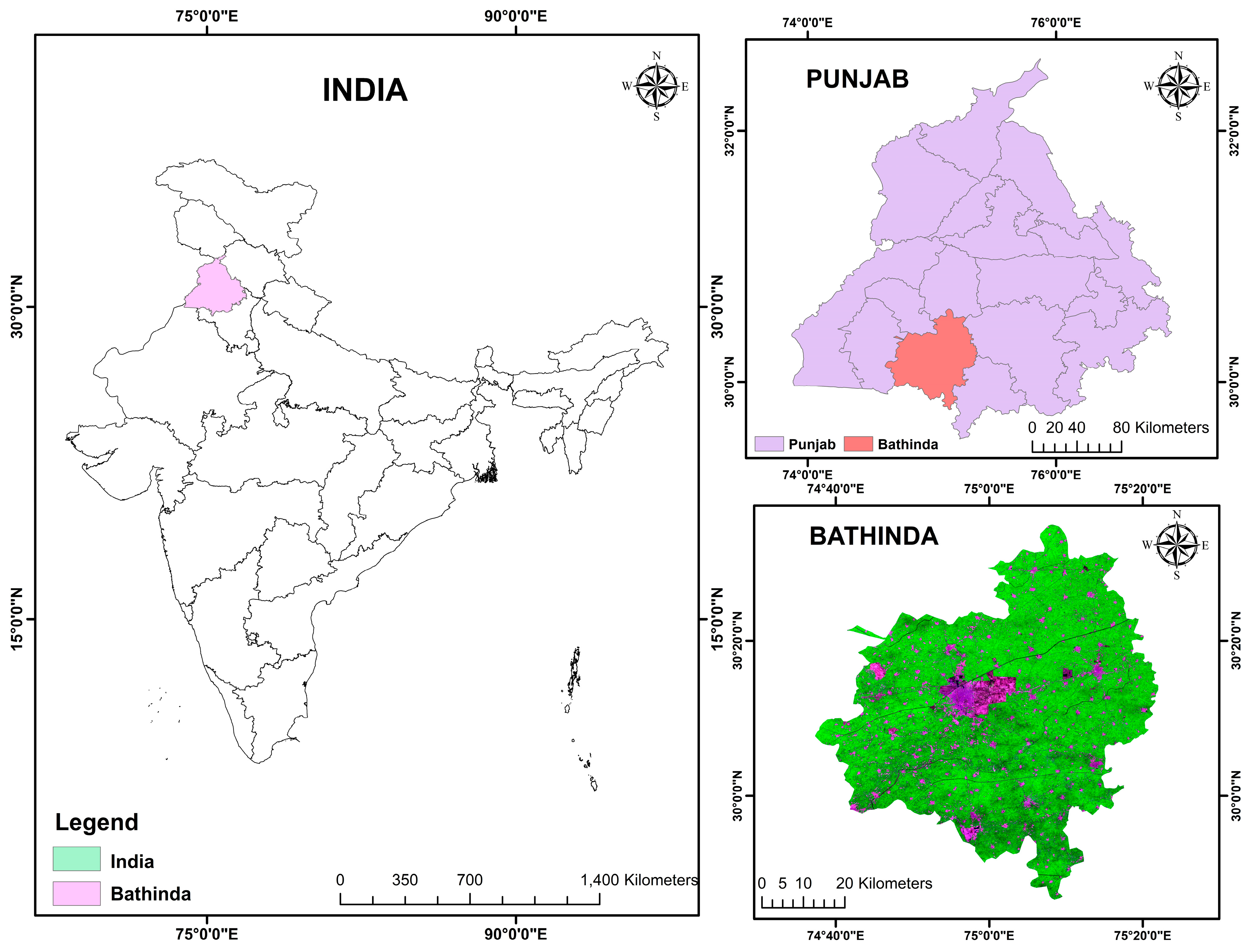
2.1. Study Area

Bathinda, also known as Bathinda, is one of the oldest cities in Punjab, located in the northern region of India (Figure 1). Spread across an area of approximately 3350 square kilometers, Bathinda district is geographically situated at 30.2000° N latitude and 74.9500° E longitude. The district is surrounded by Faridkot to the North, Muktsar to the West, Barnala and Mansa to the East, and the Sirsa district of Haryana state to the South. The district is named after its headquarters, Bathinda, one of Asia’s largest railway junctions. The district has a varied topography characterized by an alluvial plain with sandy soil. This area is predominantly flat, with a gradual slope from Northeast to Southwest, allowing the rivers in the region to flow in the same direction. The district of Bathinda is known for its rich agricultural productivity, thanks to the extensive irrigation facilities available, making it aptly referred to as the “Cotton Belt of India”. The primary crops grown here include cotton, rice, wheat, and vegetables. Several industries, including cotton ginning and pressing factories, thermal power plants, sugar mills, and fertilizer factories, complement the district’s agricultural productivity. Moreover, Bathinda is home to one of the biggest oil refineries in South Asia. The study focuses on the Bathinda District due to its rapid urbanization, yet alternative case study locations warrant consideration for broader insights. Feasible alternatives include Jaipur, Chittagong, and Lima, each offering unique urbanization challenges. Bathinda’s selection as a case study presents key advantages. Rich data availability on land cover changes and socio-economic factors bolsters the study’s empirical foundation. Diverse dynamics, encompassing industrialization, population growth, and agriculture, provide a multifaceted landscape for analysis. The study’s local relevance aligns with India’s urbanization concerns. Addressing issues like water resource management and urban-environmental balance is pertinent within the Bathinda context. While enhancing local relevance, the Bathinda case study’s findings may have limited generalizability due to region-specific complexities. Exploring alternative case study locations can provide a broader perspective on the efficacy and transferability of methodologies employed, especially the CA–Markov model. To bridge this gap, the study should outline the strengths and limitations of the Bathinda case study. Additionally, it should highlight the implications of this choice on research scope, findings, and utility in other regions. Discussing challenges and opportunities tied to alternative case study locations will underscore the approach’s alignment with broader objectives. This comprehensive approach ensures a well-rounded assessment of outcomes and their broader implications.

2.2. Data and Software Used

Four multi-temporal satellite data were used for modeling and prediction of the land use land cover. The satellite images of the years 1990, 2000, and 2010 of Landsat 5 Thematic Mapper (TM) and 2020 of Landsat 8 Operational Land Imager (OLI) [37] are downloaded from the United States Geological Survey (USGS) website.

Table 2. Details of the satellite data collected.

Satellite Data
Satellite Image	Sensor	Path/Row	Cloud Cover	Spatial Resolution	Acquisition Date
Landsat 5	TM	148/39	0.00	30 m	9 March 1990
Landsat 5	TM	148/39	0.00	30 m	17 February 2000
Landsat 5	TM	148/39	0.03	30 m	12 February 2010
Landsat 8	OLI-TIRS	148/39	0.26	30 m, Pan–15 m	24 February 2020

provides a comprehensive overview of the satellite data utilized in the context of this study. The data of SRTM DEM [38] is downloaded from the website of NASA Earth data with a spatial resolution of 30 m and was used to derive the Slope, Aspect, and Elevation map. All the software and packages used in the study are given in

Table 3. The software and packages used for specific needs and methodologies.

Software/Package	Purpose
ArcGIS 10.5	Geographic Information System (GIS) for spatial data analysis
QGIS 3.2	Geographic Information System (GIS) with Molusce plugin for CA Markov analysis
Google Earth Engine	A platform for geospatial data analysis and visualization
Remote Sensing Data	Utilized satellite imagery for land cover and change detection
Maximum Likelihood Classifier (MLC)	Employed for land cover classification
Support Vector Machine (SVM)	Used for land cover classification and analysis
Cellular Automaton–Markov Model	Framework for simulating and predicting land use changes
Multi-Criteria Decision-Making	Applied for land suitability analysis
Python	Calculating F1 Score and Significant Issue

.

The vector layers of Road and Railway are downloaded from the Diva GIS (https://www.diva-gis.org/ (accessed on 31 March 2022)) and OSM (https://www.openstreetmap.org/export (accessed on 11 September 2023)) websites. The layers of Distance to the road, distance to the railway, and distance to the stream are used as future prediction variable maps along with digital elevation data. All the variable maps are aligned geometrically for further prediction analysis. Due to their dynamic nature, these layers will probably incorporate uncertainties in predicting the area in future LULC scenarios. In the current study, the region is small; hence, the small uncertainties in the estimation are manageable when the study is on the management and sustainable development of the region. The dataset for variables taken in the current study is presented in

Table 4. Details of the secondary data collected.

Variables Map Data
	Data	Source	Map
1	Road Layer	Open Street Map	Distance to Road
2	Railway layer	Diva GIS	Distance to Railway
3	DEM ASTER	NASA Earth Data	Distance to Stream
4	DEM SRTM	NASA Earth Data	Slope Map
5	DEM SRTM	NASA Earth Data	Aspect Map
6	DEM SRTM	NASA Earth Data	Elevation Map

, and the methodology used for the future prediction study is shown in Figure 2.

2.3. Preprocessing of Data

Satellite data obtained from the USGS for 1990, 2000, 2010, and 2020 required pre-processing. Firstly, these images were geometrically corrected, ensuring each pixel was aligned correctly with its geographical position on the Earth’s surface. This step is important because any misalignment can cause errors in subsequent analyses. Then, the radiometric correction was performed on these images to adjust for sensor irregularities and atmospheric conditions. Each image was then resampled to a uniform spatial resolution of 30 m for consistency. The Shuttle Radar Topography Mission (SRTM) DEM data was downloaded from NASA Earth data (https://earthexplorer.usgs.gov/ (accessed on 11 September 2023)). It was first resampled to a uniform spatial resolution of 30 m to match the satellite data. Subsequently, the DEM was used to derive the slope, aspect, and elevation maps. These maps were then resampled and projected into the same coordinate system as the satellite images. The vector layers for road and railway networks were downloaded from Diva GIS and OSM. As these vector data sets can have varying levels of detail and may not be aligned with the raster datasets, a conversion was carried out. They were rasterized and resampled to the same spatial resolution (30 m) to match the satellite data. The distance to the road, the railway, and the stream layers were computed using these rasterized maps. After pre-processing each dataset, they were all integrated into a single GIS database. Each data layer was registered and georeferenced to the same coordinate system to ensure they aligned correctly. The final step in the pre-processing stage involved a thorough check to ensure that all the data layers were correctly aligned and that there were no missing data or anomalies. This step ensures the reliability and accuracy of subsequent analyses and model predictions.

2.4. Classification

In the present study, we performed two types of supervised classification to compare and check which one had high accuracy and choose the best one to perform the future prediction analysis. They are as follows.

2.4.1. Maximum Likelihood Classifier

The Maximum Likelihood Classifier is a popular approach for classifying images [30]. Based on the likelihood of their spectral values, it categorizes pixels or objects into several classifications. With the help of the Maximum Likelihood Classifier, we generated four different years of Land use land cover maps, 1990, 2000, 2010, and 2020, from the Landsat satellite data. It is a statistical technique that categorizes pixels or features according to the likelihood that each property belongs to a certain class. Using statistical models, the classifier calculates the likelihood that a pixel or feature belongs to each class. Given the class distribution parameters, it determines the probability of the observed attribute values. The pixel or feature being categorized is given the class with the highest probability. The properties of each class are presumed to follow a certain probability distribution, often a multivariate normal distribution, by the Maximum Likelihood Classifier. Maximum likelihood classification is implemented by calculating the following discriminant functions for each pixel in the image (Equation (1)):

g_i(x) = −1/2 ln|Σ_i| − 1/2 (x − μ_i)^T Σ_i⁻¹(x − μ_i) + lnP(C_i)

(1)

where, ln is the natural logarithm, |Σ_i| is the determinant of the covariance matrix Σ_i of class I, μ_i is the mean vector of class I, x is the feature vector of the pixel being classified, T denotes the transpose of a matrix or vector, Σ_i⁻¹ is the inverse of the covariance matrix Σ_i of class I, P(C_i) is the prior probability of class i

2.4.2. Support Vector Machine Classifier

Support vector machines (SVM) [39] is a powerful machine learning algorithm for classification and regression tasks. In my research work, we generated 1990, 2000, 2010, and 2020 LULC maps with the help of a Support Vector Machine Classifier and used them for future prediction Land use Land cover maps for 2030 and 2050. Because SVM offers effective handling of non-linear relationships between input features and land cover classes by using the kernel trick. This technique enables SVM to efficiently handle high-dimensional data by relying on support vectors, a subset of training samples. By incorporating class weights or cost-sensitive learning techniques, SVM can address imbalanced class distributions and prevent bias toward majority classes. SVM can be a good choice for LULC mapping; it is important to evaluate and compare its performance with other classifiers.

LULC mapping often involves high-dimensional data, such as remote sensing imagery. SVM efficiently handles such data by relying on support vectors, avoiding overfitting, and being computationally efficient. It can also handle imbalanced class distributions using class weights or cost-sensitive learning techniques.

2.5. Accuracy Assessment

In our study, we employed the Kappa coefficient [40] method to perform the accuracy assessment of both the supervised classification image techniques. The confusion matrix will have rows and columns representing the different land use classes. The overall accuracy is calculated by taking the sum of the correctly classified pixels (diagonal elements in the confusion matrix) and dividing it by the total number of sampled pixels. Producer’s accuracy and the user’s accuracy are also useful measures.

The formula for user accuracy is

User Accuracy = (Number of correctly classified samples for a specific class/Total number of samples classified as that class) × 100

The formula for producer accuracy is

Producer Accuracy = (Number of correctly classified samples for a specific class/Total number of ground truth samples of that class) × 100

The disparity between the actual agreement and the change agreement is often addressed using the Kappa coefficient to enhance the comprehension of the confusion matrix. Kappa’s coefficient is a more sophisticated measure of accuracy that considers the possibility of correctly classifying a pixel purely by chance. The Kappa coefficient was computed as (Equation (2)):

$$\tilde{\mathrm{k}}=\frac{\mathrm{N}\sum _{\mathrm{i}=1}^{\mathrm{r}}{\mathrm{X}}_{\mathrm{i}\mathrm{i}}\sum _{\mathrm{i}=\mathrm{i}}^{\mathrm{r}}({\mathrm{X}}_{\mathrm{i}+}\times {\mathrm{X}}_{+\mathrm{i}})}{{\mathrm{N}}^2-{\sum }_{\mathrm{i}=\mathrm{i}}^{\mathrm{r}}({\mathrm{X}}_{\mathrm{i}+}\times {\mathrm{X}}_{+\mathrm{i}})}$$

(2)

The formula given is for the Kappa coefficient, where ‘r’ represents the number of rows (or classes), ‘X_ii’ is the compute in the cell for its column and row, ‘X_i+’ is the overall of its row, ‘X_+i’ is the overall of its column, and ‘N’ is the whole number of pixels sampled.

At last, the F1-score was calculated, which is a balanced metric for evaluating classification models. It combines precision (correct positive predictions) and recall (capturing actual positives) into a single value. This is helpful when handling imbalanced data or when both false positives and false negatives matter. The F1-score is the harmonic mean of precision and recall, providing an overall measure of accuracy.

The F1-score is the harmonic mean of precision and recall, providing a balance between these two metrics. The distinctive features of the F1 score have been discussed in the literature [41,42]. It is calculated using the formula (Equation (3)):

F1 = 2 × Precision × Recall/Precision + Recall

(3)

The significant issue was calculated after the F1 Score. Significant issues in classification models refer to important problems affecting performance. They include low accuracy, imbalanced classes (leading to biased predictions), misclassification of specific classes, poor sensitivity or specificity, performance changes over time, and domain-specific concerns. Addressing these issues involves refining models, improving features, adjusting hyperparameters, and ensuring data quality to enhance predictive reliability.

2.6. CA–Markov Model for Land Use Change Prediction

This study adopted the CA–Markov model with the MOLUSCE module embedded in the QGIS software version 2.8.3. The integration of MOLUSCE further enhanced the model’s predictive capabilities by incorporating multiple criteria for evaluating the suitability of different LULC types. Once the data are collected, the CA–Markov model is calibrated and validated using historical land use data for a specific period. The historical land use data are used to estimate the transition probabilities between different land use categories. The model is adjusted to match the observed land use changes during calibration. This calibration process ensures that the model accurately captures the historical land use dynamics in the Bathinda District.

The simulated land use patterns are compared to the observed land use patterns for a different period to validate the model. This validation step assesses the accuracy and reliability of the CA–Markov model in predicting land use changes. If the model produces satisfactory results during the validation phase, it can be considered a reliable tool for projecting future land use patterns. Once the CA–Markov model is calibrated and validated, it can be used to simulate future land use scenarios in the Bathinda District. The model projects how land use categories will likely change over time by considering the historical land use dynamics. The simulation provides insights into the potential impacts of different land use scenarios on the district’s sustainability, allowing decision-makers to evaluate the consequences of alternative land use policies and interventions.

3. Results

3.1. Predicting the Best Classifier

For all four years, 1990, 2000, 2010, and 2020, confusion matrices of the signatures acquired from supervised classification training using ML (

Table 5. The classification accuracy for ML classifier on all years of LULC.

Reference Data
	1990 LULC		2000 LULC		2010 LULC		2020 LULC
LULC Classes	User Accuracy (%)	Producer Accuracy (%)	User Accuracy (%)	Producer Accuracy (%)	User Accuracy (%)	Producer Accuracy (%)	User Accuracy (%)	Producer Accuracy (%)
Barren land	80	80	70	78	70	63	80	80
Vegetation, class	60	60	60	50	70	78	60	67
Agriculture	83	83	86	82	76	88	84	75
Waterbody	60	100	80	89	90	90	100	100
Wetland	60	75	40	100	40	100	90	100
build-up area	90	65	80	100	70	39	80	100
Fallow land	77	67	80	50	70	54	80	73
Kappa index	0.69		0.68		0.64		0.78
Overall Accuracy	75.5%		75.2%		71%		82.3%

) and SVM (

Table 6. Accuracy assessement for SVM classifier.

Reference Data
	1990 LULC		2000 LULC		2010 LULC		2020 LULC
LULC Classes	User Accuracy (%)	Producer Accuracy (%)	User Accuracy (%)	Producer Accuracy (%)	User Accuracy (%)	Producer Accuracy (%)	User Accuracy (%)	Producer Accuracy (%)
Vegetation	80	89	90	100	90	100	100	83
Agriculture	90	100	100	100	100	83	90	100
Waterbody	92	81	92	92	92	96	95	95
Wetland	80	100	90	100	100	100	100	100
build-up area	100	100	90	100	70	100	90	90
Fallow land	80	100	80	73	90	75	70	100
Kappa	90	75	90	75	90	82	100	83
index	0.85		0.88		0.88		0.91
Overall	88.5%		91%		91%		93%

) classifier table are shown below.

In

Table 7. F1 scores for two cases, along with the class labels and meanings, followed by predictions of significant issues based on the F1 scores.

Class Label	F1 Score (MLC)	F1 Score (SVM)	Significant Issue (MLC)	Significant Issue (MLC)
Barren land	0.8000	0.9071	No	No
Vegetation	0.6331	0.9474	Yes	No
Agriculture	0.7925	0.9500	No	No
Waterbody	1.0000	1.0000	No	No
Wetland	0.9474	0.9000	No	No
Build-up area	0.8889	0.8235	No	No
Fallow land	0.7634	0.9071	No	No

, “Significant Issue” indicates whether a class has a significant issue based on its F1 score. Here are the predictions. In MLC, significant issues are predicted for Class 2 (Vegetation) due to its low F1 score, indicating potential misclassification issues. In SVM, no significant issues are predicted for any class based on the F1 scores, as all F1 scores are relatively high. The significance of an issue depends on the application context and the specific goals of your classification model.

The result maps of the land use of both classifiers are validated by generating the standard random sampling points and are crosschecked by using Google Earth Pro. Then, the accuracy is recorded for all the classes in the tabular form (confusion matrix) for every year. The accuracy is calculated as how much accuracy is available in each class and each year map. The results are noted in tabular form. After analyzing the accuracy of the images of both classifiers, we concluded that the maps generated using the support vector classifiers (OA = 82.3%) have more accuracy than those generated using Maximum Likelihood Classifiers (OA = 93%).

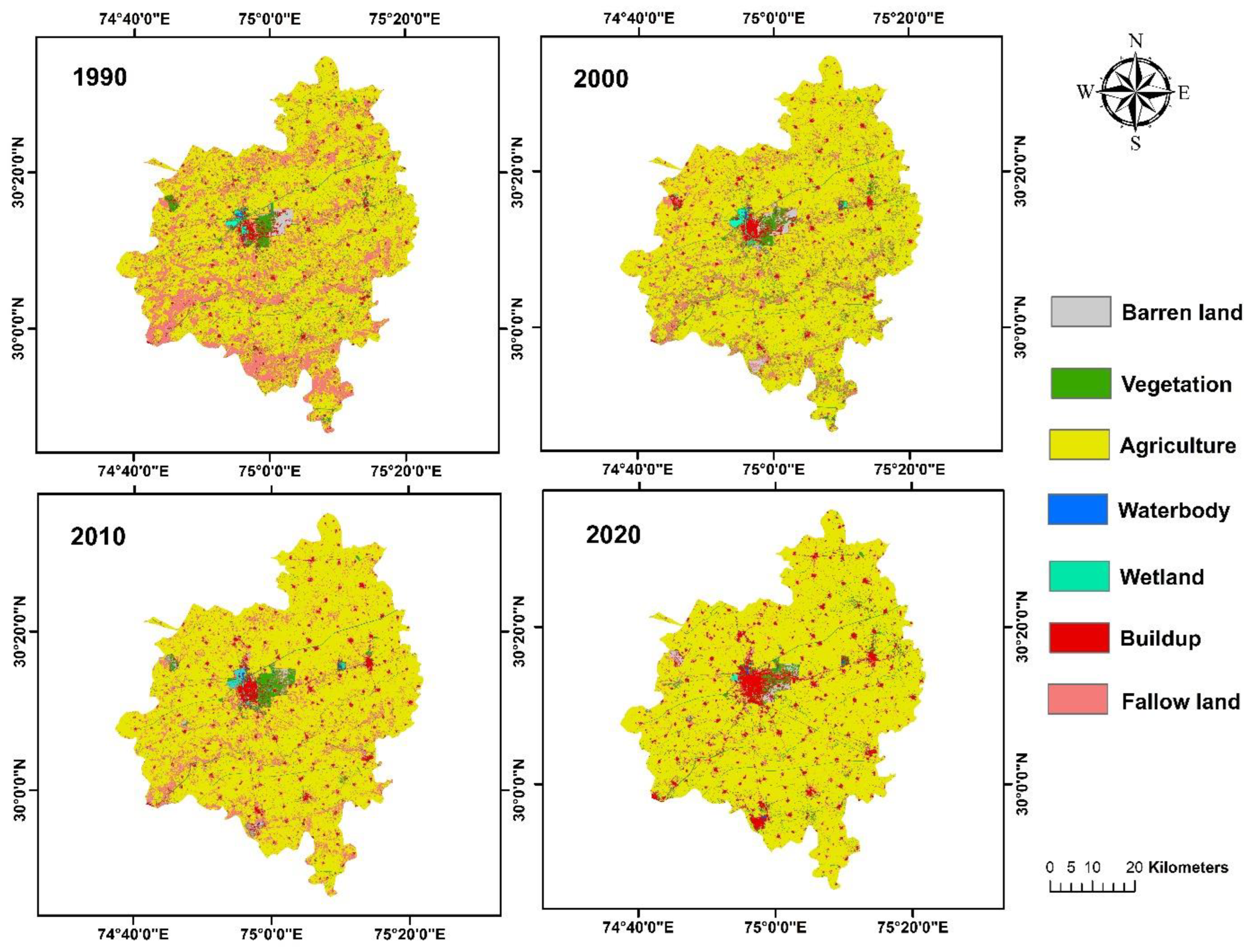
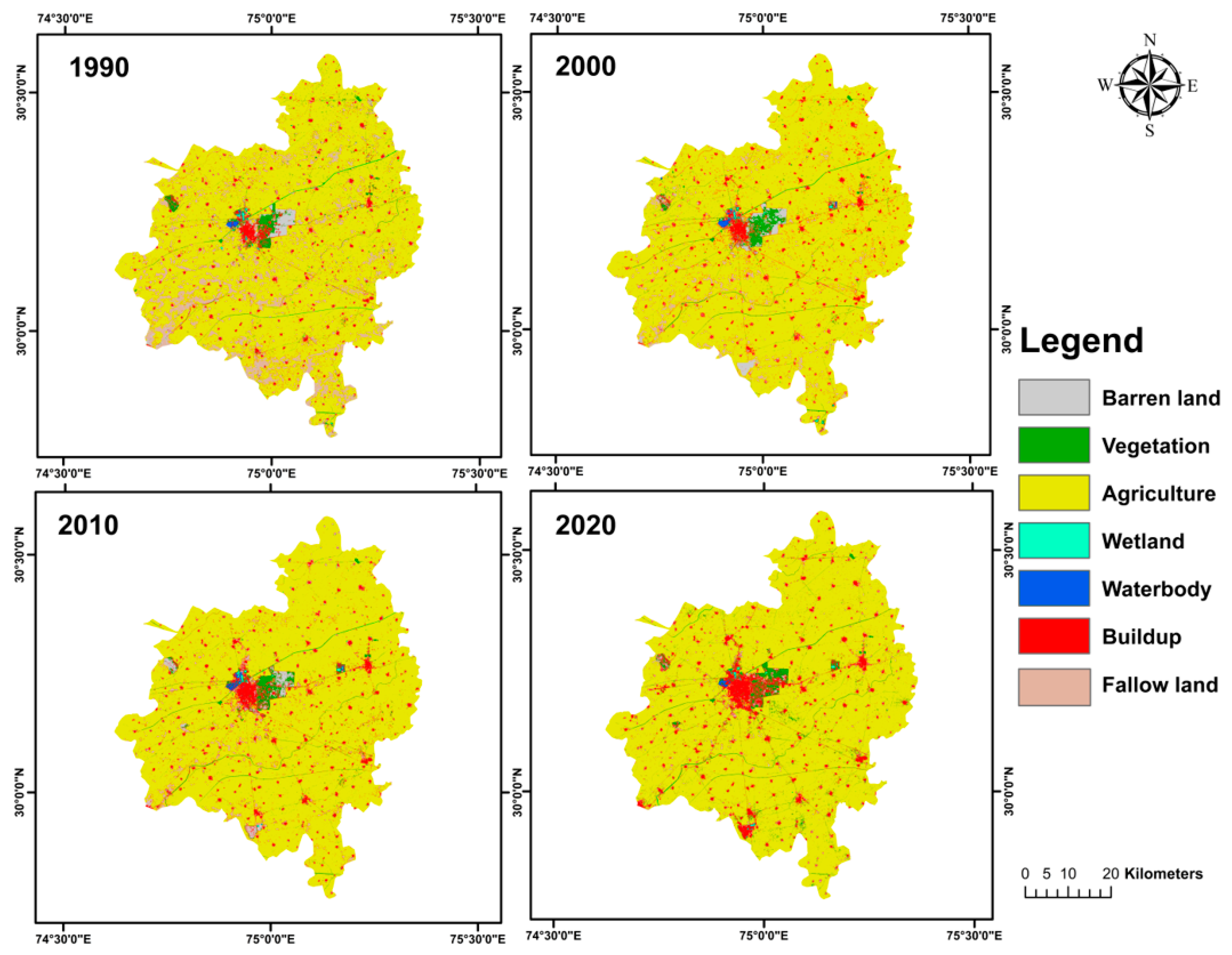
3.2. Land Use and Land Cover Change 1990–2020

The land uses land cover generated by supervised classification using the support vector machine classifier and prepared land use land cover maps of the years 1990, 2000, 2010, and 2020 (Figure 3). The most striking observation is the continuous decrease of barren and fallow land over the years (

Table 8. The area and percentage-wise classification of LULC using SVM from 1990 to 2020.

Changes LULC 1990 to 2020
Classs Name	LULC 1990 Area		LULC 2000 Area		LULC 2010 Area		LULC 2020 Area
	Km2	%	Km2	%	Km2	%	Km2	%
Barren land	55.2	1.63	45	1.32	32.5	0.96	17.7	0.52
Vegetation	81.3	2.40	91.4	2.7	93	2.7	123.2	3.6
Agriculture	2597.4	76.7	2872.1	84.8	2886.6	85.2	2859.6	84.4
Waterbody	13.4	0.39	11.4	0.33	9.8	0.28	8.1	0.23
Wetland	2.9	0.08	5.2	0.15	5	0.14	2.3	0.06
Build up	136.4	4.0	155.8	4.6	170.3	5	203.2	6.0
Fallow land	498.2	14.7	204	6.0	187.6	5.5	171	5

). Barren land has declined from 1.63% in 1990 to 0.52% in 2020, while fallow land has seen a more substantial decrease, from 14.7% in 1990 to 5% in 2020. This may suggest effective land use planning and management or increased human activity and development (

Table A1. LULC areas of all four years of MLC classification images.

Area of MLC Classified LULC Classes
		1990 LULC		2000 LULC		2010 LULC		2020 LULC
	Classes	Area sq km	Area (%)	Area sq km	Area (%)	Area sq km	Area (%)	Area sq km	Area (%)
1	Barren land	29.5	0.87%	27.5	0.81%	19.4	0.57%	21.7	0.64%
2	Vegetation	215.3	6.30%	276.1	8.10%	178	5.25%	168.7	4.90%
3	Agriculture	2115.7	62%	2477.6	73.10%	2587	76.40%	2783.4	82.20%
4	Waterbody	7.4	0.21%	6.1	0.18%	7.6	0.22%	6.3	0.18%
5	Wetland	10.7	0.31%	17.7	0.55%	19.2	0.56%	19.1	0.58%
6	Build up	107	3.10%	114.9	3.30%	122.4	3.60%	224.8	6.60%
7	Fallow land	899.4	26.50%	464.5	13.70%	451.7	13.30%	161	4.70%

, Figure A1).

Simultaneously, built-up land has consistently increased over the same period, rising from 4% in 1990 to 6% in 2020. This could reflect population growth, urbanization, and industrial development, which often demand expanded built-up areas. Interestingly, the percentage of agricultural land initially increased from 76.7% in 1990 to 85.2% in 2010 but slightly decreased to 84.4% by 2020.

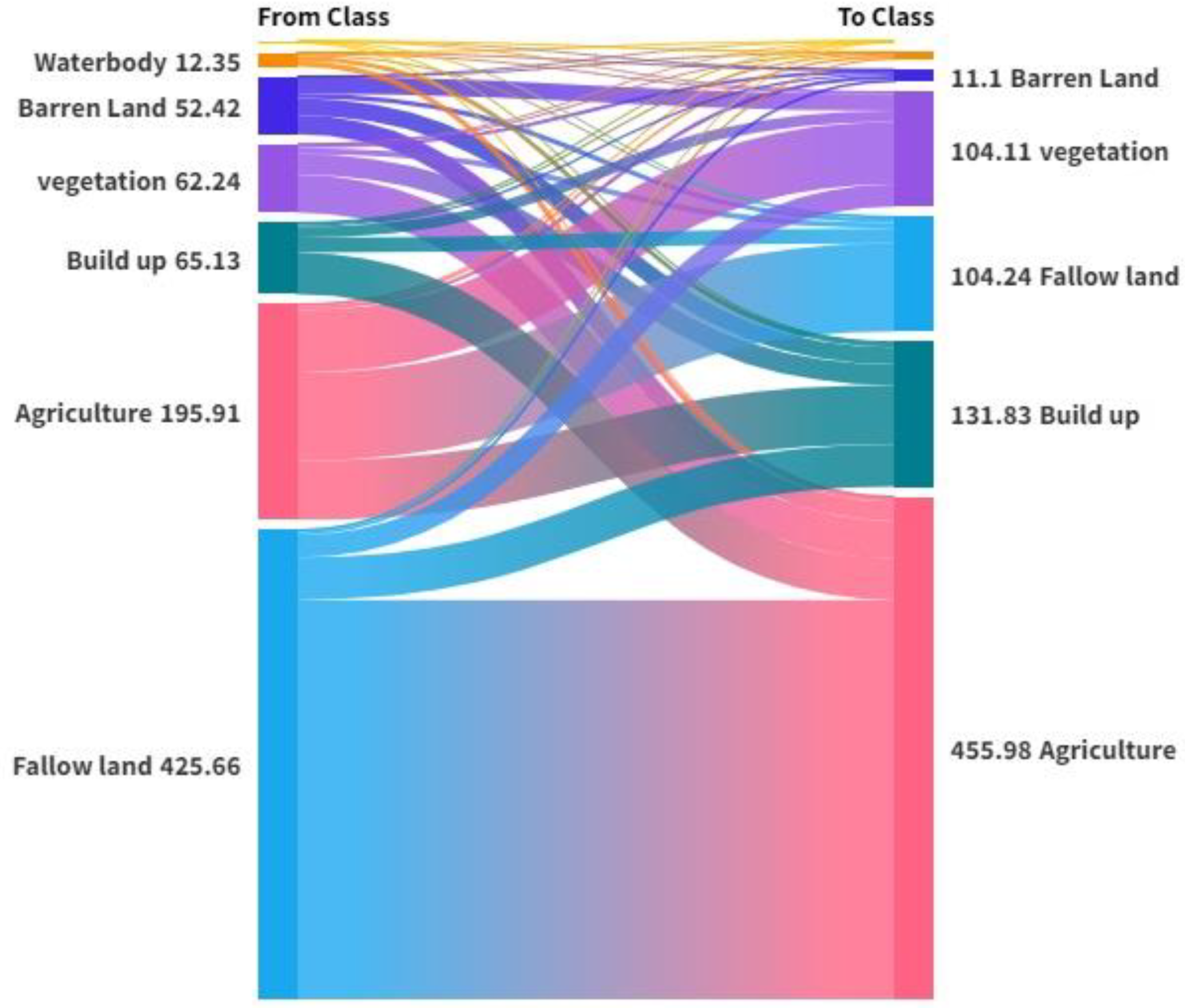
3.3. Land Use Transformation

Figure 4 represents land use and land cover (LULC) transformations from 1990 to 2020. It shows how different land classes have transformed into one another during this time period. Let us discuss the key findings and implications of these transformations:

3.3.1. Barren Land to Other Classes

Barren land has transformed into various land classes, including vegetation, agriculture, water bodies, wetlands, and built-up areas. The most significant transformation is from barren land to agriculture, with 18,864 pixels (16.98 sq km) transformed, indicating an expansion of agricultural activities. Transformation into built-up areas is also substantial, with 17,159 pixels (15.44 sq km) converted. This signifies urbanization and infrastructure development. Transformation into fallow land (4743 pixels, 4.27 sq km) may suggest unused land or undergoing recovery.

3.3.2. Vegetation to Other Classes

Vegetation has transformed into multiple classes, the most prominent being agriculture (38,026 pixels, 34.22 sq km) and built-up areas (21,048 pixels, 18.94 sq km). These transformations indicate the conversion of natural vegetation into agricultural land and urban areas, potentially driven by population growth and economic activities.

3.3.3. Agriculture to Other Classes

Agriculture has transformed into various categories, substantially converting into built-up areas (59,574 pixels, 53.62 sq km). This transformation highlights urban expansion and the conversion of agricultural land for non-agricultural purposes.

3.3.4. Waterbody to Other Classes

Water bodies have transformed into built-up areas (4594 pixels, 4.13 sq km) and agriculture (5570 pixels, 5.01 sq km), indicating land reclamation and infrastructure development.

3.3.5. Wetland to Other Classes

Wetlands have transformed, especially into built-up areas (1386 pixels, 1.25 sq km), which may raise concerns about ecological preservation and potential environmental impacts.

3.3.6. Build Up to Other Classes

Built-up areas have transformed into agriculture (41,808 pixels, 37.63 sq km) and vegetation (11,176 pixels, 10.06 sq km), signifying urban sprawl and potential agricultural abandonment in urban areas.

3.3.7. Fallow Land to Other Classes

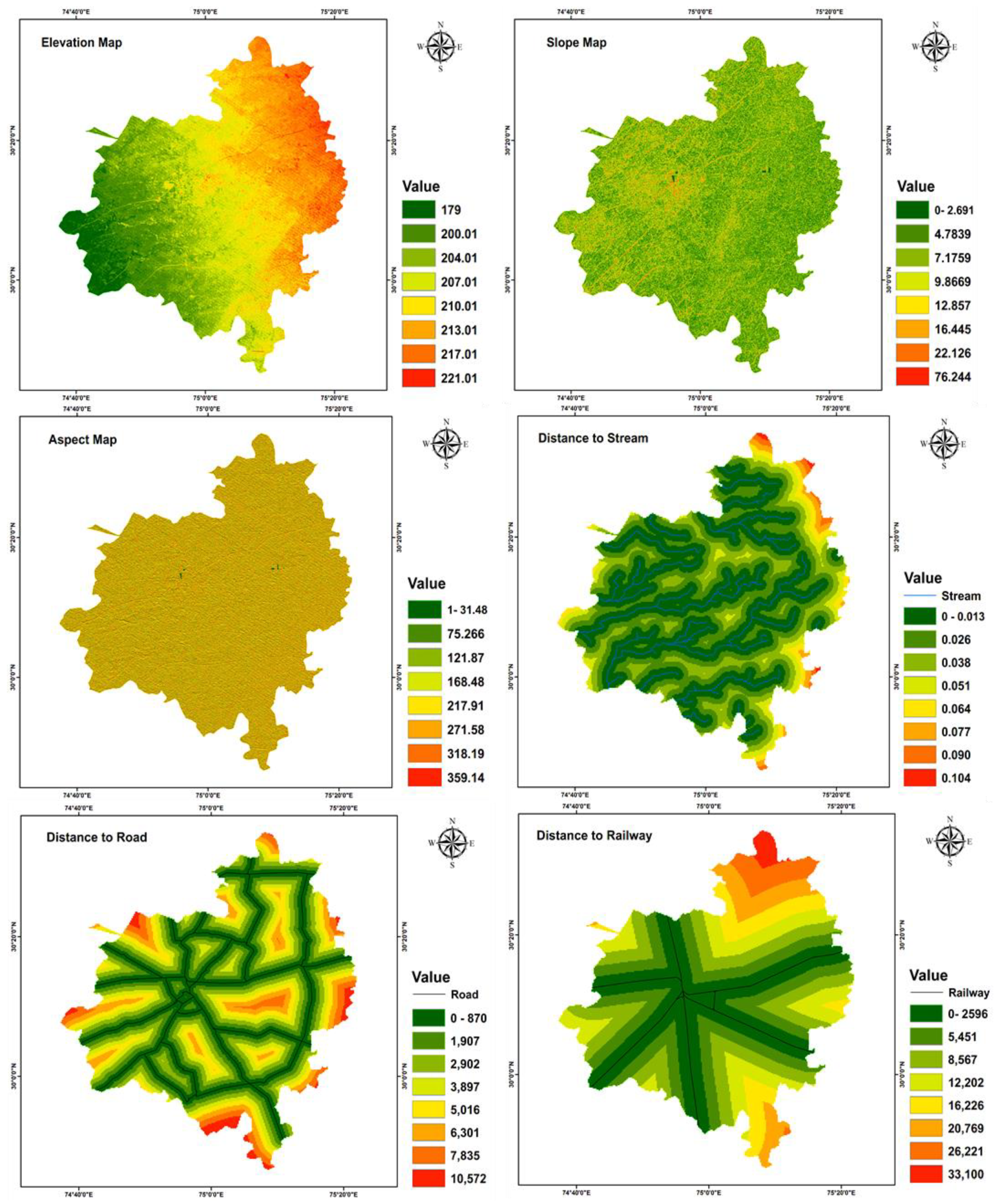
Fallow land has seen a significant transformation into agriculture (402,350 pixels, 362.12 sq km), suggesting intensive agricultural activities or reclamation of previously unused land.

3.4. Variables Map

In the current study, we used variable maps (Figure 5), which help us predict future land use land cover changes and can work as the driving factors. Using variable maps such as distance to road, distance to stream, distance to railway, elevation, aspect, and slope is a common approach in land use land cover (LULC) future prediction studies. These variables provide valuable information about the landscape’s topographic and transportation characteristics, which can influence land cover changes. Its results herein are unnecessary as it is a part of the work used for the current study.

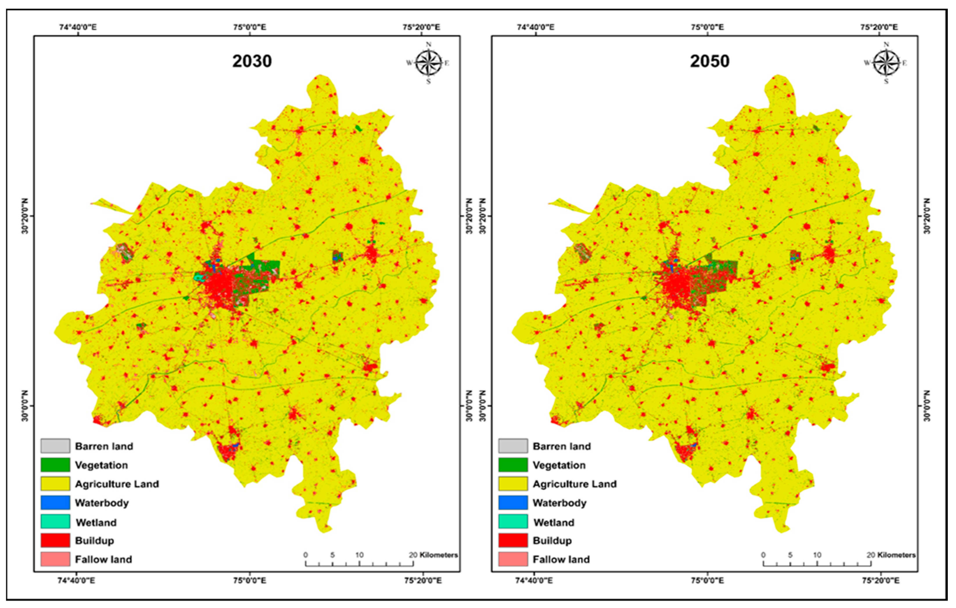
3.5. Predicting of Future LULC

In the present study of land use land cover future prediction, we generated the land use land cover for 2030 and 2050 (Figure 6) using the CA–Markov model. The land uses land cover generated by supervised classification using the support vector machine classifier and prepared land use land cover maps of the years 1990, 2000, 2010, and 2020. The LULC maps of 2010 and 2020 are used to generate the land use prediction map for 2030, and the maps of 1990 and 2020 are used to generate the land use prediction map for the year 2050.

We can observe the predicted LULC classes and the changes in land use patterns over the years in the future (

Table 9. Area and percentage of predicted LULC 2030 and 2050.

LULC Classes		LULC 2030 Predicted Area		LULC 2050 Predicted Area
		Km2	%	Km2	%
1	Barren land	15.8	0.46	11.3	0.33
2	Vegetation	132.2	3.90	158.5	4.6
3	Agriculture	2870.3	84.7	2898.4	85.6
4	Waterbody	7.7	0.22	5.6	0.16
5	Wetland	2.1	0.06	0.68	0.02
6	Build up	215.5	6.56	235.3	6.95
7	Fallow land	141	4.1	74.3	2.19

). In the predicted map of 2030, we can observe that agriculture is going to cover over 84.7% of the Bathinda district, covering 2870.3 km², and with a built-up area of over 6.56% of the district covering 215.5 km² remaining, all the land use classes, such as barren land, vegetation, waterbody, wetland, and fallow land are occupies a small area of 0.46 percent with 15.8 km², 3.90 percent with 132.2 km², 0.22 percent with 7.7 km², 0.06 percent with 2.1 km², 4.1 percent with 141 km² respectively. We can notice from Table 9 that the agriculture and build-up area will increase from the year 2020, and the rest of the land use patterns will decrease to a greater extent.

In the predicted map of the year 2050 (Figure 6), we can observe that agriculture is going to cover over 85.6 percent of the Bathinda district, covering 2898.4 km², and with the built-up area of over 6.95 percent of the district covering 235.3 remaining all the land use classes such as barren land, vegetation, waterbody, wetland, and fallow land are occupies a small area of 0.33 percent with 11.3 km², 4.6 percent with 158.5 km², 0.16 percent with 5.6 km², 0.02 percent with 0.68 km², 2.19 percent with 74.3 km², respectively. We can notice from Table 9 that the area of agriculture, build-up area, and vegetation is going to increase from the year 2030, and the rest of the land use patterns are going to decrease to a greater extent.

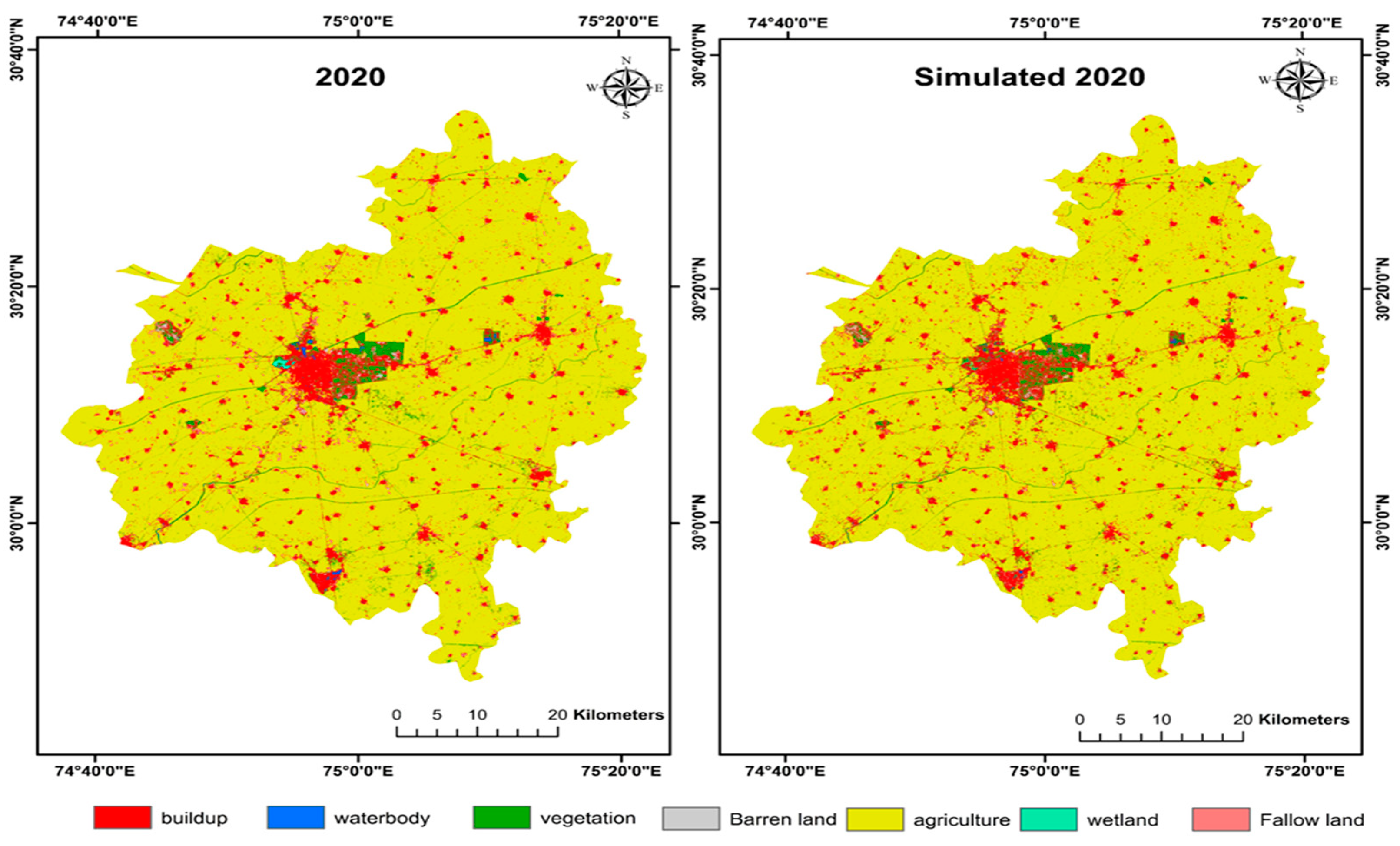
3.6. Model Validation

CA–Markov model was validated by comparing the observed and simulated LULC maps for 2020 (Figure 7), resulting in derived K_no, K_standard, Kl_ocation, and K_quantity values. Moreover, the kappa variations K_no (0.97), K_standard (0.95), and K_location (0.97) in this study indicated a satisfactory level of accuracy.

4. Discussion

Land use and land cover (LULC) changes are important indicators of a region’s environmental and socioeconomic transformations. Bathinda, one of the fastest-growing cities in Punjab and India, has experienced significant LULC changes in the past three decades due to rapid urbanization and industrialization. Rathore et al. (2019) [43] published a report on India’s future scenario of industrialization and urbanization and its impact on environmental sustainability. This report shows that trends in India’s energy sector underscore the significance of urbanization and industrialization as key drivers. While the COVID-19 pandemic has introduced uncertainties, these drivers remain pivotal. The urban population is projected to grow by 270 million by 2040, necessitating substantial infrastructure development and energy-intensive building materials. This expansion prompts increased demand for steel and cement, reflecting the energy requirements of construction. Urbanization also prompts a shift in household energy use towards electricity due to rising appliance ownership and air conditioning demand. However, despite policy initiatives, transportation demand, driven by urbanization, leads to congestion and increased oil consumption.

For the change of land use landcover pattern of the region, The transportation such as railways and roadway networks plays a major role as the expansion of the cities and major settlements are more focused in the areas with good transport feasibility as it supports for the growth and development of cities and movement of the goods and services, besides the drainage facilities such as the canals and rivers also have their role in determining the land use pattern as from the ancient times settlements are mostly established near the rivers and water available regions as the agriculture also depended on water availability of the region, the slope, elevation and aspect factors have their weightage as the areas highly elevated from ground level tend to have low population and the areas with slopes cannot have much infrastructure and development as compared to the plain regions, the soil type parameter have no much effect on the urban growth or the land use change as soil type or fertile soil can only enhance the agriculture production but not a growth factor for the urban expansion or development. Other than these, all the remaining parameters directly or indirectly depend on or are based on these main parameters only.

Our study finds similar dynamics in land use changes within the Bathinda District. The results of this study showed that the urban area increased from 13.4 km² in 1990 to 96.8 km² in 2050, indicating a high demand for land for residential, commercial, and industrial purposes. The rapid urbanization and industrialization observed in India resonate with our study’s increased built-up land and industrial expansion. The surge in energy demand from urbanization and industrial growth aligns with our findings of shifts in land use patterns requiring careful energy management strategies. Similarly, our study emphasizes the role of informed decision-making and policy implementations for sustainable land use planning. This finding is consistent with the general trend of urbanization in India, which is driven by factors such as population growth, economic development, migration, infrastructure, and policy [44]. Urbanization can have positive impacts, such as improved income, employment, education, health care, and infrastructure, but also negative impacts, such as loss of agricultural land, depletion of water resources, pollution of air, water, and soil, degradation of biodiversity, generation of waste, congestion of traffic, and inequality of income and access [45]. The results also showed that the barren land decreased from 55.2 km² in 1990 to 5.6 km² in 2050, implying better land management or increasing human activity. Barren land is usually unproductive and prone to soil erosion and desertification. Reducing barren land can enhance soil quality and fertility, increase water retention and infiltration, and prevent land degradation. Converting barren land to other LULC classes may also have trade-offs, such as loss of natural habitats, alteration of hydrological cycles, and emission of greenhouse gases. The statement above draws on some general knowledge about the characteristics and impacts of barren land, which can be found in various sources such as [46,47].

The results showed that the vegetation area increased from 81.3 km² in 1990 to 205.6 km² in 2050, reflecting a balance between urbanization and ecological conservation. Vegetation includes forests, grasslands, shrubs, and wetlands that provide various ecosystem services such as carbon sequestration, oxygen production, climate regulation, biodiversity conservation, soil protection, water purification, flood control, recreation, and tourism. Increasing vegetation areas can enhance the environmental quality and resilience of Bathinda. However, vegetation may also face threats from urban expansion, agricultural intensification, climate change, invasive species, fire, and pests. The finding is consistent with the general pattern of vegetation recovery in India, which is driven by various factors such as afforestation programs, land use policies, rural-urban migration, agricultural modernization, and market forces. Vegetation recovery can have positive impacts such as mitigating climate change, enhancing biodiversity, improving soil health, reducing water stress, and providing livelihood opportunities. Vegetation recovery can also have trade-offs, such as displacing local communities, increasing human-wildlife conflicts, altering hydrological cycles, and introducing exotic species.

The finding has important implications for the sustainable development and management of land resources in Bathinda and its surroundings. On the one hand, increasing vegetation area can contribute to the achievement of several Sustainable Development Goals (SDGs), such as SDG 13 (Climate Action), SDG 15 (Life on Land), and SDG 17 (Partnerships for the Goals). On the other hand, increasing vegetation area can also pose challenges for the implementation of other SDGs such as SDG 1 (No Poverty), SDG 2 (Zero Hunger), and SDG 11 (Sustainable Cities and Communities). Therefore, there is a need for integrated and adaptive approaches that can balance the multiple objectives and interests of different stakeholders in land use and land cover changes in Bathinda. The results finally showed that the agriculture area increased from 2597.4 km² in 1990 to 2859.6 km² in 2020, then stabilized at 2898.4 km² in 2050. Agriculture is the main livelihood source for most of Bathinda’s rural population. It contributes to food security, income generation, and employment opportunities. Increasing agriculture areas can meet the growing demand for food and other agricultural products due to population growth and urbanization. However, agriculture may also have negative impacts on the environment, such as loss of natural habitats, depletion of water resources, pollution of air, water, and soil, degradation of biodiversity, generation of waste, and emission of greenhouse gases.

The finding is consistent with the general trend of agricultural expansion in India, which is driven by factors such as population growth, economic development, food security, poverty alleviation, and policy support [48]. Agriculture accounts for about 17.5% of India’s GDP and employs about 41.49% of its workforce [49]. India ranks second in the world in terms of net cropped area and first in gross cropped area 5. India is also one of the leading producers and consumers of various agricultural commodities such as cereals, pulses, oilseeds, fruits, vegetables, milk, eggs, meat, and fish. Increasing agriculture areas can enhance the productivity and profitability of farming and improve the population’s food security and nutrition status. Agriculture may also have trade-offs with the environment and sustainability. Agriculture is one of the major consumers of water resources in India, accounting for about 80% of the total water use. Agriculture is also one of the major sources of water pollution due to the use of fertilizers, pesticides, and animal wastes. Agriculture is also one of the major contributors to greenhouse gas emissions in India, accounting for about 18% of the total emissions. Agriculture is also one of the major causes of land degradation in India, affecting about 120 million hectares or 36% of the total land area. Agriculture is also one of the major drivers of biodiversity loss in India, leading to habitat fragmentation, invasion of alien species, overexploitation of resources, and genetic erosion.

The study found that the water landscapes, which include rivers, canals, ponds, lakes, and reservoirs, are expected to shrink from 13.4 km² in 1990 to 5.6 km² in 2050, providing possible issues for water resources. The study also found that the wetlands, which are a subset of water landscapes that support aquatic vegetation and wildlife, are predicted to decline from 3.4 km² in 1990 to 1.6 km² in 2050. The finding is consistent with the general trend of water scarcity and degradation in India, driven by various factors such as population growth, urbanization, industrialization, agriculture, climate change, and pollution [50]. Water is vital for human health, food security, energy production, and ecosystem services. India has about 4% of the world’s freshwater resources but supports about 18% of the world’s population [50]. India’s per capita water availability has declined from 1816 cubic meters in 2001 to 1545 cubic meters in 2011 and is projected to further decline to 1140 cubic meters by 2050. India’s water quality is also deteriorating due to untreated domestic and industrial effluents, agricultural runoff, and solid waste being discharged into the water bodies [51]. The finding has important implications for the sustainable development and management of water resources and wetlands in Bathinda and its surroundings. On one hand, shrinking water landscapes and wetlands can pose challenges for meeting the growing demand for water for various purposes such as drinking, irrigation, industry, and recreation. Shrinking water landscapes and wetlands can also affect the hydrological cycle, groundwater recharge, flood control, soil erosion, climate regulation, biodiversity conservation, and cultural values. On the other hand, shrinking water landscapes and wetlands can also provide opportunities for improving the efficiency and equity of water use and allocation, enhancing the quality and quantity of water resources, restoring and protecting the ecological functions and services of water landscapes and wetlands, and promoting integrated water resources management.

Therefore, there is a need for sustainable management of agriculture area changes in Bathinda and its surroundings. On the one hand, increasing the agriculture area can support the livelihoods and well-being of millions of farmers and consumers in Bathinda. On the other hand, increasing agricultural area can also pose challenges for the conservation and restoration of natural resources and ecosystems in Bathinda. Some of the possible measures that can be taken are adopting climate-smart agriculture practices that can enhance productivity, adaptation, and mitigation; promoting organic farming and integrated pest management that can reduce chemical inputs and pollution; improving irrigation efficiency and water harvesting that can save water and prevent salinization; implementing soil health cards and nutrient management that can improve soil quality and fertility; diversifying crops and livestock that can increase income and resilience; enhancing agroforestry and agro-biodiversity that can provide multiple benefits; strengthening farmer producer organizations and cooperatives that can improve market access and bargaining power; and monitoring and evaluating the agriculture area changes using remote sensing and GIS tools. The finding has important implications for Bathinda’s environmental and social aspects and surroundings. On one hand, urbanization and industrialization can bring positive benefits such as increased income, employment, education, health care, and infrastructure. On the other hand, urbanization and industrialization can also pose challenges such as loss of agricultural land, depletion of water resources, pollution of air, water, and soil, degradation of biodiversity, generation of waste, congestion of traffic, and inequality of income and access. Therefore, there is a need for proper planning and management of land use and land cover changes in Bathinda, considering the trade-offs between economic growth and environmental sustainability.

The decrease in barren and fallow land over the years is a significant observation. These changes may indicate effective land use planning and management or increased human activity and development. Previous studies have highlighted the importance of land management practices and interventions in reducing barren land and promoting sustainable land use [52]. The increase in built-up land over the same period is noteworthy. This upward trend reflects population growth, urbanization, and industrial development, often driving the expansion of built-up areas. Numerous studies have documented the impact of urbanization on land use change and the transformation of agricultural or natural land into built-up areas [53]. The growth of built-up land emphasizes the need for careful land use planning to ensure sustainable urban development and minimize the adverse effects on the environment and natural resources. The percentage of agricultural land initially increased from 76.7% in 1990 to 85.2% in 2010 but slightly decreased to 84.4% by 2020. This fluctuation could be attributed to various factors, including changes in agricultural practices, land conversion, and urbanization. The transformation of agricultural land into built-up areas is a common phenomenon driven by urban expansion and infrastructure development [54]. However, it is crucial to balance urban growth and agricultural land preservation to ensure food security and sustainable rural development [55]. By utilizing tools such as the support vector machine classifier and generating land use land cover maps, researchers and planners can monitor land use dynamics, identify areas of concern, and inform policy interventions for sustainable land management [56].

Using variable maps in land use and land cover prediction allows researchers to capture the spatial heterogeneity and diverse factors influencing land cover changes. By considering variables such as distance to road, stream, and railway and terrain characteristics like elevation, aspect, and slope, the model can better simulate the spatial patterns of land use transitions and identify areas more prone to change. These variables provide valuable information about the landscape’s physical and infrastructural characteristics, which can guide land use planning and management strategies [57,58]. The variables taken here are based on previous studies on this in other areas.

Future forecasts help identify the dominant land use classes and their changing patterns over time. In the case of the Bathinda district, knowing that agriculture is predicted to cover a significant portion of the land in 2030 provides important information for planners to address the associated challenges and opportunities. It allows them to assess the impact on agricultural practices, water resources, and other aspects of land management. The forecast for 2030 indicates an increase in built-up areas, which can help guide infrastructure planning and development. It enables planners to identify suitable locations for residential, commercial, and industrial zones, considering transportation networks, utilities, and environmental considerations. Sustainable infrastructure development can promote efficient land use, reduce environmental impacts, and enhance the quality of life. With agriculture covering a significant portion of the land, sustainable land use planning should consider the need for a balance between agricultural and non-agricultural land uses. This may involve identifying areas suitable for urban expansion, green spaces, conservation areas, and infrastructure development while preserving fertile agricultural land. Future forecasts can highlight potential vulnerabilities and risks associated with land use changes. Planners can use this information to develop strategies for climate change adaptation, disaster risk reduction, and resilience-building measures. The forecasted 2050 increase in agricultural land and built-up areas indicates the direction of future land use changes. By recognizing these trends in advance, policymakers and planners can proactively address the associated challenges, such as urbanization pressures, agricultural intensification, and the need for infrastructure development.

With agriculture covering a larger percentage of the land in 2050, managing the competition between agricultural land use and other land uses becomes essential. Sustainable land use planning can help identify strategies to balance agricultural productivity, urban development, ecological conservation, and natural resource management. It may involve zoning regulations, protected areas, and promoting sustainable farming practices to minimize negative environmental impacts. The projected depletion of water bodies and wetlands highlights the importance of water resource management. Planners can use this information to prioritize water conservation measures, implement efficient irrigation practices, and explore alternative water sources. Additionally, it may be necessary to consider water management strategies that enhance resilience to future water scarcity challenges, such as rainwater harvesting, groundwater recharge, and watershed management.

As mentioned in the forecast, the depletion of water bodies and wetlands can raise concerns about irrigation and groundwater availability. Sustainable land use planning can help address these challenges by integrating water management strategies, promoting efficient water use in agriculture, and exploring sustainable water supply options. This may involve collaboration with relevant stakeholders, such as farmers, water resource authorities, and local communities, to develop and implement effective water management practices. From the predicted maps of 2030 and 2050, we can notice that the water body and the wetland regions are going to be almost depleted, and that will contribute to a small change in the rise of vegetation of the district, but to be noted that the water body will be depleted after 2050. The region may face a serious problem with irrigation and groundwater. Based on the obtained kappa values, the CA–Markov model proves suitable for accurately predicting the future spatial and temporal dynamics of LULC in the studied landscape [59]. Consequently, LULC change prediction models with 80% or higher accuracy are typically considered highly reliable predictive tools [60]. The Kstandard value in this study was slightly higher than those reported in other recent studies that employed the CA–Markov model for LULC change simulations, such as 0.88 [61] and 0.83 [62]. Similarly, the Kno value, which represents the overall accuracy of the simulated LULC maps, was also higher than the values reported in the aforementioned studies. These results validate the suitability and effectiveness of the current model in this study as the best fit. Although the high value of accuracy here is region-specific, it can vary in other developed regions where there is complexity.

Study Limitations and Future Work

This Study acknowledges certain limitations that influence the depth and scope of its findings. The absence of high-resolution imagery for land use classification introduces a potential constraint, as finer distinctions between land cover types are pivotal for accuracy. Additionally, the exclusion of crucial variables such as climatic influences, atmospheric pollution, and global atmospheric cycles like El Niño, La Niña, and the Inter-Tropical Convergence Zone (ITCZ) events might limit the study’s ability to capture comprehensive drivers of land use changes. Furthermore, while the Cellular Automaton–Markov (CA–Markov) model is a robust predictive tool, its historical data-centric approach might not encompass emerging trends or unforeseen developments that significantly influence land use shifts. Integrating more advanced modeling techniques, such as Deep Learning (DL) and AI, that account for socioeconomic, policy, and technological factors could augment the study’s predictive accuracy and broaden its explanatory power. At last, global sensitivity analysis should performed on each parameter to know their sensitivity in the future prediction. Future research will focus on DL, global sensitivity analysis as suggested [63], and uncertainty of multiple parameters that affect land use and land cover with respect to DL. Further, we would like to collaborate with the scientist, researcher, and organization.

5. Conclusions

The findings of this study provide critical insights into the changing land use and land cover (LULC) patterns within the Bathinda District. The notable decrease in barren and fallow land and the substantial rise in built-up areas vividly reflect the district’s ongoing urbanization and industrial expansion. These observations underscore the necessity for strategic land use planning to ensure a balanced and sustainable trajectory for development while mitigating potential environmental consequences. The nuanced variations in agricultural land over the study period underline the complex interplay between evolving agricultural practices and urban growth pressures. This dynamic calls for a carefully calibrated approach that harmonizes the objectives of preserving agricultural productivity and facilitating urban expansion. The successful application of the CA–Markov model in predicting LULC changes demonstrates its efficacy. However, enhancing the model with high-resolution imagery and factoring in climatic influences would refine its predictive precision and broaden its analytical scope. By introducing statistical analyses and incorporating variables like global atmospheric cycles, climatic conditions, and other relevant statistics, a more comprehensive understanding of the underlying drivers behind the observed LULC shifts can be achieved. This holistic perspective and integration of advanced modeling techniques could catalyze more informed decision-making for balanced and sustainable development. Ultimately, this study’s insights underscore the paramount importance of equilibrium between urban expansion, agricultural preservation, and prudent resource management in the district’s evolving land use patterns. Armed with these insights and empowered by sophisticated modeling tools, policymakers and planners are better poised to guide the district’s development along a sustainable and resilient trajectory.

References

1. Bansal, V.; Jagadisan, S.; Sen, J. Water Urbanism and Multifunctional Landscapes: Case of Adyar River, Chennai, and Ganga River, Varanasi, India. In Urban Ecology and Global Climate Change; John Wiley & Sons, Inc.: Hoboken, NJ, USA, 2022; pp. 85–103. [Google Scholar]
2. Forster, T.; Escudero, A.G. City Regions as Landscapes for People Food and Nature; EcoAgriculture Partners: Washington, DC, USA, 2014; p. 62. [Google Scholar]
3. Soni, S.; Kler, T.K.; Javed, M. Emerging threat of urbanization to ponds and avian fauna in Punjab, India. J. Entomol. Zool. Stud. 2019, 7, 1310–1315. [Google Scholar]
4. Kumar, S.; Kler, T.K. Avian diversity at Beas River conservation reserve under urbanization and intensive agriculture in Punjab, India. In Biological Diversity: Current Status and Conservation Policies; Agriculture and Environmental Science Academy: Haridwar, India, 2021; p. 1. [Google Scholar]
5. Meraj, G.; Kanga, S.; Ambadkar, A.; Kumar, P.; Singh, S.K.; Farooq, M.; Johnson, B.A.; Rai, A.; Sahu, N. Assessing the Yield of Wheat Using Satellite Remote Sensing-Based Machine Learning Algorithms and Simulation Modeling. Remote Sens. 2022, 14, 3005. [Google Scholar] [CrossRef]
6. Bhagat, R.B.; Mohanty, S. Emerging pattern of urbanization and the contribution of migration in urban growth in India. Asian Popul. Stud. 2009, 5, 5–20. [Google Scholar]
7. Ratnam, R.; Kaur, R. Spatially Contextualizing Rural Land Transformation in Peri-Urban Area: A case of Jalandhar City, Punjab (India). Int. J. Geoinform. 2023, 19, 11–24. [Google Scholar]
8. Gupta, S.K.; Pandey, A.C. Change detection of landscape connectivity arisen by forest transformation in 9. Hazaribagh wildlife sanctuary, Jharkhand (India). Spat. Inf. Res. 2020, 28, 391–404. [Google Scholar]
9. Bibri, S.E. Advances in the Leading Paradigms of Urbanism and Their Amalgamation: Compact Cities, Eco–Cities, and Data–Driven Smart Cities; Springer: Berlin/Heidelberg, Germany, 2020. [Google Scholar]
10. Kumar, A.; Ekka, P.; Patra, S.; Kumar, G.; Kishore, B.S.; Kumar, R.; Saikia, P. Geospatial Perspectives of Sustainable Forest Management to Enhance Ecosystem Services and Livelihood Security. In Advances in Remote Sensing for Forest Monitoring; John Wiley & Sons, Inc.: Hoboken, NJ, USA, 2022; pp. 10–42. [Google Scholar]
11. Bagheri, M.; Zaiton Ibrahim, Z.; Mansor, S.; Manaf, L.A.; Akhir, M.F.; Talaat, W.I.A.W.; Beiranvand Pour, A. Land-use suitability assessment using Delphi and analytical hierarchy process (D-AHP) hybrid model for coastal city management: Kuala Terengganu, Peninsular Malaysia. ISPRS Int. J. Geo-Inf. 2021, 10, 621. [Google Scholar]
12. von Staden, L.; Lötter, M.C.; Holness, S.; Lombard, A.T. An evaluation of the effectiveness of Critical Biodiversity Areas, identified through a systematic conservation planning process, to reduce biodiversity loss outside protected areas in South Africa. Land Use Policy 2022, 115, 106044. [Google Scholar]
13. Das, D.K. Factors and strategies for environmental justice in organized urban green space development. Urban Plan. 2022, 7, 160–173. [Google Scholar]
14. Yalcinkaya, S.; Kirtiloglu, O.S. Application of a geographic information system-based fuzzy analytic hierarchy process model to locate potential municipal solid waste incineration plant sites: A case study of Izmir Metropolitan Municipality. Waste Manag. Res. 2021, 39, 174–184. [Google Scholar]
15. Little, D.L.; Dils, R.E.; Gray, J. Environment, Land Use, and Land Management. In Renewable Natural Resources: A Management Handbook for the 1980s; Routledge: Oxfordshire, UK, 2019; pp. 156–174. [Google Scholar]
16. Meraj, G.; Kanga, S.; Kranjčić, N.; Đurin, B.; Singh, S.K. Role of Natural Capital Economics for Sustainable Management of Earth Resources. Earth 2021, 2, 622–634. [Google Scholar] [CrossRef]
17. Giannetti, B.F.; Agostinho, F.; Eras, J.C.; Yang, Z.; Almeida CM, V.B. Cleaner production for achieving the sustainable development goals. J. Clean. Prod. 2020, 271, 122127. [Google Scholar]
18. Sgroi, F. Forest resources and sustainable tourism, a combination for the resilience of the landscape and development of mountain areas. Sci. Total Environ. 2020, 736, 139539. [Google Scholar] [PubMed]
19. Khan, I.; Zakari, A.; Zhang, J.; Dagar, V.; Singh, S. A study of trilemma energy balance, clean energy transitions, and economic expansion in the midst of environmental sustainability: New insights from three trilemma leadership. Energy 2022, 248, 123619. [Google Scholar] [CrossRef]
20. Hill, R.; Adem, Ç.; Alangui, W.V.; Molnár, Z.; Aumeeruddy-Thomas, Y.; Bridgewater, P.; Tengö, M.; Thaman, R.; Yao, C.Y.A.; Berkes, F.; et al. Working with indigenous, local and scientific knowledge in assessments of nature and nature’s linkages with people. Curr. Opin. Environ. Sustain. 2020, 43, 8–20. [Google Scholar]
21. Meraj, G.; Singh, S.K.; Kanga, S.; Islam, N. Modeling on comparison of ecosystem services concepts, tools, methods and their ecological-economic implications: A review. Model. Earth Syst. Environ. 2022, 8, 15–34. [Google Scholar] [CrossRef]
22. Sanson, A.V.; Burke, S.E. Climate change and children: An issue of intergenerational justice. In Children Peace: From Research to Action; Springer: Berlin/Heidelberg, Germany, 2020; pp. 343–362. [Google Scholar]
23. Ćurčić, N.; Mirković Svitlica, A.; Brankov, J.; Bjeljac, Ž.; Pavlović, S.; Jandžiković, B. The role of rural tourism in strengthening the sustainability of rural areas: The case of Zlakusa village. Sustainability 2021, 13, 6747. [Google Scholar] [CrossRef]
24. Farooq, M.; Mushtaq, F.; Meraj, G.; Singh, S.K.; Kanga, S.; Gupta, A.; Kumar, P.; Singh, D.; Avtar, R. Strategic Slum Upgrading and Redevelopment Action Plan for Jammu City. Resources 2022, 11, 120. [Google Scholar] [CrossRef]
25. Cobos Mora, S.L.; Solano Peláez, J.L. Sanitary landfill site selection using multi-criteria decision analysis and analytical hierarchy process: A case study in Azuay province, Ecuador. Waste Manag. Res. 2020, 38, 1129–1141. [Google Scholar] [CrossRef] [PubMed]
26. Cradock-Henry, N.A.; Blackett, P.; Hall, M.; Johnstone, P.; Teixeira, E.; Wreford, A. Climate adaptation pathways for agriculture: Insights from a participatory process. Environ. Sci. Policy 2020, 107, 66–79. [Google Scholar]
27. Kanga, S.; Meraj, G.; Johnson, B.A.; Singh, S.K.; PV, M.N.; Farooq, M.; Kumar, P.; Marazi, A.; Sahu, N. Understanding the Linkage between Urban Growth and Land Surface Temperature—A Case Study of Bangalore City, India. Remote Sens. 2022, 14, 4241. [Google Scholar] [CrossRef]
28. Meli, P.; Rey-Benayas, J.M.; Brancalion, P.H. Balancing land sharing and sparing approaches to promote forest and landscape restoration in agricultural landscapes: Land approaches for forest landscape restoration. Perspect. Ecol. Conserv. 2019, 17, 201–205. [Google Scholar]
29. Paul, P.; Aithal, P.S.; Bhimali, A.; Kalishankar, T.; Saavedra, M.R.; Aremu, P.S.B. Geo information systems and remote sensing: Applications in environmental systems and management. Int. J. Manag. Technol. Soc. Sci. (IJMTS) 2020, 5, 11–18. [Google Scholar]
30. Yasir, M.; Hui, S.; Binghu, H.; Rahman, S.U. Coastline extraction and land use change analysis using remote sensing (RS) and geographic information system (GIS) technology–A review of the literature. Rev. Environ. Health 2020, 35, 453–460. [Google Scholar] [CrossRef] [PubMed]
31. Ghalehteimouri, K.J.; Shamsoddini, A.; Mousavi, M.N.; Ros, F.B.C.; Khedmatzadeh, A. Predicting spatial and decadal of land use and land cover change using integrated cellular automata Markov chain model-based scenarios (2019–2049) Zarriné-Rūd River Basin in Iran. Environ. Chall. 2022, 6, 100399. [Google Scholar] [CrossRef]
32. Samani, S.; Vadiati, M.; Delkash, M.; Bonakdari, H. A hybrid wavelet–machine learning model for qanat water flow prediction. Acta Geophys. 2022, 71, 1895–1913. [Google Scholar] [CrossRef]
33. Yuh, Y.G.; Tracz, W.; Matthews, H.D.; Turner, S.E. Application of machine learning approaches for land cover monitoring in northern Cameroon. Ecol. Inform. 2023, 74, 101955. [Google Scholar] [CrossRef]
34. Singh, S.; Singh, S.K.; Prajapat, D.K.; Pandey, V.; Kanga, S.; Kumar, P.; Meraj, G. Assessing the Impact of the 2004 Indian Ocean Tsunami on South Andaman’s Coastal Shoreline: A Geospatial Analysis of Erosion and Accretion Patterns. J. Mar. Sci. Eng. 2023, 11, 1134. [Google Scholar] [CrossRef]
35. Wu, H.; Li, Z.; Clarke, K.C.; Shi, W.; Fang, L.; Lin, A.; Zhou, J. Examining the sensitivity of spatial scale in cellular automata Markov chain simulation of land use change. Int. J. Geogr. Inf. Sci. 2019, 33, 1040–1061. [Google Scholar] [CrossRef]
36. Leigh, N.G.; Lee, H. Sustainable and Resilient Urban Water Systems: The Role of Decentralization and Planning. Sustainability 2019, 11, 918. [Google Scholar] [CrossRef]
37. Lu, Y.; Wu, P.; Ma, X.; Li, X. Detection and prediction of land use/land cover change using spatiotemporal data fusion and the Cellular Automata–Markov model. Environ. Monit. Assess. 2019, 191, 68. [Google Scholar] [CrossRef]
38. Motlagh, Z.K.; Lotfi, A.; Pourmanafi, S.; Ahmadizadeh, S.; Soffianian, A. Spatial modeling of land-use change in a rapidly urbanizing landscape in central Iran: Integration of remote sensing, CA-Markov, and landscape metrics. Environ. Monit. Assess. 2020, 192, 695. [Google Scholar] [CrossRef] [PubMed]
39. Debnath, J.; Sahariah, D.; Lahon, D.; Nath, N.; Chand, K.; Meraj, G.; Singh, S.K. Geospatial modeling to assess the past and future land use-land cover changes in the Brahmaputra Valley, NE India, for sustainable land resource management. Environ. Sci. Pollut. Res. 2022, 1–24. [Google Scholar] [CrossRef] [PubMed]
40. US Geological Survey (USGS). Available online: https://www.usgs.gov/centers/eros/science/usgs-erosarchive-digital-elevation-shuttle-radar-topography-mission-srtm-1-arc?qt-science_center_objects=0#qtscience_center_objects (accessed on 31 December 2022).
41. Chicco, D.; Jurman, G. The advantages of the Matthews correlation coefficient (MCC) over F1 score and accuracy in binary classification evaluation. BMC Genom. 2020, 21, 6. [Google Scholar] [CrossRef] [PubMed]
42. Richards, J. Remote Sensing Digital Image Analysis; Springer: Berlin/Heidelberg, Germany, 1999; 240p. [Google Scholar]
43. Rathore, D.; Singh, A.; Dahiya, D.; Nigam PS, N. Sustainability of biohydrogen as fuel: Present scenario and future perspective. AIMS Energy 2019, 7, 1–19. [Google Scholar] [CrossRef]
44. Sharma, D.; Rao, K.; Ramanathan, A. A Systematic Review on the Impact of Urbanization and Industrialization on Indian Coastal Mangrove Ecosystem. In Coastal Ecosystems. Coastal Research Library; Madhav, S., Nazneen, S., Singh, P., Eds.; Springer: Cham, Switzerland, 2022; Volume 38. [Google Scholar] [CrossRef]
45. Kanga, S.; Singh, S.K.; Meraj, G.; Kumar, A.; Parveen, R.; Kranjčić, N.; Đurin, B. Assessment of the Impact of Urbanization on Geoenvironmental Settings Using Geospatial Techniques: A Study of Panchkula District, Haryana. Geographies 2022, 2, 1–10. [Google Scholar] [CrossRef]
46. Pokhariya, H.S.; Singh, D.P.; Prakash, R. Investigating the impacts of urbanization on different land cover classes and land surface temperature using GIS and RS techniques. Int. J. Syst. Assur. Eng. Manag. 2022, 13 (Suppl. 2), 961–969. [Google Scholar] [CrossRef]
47. Raj. Assessment of land management practices impact on soil and water resources using swat model: A case of bara micro-watershed of ken catchment, Madhya pradesh, India. Sustain. Water Resour. Manag. 2020, 6, 87. [Google Scholar] [CrossRef]
48. Chang, C.-C.; Lin, C.-J. LIBSVM: A library for support vector machines. ACM Trans. Intell. Syst. Technol. 2011, 2, 1–27. [Google Scholar] [CrossRef]
49. McHugh, M.L. Interrater reliability: The kappa statistic. Biochem. Medica 2012, 22, 276–282. [Google Scholar] [CrossRef]
50. Chand, R. Transforming agriculture for challenges of 21st century. Think. India J. 2019, 22, 26. [Google Scholar]
51. Central Ground Water pollution Control Board, CGWB. 2017. Available online: http://cgwb.gov.in/ (accessed on 30 October 2021).
52. Vijay, V.; Armsworth, P.R. Pervasive cropland in protected areas highlight trade-offs between conservation and food security. Proc. Natl. Acad. Sci. USA 2021, 118, e2010121118. [Google Scholar] [CrossRef] [PubMed]
53. Bera, A.; Meraj, G.; Kanga, S.; Farooq, M.; Singh, S.K.; Sahu, N.; Kumar, P. Vulnerability and Risk Assessment to Climate Change in Sagar Island, India. Water 2022, 14, 823. [Google Scholar] [CrossRef]
54. Arifeen, H.M.; Phoungthong, K.; Mostafaeipour, A.; Yuangyai, N.; Yuangyai, C.; Techato, K.; Jutidamrongphan, W. Determine the land-use land-cover changes, urban expansion and their driving factors for sustainable development in Gazipur Bangladesh. Atmosphere 2021, 12, 1353. [Google Scholar] [CrossRef]
55. Yacamán Ochoa, C.; Ferrer Jiménez, D.; Mata Olmo, R. Green infrastructure planning in metropolitan regions to improve the connectivity of agricultural landscapes and food security. Land 2020, 9, 414. [Google Scholar]
56. Bashir, O.; Bangroo, S.A.; Guo, W.; Meraj, G.; Ayele, G.T.; Naikoo, N.B.; Shafai, S.; Singh, P.; Muslim, M.; Taddese, H.; et al. Simulating Spatiotemporal Changes in Land Use and Land Cover of the North-Western Himalayan Region Using Markov Chain Analysis. Land 2022, 11, 2276. [Google Scholar] [CrossRef]
57. Wang, J.; Bretz, M.; Dewan MA, A.; Delavar, M.A. Machine learning in modelling land-use and land cover-change (LULCC): Current status, challenges and prospects. Sci. Total Environ. 2022, 822, 153559. [Google Scholar] [CrossRef]
58. Liu, M.; Liu, Y.; Ye, Y. Nonlinear effects of built environment features on metro ridership: An integrated exploration with machine learning considering spatial heterogeneity. Sustain. Cities Soc. 2023, 95, 104613. [Google Scholar] [CrossRef]
59. Sajan, B.; Mishra, V.N.; Kanga, S.; Meraj, G.; Singh, S.K.; Kumar, P. Cellular Automata-Based Artificial Neural Network Model for Assessing Past, Present, and Future Land Use/Land Cover Dynamics. Agronomy 2022, 12, 2772. [Google Scholar] [CrossRef]
60. Braun, A.C. More accurate less meaningful? A critical physical geographer’s reflection on interpreting remote sensing land-use analyses. Prog. Phys. Geogr. Earth Environ. 2021, 45, 706–735. [Google Scholar]
61. Rimal, B.; Keshtkar, H.; Sharma, R.; Stork, N.; Rijal, S.; Kunwar, R. Simulating urban expansion in a rapidly changing landscape in eastern Tarai, Nepal. Environ. Monit. Assess. 2019, 191, 255. [Google Scholar] [CrossRef]
62. Choudhury, U.; Singh, S.K.; Kumar, A.; Meraj, G.; Kumar, P.; Kanga, S. Assessing Land Use/Land Cover Changes and Urban Heat Island Intensification: A Case Study of Kamrup Metropolitan District, Northeast India (2000–2032). Earth 2023, 4, 503–521. [Google Scholar] [CrossRef]
63. Saltelli, A.; Ratto, M.; Andres, T.; Campolongo, F.; Cariboni, J.; Gatelli, D.; Saisana, M.; Tarantola, S. Optimal information networks: Application for data-driven integrated health in populations. Sci. Adv. 2004, 4, e1701088. [Google Scholar] [CrossRef]
Figure 1. Study area map of Bathinda district, Punjab, India.
Earth 04 00039 g001
Figure 2. Overall methodology Adopted in the Study area.
Earth 04 00039 g002
Figure 3. LULC 1990, 2000, 2010, 2020 Maps, classified using support vector machine (SVM) classifier.
Earth 04 00039 g003
Figure 4. The Sankey diagram showing LULC transformation 1990–2020.
Earth 04 00039 g004
Figure 5. Variables maps of the study area.
Earth 04 00039 g005
Figure 6. Predicted LULC map of 2030 and 2050.
Earth 04 00039 g006
Figure 7. Model validation of CA–Markov using simulated 2020 and observed 2020.
Earth 04 00039 g007