Assessing Climate Change Impact on Rainfall Patterns in Northeastern India and Its Consequences on Water Resources and Rainfed Agriculture

Abstract

To understand the impact of climate change on water resources, this research investigates long-term rainfall trends and anomalies across Northeastern India (NEI), covering Assam and Meghalaya (A&M); Nagaland, Manipur, Mizoram, and Tripura (NMMT); and Sub-Himalayan West Bengal and Sikkim (SHWB&S) using different statistical tests including innovative trend analysis (ITA). The study scrutinizes 146 years of rainfall statistics, trend analyses, variability, and probability distribution changes to comprehend its implications. Furthermore, the change in the assured rainfall probabilities was also worked out to understand the impact on rainfed agriculture of Northeastern India. Comparative analysis between all India (AI) and NEI reveals that NEI receives nearly double the annual rainfall compared to AI (2051 mm and 1086 mm, respectively). Despite resembling broad rainfall patterns, NEI displays intra-regional variations, underscoring the necessity for region-specific adaptation strategies. Statistical characteristics like the coefficient of skewness (CS) and coefficient of kurtosis indicate skewed rainfall distributions, notably during the winter seasons in NMMT (CS~1.6) and SHWB&S (CS~1.5). Trend analyses reveal declining rainfall trends, especially conspicuous in NEI’s winter (−1.88) and monsoon (−2.9) seasons, where the rate of decrease was higher in the last three decades. The return periods of assured rainfall at 50% and 75% probability levels also increased sharply during the winter and monsoon seasons by over 30% during the recent half, posing challenges for rainfed upland hill farming. Furthermore, this study highlights increasing variability and negative anomalies in monsoon rainfall over NEI, exacerbating decreasing rainfall trends and significantly impacting agricultural productivity. These findings underscore the urgency for adaptive measures tailored to evolving rainfall patterns, ensuring sustainable agricultural practices and efficient water resource management.

1. Introduction

The interaction of anthropogenic activities with natural phenomena has displayed various changes in the ecosystem over the last few centuries [1]. Climate change is a global issue with far-reaching consequences for ecosystems and human societies [1,2,3,4,5]. One of the key manifestations of climate change is the alteration in rainfall patterns, which has significant implications [6,7,8,9,10]. Mountain ecosystems, particularly those in the tropics, are highly vulnerable to climate change due to their unique topography, microclimates, and biodiversity [11,12,13,14]. Understanding the rainfall changes in these ecosystems is imperative for effective conservation and sustainable development [12,14]. Changes in rainfall patterns can disrupt the delicate ecological balance of these ecosystems [13,15]. Increased or decreased precipitation can not only profoundly affect vegetation, soil moisture, water availability, and biodiversity of that region but also directly influence the downstream regions [12,16]. One of the profound implications in mountain ecosystems is on vegetation dynamics. Increased/decreased rainfall can lead to floods/drought stress, reducing vegetation cover and influencing growth and productivity. These alterations can affect the composition, structure, and functioning of plant communities, ultimately influencing the entire ecosystem [11,14,15]. Water availability and soil moisture in mountain ecosystems are often characterized by their role as water sources, supplying rivers, lakes, and groundwater to downstream areas [17,18]. Rainfall variability, a consequence of climate change, disrupts this delicate balance, leading to water scarcity and altered hydrological regimes, leading to a disruption of this crucial water supply chain [19,20,21]. Excessive rainfall can cause soil erosion, landslides, and flash floods, leading to the loss of fertile soil and the destruction of habitats. Conversely, reduced rainfall can lead to water scarcity, affecting agriculture, wildlife, and human populations dependent on these resources. In mountain ecosystems, agriculture is often rainfed, making it highly dependent on rainfall patterns [22,23]. Changes in rainfall timing, intensity, and distribution can significantly impact crop yields, agricultural practices, and food security for mountain communities.

The phenomenon of climate change is progressively recognized as a significant peril to food security and agricultural sustainability in India [24,25,26,27,28]. It is important to note that the impacts resulting from the alterations in climatic parameters exhibit spatial variations across different regions within the nation [29,30]. Northeastern India (NEI) is a region of high ecological significance, known for its rich biodiversity and unique mountain ecosystems [31,32,33]. Climate change impacts in this region have already been observed, with several notable consequences [21,22,23,30,34,35,36,37,38]. NEI experiences high rainfall variability due to its complex topography and the influence of monsoon systems [39]. Increased frequency of extreme weather events, such as heavy rainfall and prolonged droughts, has been observed, posing significant challenges for the local population and ecosystem [39,40,41]. Agriculture is a vital sector in Northeastern India, supporting the livelihoods of numerous communities [21,42]. Changes in rainfall patterns directly affect agricultural practices and productivity. Excessive rainfall can lead to waterlogging, soil erosion, and crop damage, while insufficient rainfall can result in droughts and reduced crop yields [43].

The NEI is highly rich in natural resources and falls under the high rainfall regions [41]; NEI has faced the consequences of climate change in recent decades. Climate change further challenges the environmental security and sustainability of this region which already faces unique limitations starting from geo-ecological fragility, strategic location vis-à-vis the eastern Himalayan landscape and international borders, transboundary river basins, and inherent socio-economic instabilities. The region comes under the high rainfall zone of the country with the highest rainfall receiving place, Mawsynram (near Cherrapunji) [37,44], contributing to its extraordinary annual rainfall, which averages approximately 11,963 mm to 12,550 mm [45] (Kuttippurath et al., 2021). But in recent years, the variation in the rainfall events has changed a lot with an increase in the heavy rainfall events and a decrease in the light and moderate ones [41,44,46]. Even this region, blessed with bountiful rainfall, apart from floods, has faced some unique drought-like situations in recent decades [40]. Evidence suggests a substantial rise in intense precipitation occurrences during the monsoon season, rendering it increasingly susceptible to flooding [41,47,48]. The analysis of rainfall data over the Brahmaputra and Barak basins of Assam, a part of the NEI, unveiled a substantial downward trend in rainfall levels during the monsoon and post-monsoon seasons [49]. Notably, both the annual and monsoon rainfall exhibited significant decreases during the recent 30-year normal period in both basins.

The Ministry of Environment and Forest’s report [25] on climate change in India, projected (Providing Regional Climates for Impacts Studies i.e., PRECIS A1B scenario) mean annual rainfall in NEI will most likely range between a minimum of 940 ± 149 and 1330 ± 174.5 mm. The overall increase in rainfall is only 0.3–3% as compared to the 1970s. On the one hand, the simulations project a substantial decrease in rainfall for January and February in the 2030s as compared to the 1970s, and on the other hand, project no additional rainfall for the period of March to May and October to December [37]. Additionally, recent projections of the Coupled Model Intercomparison Project Phase 6 (CMIP6) for the period of 2015–2100, considering four different shared socio-economic pathways (SSPs) indicated a substantial increase in temperature along with an increase in the precipitation extremes such as heavy precipitation days and a decrease in the rainy days with mean being relatively stable [50]. These changes are likely due to climate change, especially global warming, a response of the main anthropogenic drivers, such as population growth, deforestation, industrialization, changes in land use, and increasing atmospheric concentrations of greenhouse gasses. Though researchers have explored the trends in rainfall datasets of several places in India as well as NEI [22,23,30,37,51], there is a dearth of information about the changing patterns of rainfall in the region vis-à-vis all India. Furthermore, the intra-regional variations within the NEI have also not been explored through different statistical techniques to understand the spatiotemporal variations. Therefore, this study was undertaken to explore the changing patterns in the rainfall over the NEI along with its consequences on the return periods of assured rainfall probabilities that are crucial for planning rainfed hill agriculture.

2. Materials and Methods

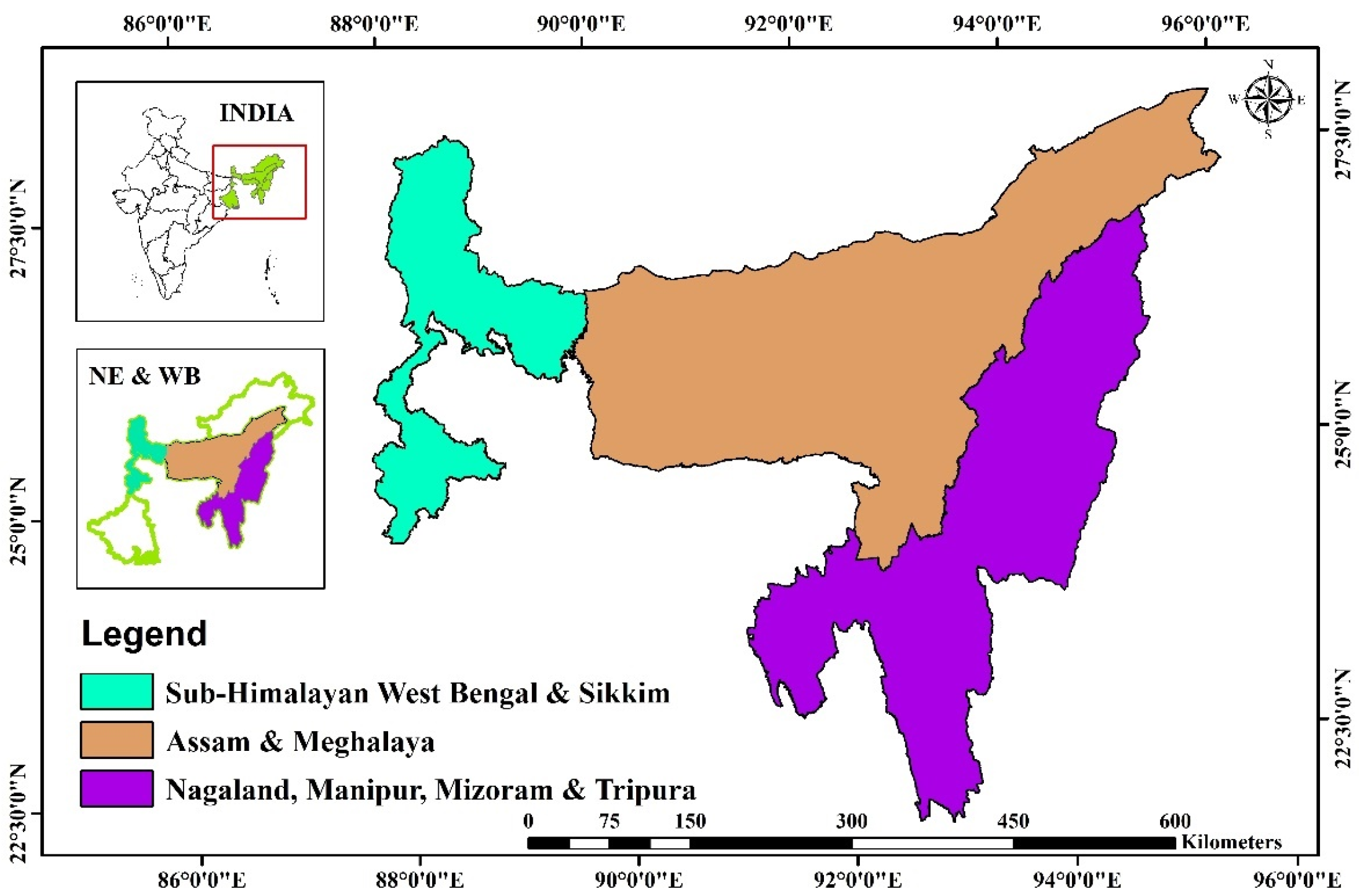
2.1. Study Area

Northeastern India is part of the Himalayan Mountain belt, with complex geological formations due to tectonic movements. The region includes sedimentary rock formations in the Brahmaputra valley, igneous and metamorphic rocks in the hilly regions, and alluvial soils in the plains. The Shillong Plateau, for example, is primarily composed of sedimentary rocks, while the surrounding areas feature a mix of limestone, sandstone, and shale [52] (Govin et al., 2018). The region’s elevation varies from sea level in the plains to over 7000 m in the Himalayas (like in Sikkim). The Shillong Plateau, which is a prominent feature of the region, has an average elevation of about 1500 m above sea level [53] (Sarania et al., 2022). The annual temperature in Northeastern India varies significantly due to the region’s topography. Generally, the lower plains experience warmer temperatures, averaging between 25 °C and 30 °C, while the higher altitudes, particularly in the Himalayan foothills, have temperatures around 10 °C to 15 °C [54] (Saikia et al., 2016). The Köppen classification identifies the region as having tropical wet and dry climates (Aw) in lower altitudes and tropical rainforest climates (Af) in higher elevations [55] (Rao et al., 2016).

2.2. Data Source

This study explored the long-term regional-level climate datasets. The regional level datasets series for the duration of 1871–2016 is a monthly, seasonal, and annual area-weighted rainfall time series for all India, homogeneous regions, and meteorological sub-divisions (MSD) constructed based on a fixed and well-distributed network of 306 rain gauge stations over India [56]. As this study is focused on the northeastern region of India, we have selected Northeastern India (NEI), a homogeneous region, along with three of its meteorological sub-divisions i.e., Assam and Meghalaya (AM i.e., MSD: 3), Nagaland, Manipur, Mizoram and Tripura (NMMT i.e., MSD: 4), and Sub-Himalayan West Bengal and Sikkim (SHWB&S i.e., MSD: 5) (Figure 1). Apart from that, we have also taken the all India (AI) rainfall series so that we can understand the broad pattern in the country-level rainfall vis-à-vis regional patterns.

The time series of climatic variables is analyzed using the appropriate tests to examine monthly, seasonal, and annual trends as well as change points. Seasonal trends were investigated by classifying the calendar year into four distinct seasons, namely January-February (winter), March–May (pre-monsoon), June–September (monsoon), and October–December (post-monsoon), following India Meteorological Department (IMD) standards. To ensure the continuity of the time series data, missing values were substituted with the corresponding monthly averages when necessary. The results are classified into three significance levels: highly significant (*** denoting p ≤ 0.01); significant (** for 0.01 < p ≤ 0.05); and less significant (* for 0.05 < p ≤ 0.1).

2.3. Data Analysis

2.3.1. Methods for Trend Analysis

Various statistical tests can be utilized to detect and measure monotonic trends, categorized into parametric and non-parametric tests. Since climate datasets follow normal as well as non-normal distribution, we have adopted both linear trend (parametric) as well as Mann–Kendall and Spearman rho tests (non-parametric) tests to obtain holistic and robust results.

2.3.2. Mann–Kendall Test

The Mann–Kendall trend test (MKT) is a non-parametric statistical test used to determine if a trend exists in a time series dataset. The test is used when the data are not normally distributed, and there is no assumption of linearity between the dependent and independent variables. The test can be performed on datasets with tied data points.

The Mann–Kendall test calculates a test statistic “S” for the trend in the data, which is calculated as follows:

$$\mathrm{S}=\sum _{\mathrm{i}=1}^{\mathrm{n}}\sum _{\mathrm{j}=1}^{\mathrm{i}-1}\mathrm{s}\mathrm{i}\mathrm{g}\mathrm{n}({\mathrm{x}}_{\mathrm{i}}-{\mathrm{x}}_{\mathrm{j}})$$

(1)

where n is the number of data points; x_j and x_i are the jth and ith observations, and sign is the sign function, which returns −1, 0, or 1 depending on whether the argument is negative, zero, or positive.

2.3.3. Sen’s Slope Estimator

Sen’s slope estimator is a non-parametric method for estimating the slope of a trend in a time series dataset. The method works by calculating the slopes between all pairs of observations in the dataset and then taking the median of these slopes as the estimate of the overall trend. The advantage of this method is that it is resistant to outliers and does not require assumptions about the distribution of the data.

The slope between N pairs of observations is calculated as follows:

$${\mathrm{Q}}_{\mathrm{i}}=\left({\displaystyle \frac{{\mathrm{X}}_{\mathrm{i}}-{\mathrm{X}}_{\mathrm{k}}}{\mathrm{i}-\mathrm{k}}}\right) \mathrm{f}\mathrm{o}\mathrm{r}\mathrm{i}=1,\dots \dots \dots \dots ,\mathrm{N}$$

(2)

The Sen’s slope estimator is then calculated as the median of these slopes. If there is an odd number of slopes, the median is simply the middle slope. If there is an even number of slopes, the median is the average of the two middle slopes. Finally, the non-parametric test is employed to calculate the actual or true slope, which is subsequently validated using a two-sided test within the 100 × (1 − α)% confidence interval [57,58].

2.3.4. Spearman’s Rho Tests (SRHO)

Furthermore, the non-parametric Spearman’s rho test was also performed to verify the results of the MK test. The standardized test statistic (Zd) was likewise calculated as:

$$\mathrm{D}=1-{\displaystyle \frac{6{\sum }_{\mathrm{i}=1}^{\mathrm{n}}{\{\mathrm{R}\left(\mathrm{X}\mathrm{i}\right)-\mathrm{i}\}}^2}{\mathrm{n}({\mathrm{n}}^2-1)}}$$

(3)

$$\mathrm{Z}\mathrm{d}=\mathrm{D}\sqrt{{\displaystyle \frac{\left(\mathrm{n}-2\right)}{\left(1-{\mathrm{D}}^2\right)}}}$$

(4)

where R(Xi) is the corresponding rank assigned for ith observation (Xi) in the time series, and n signifies the length of the time series. Positive and negative values of Zd indicate the increasing and decreasing trend at a 5% significance level. Ho is rejected if |Zd| > 2.08. To account for the regional variability, the threshold for extreme event time series was fixed at the 90% level of confidence.

2.3.5. Ordinary Least Square (OLS) Linear Regression

This is a parametric approach to analyze trends. The OLS regression technique is used to find the line that best fits the data points by minimizing the sum of the squared differences between the observed and predicted values (residuals). The line is used to explain the trend of time series datasets. Here, we have used seasonal and annual rainfall datasets for this purpose. In OLS analysis, positive slope values indicate increasing trends, while negative slope values indicate decreasing trends. A brief account of the advantages and limitations can be found in Pal and Al-Tabbaa (2011) [59].

2.3.6. Innovative Trend Analysis

Şen (2012) [60] introduced the innovative trend analysis (ITA) to identify trends in rainfall time series. Unlike conventional methods like MKT/SRHO and OLS tests, this method has crucial advantages like (a) assumption-free: ITA does not depend on assumptions such as serial autocorrelation or normality, making it robust for various types of time series data; (b) simple interpretation: the graphical representation facilitates easy visualization of trends in the data; and (c) flexibility: it applies to a wide range of time series datasets without stringent requirements of the data characteristics. ITA segments the time series into two halves and arranges them in ascending order, plotting the first half on the X-axis and the second on the Y-axis on a Cartesian coordinate system. A 1:1 line indicates no trend; points above it signifies a positive trend, and points below denote a negative trend. The slope of ITA (SITA) proposed by Şen (2017) [61] discerns trends: positive SITA indicates an increase, while negative SITA shows a decrease. This method has been used to analyze climatic datasets by several researchers [44,62].

2.3.7. Change Point Analysis Techniques

Change/breakpoint detection in the time series of seasonal and annual rainfall is conducted using three distinct change point tests: Pettit’s test, standard normal heterogeneity test (abbreviated as SNHT), and Buishand test (referred to as BHRT). These tests are recommended by the European Climate Assessment and Dataset Project (ECA&D). Detailed descriptions of each test are provided below.

2.3.8. Pettitt Test

This statistical test, proposed by Pettit (1979) [63], is a non-parametric rank test extensively utilized for assessing the presence of sudden changes in climatic time series data. Its utility lies in its sensitivity to detect change points occurring within the middle of a time series [23]. Notably, this test is adept at identifying significant shifts in the mean of a time series even when the precise timing of the change is unknown. The test operates by utilizing the ranks, denoted as r₁, r₂, r₃…r_n and derived from the series Y₁, Y₂, Y₃…Y_n for computing the statistical values [64]:

$$X_k=2\sum _{i=1}^k{r}_i-k\left(n+1\right) k=1,\dots ,n$$

(5)

As per the test’s findings, in the event of a shift or break in the time series occurring in year E, the statistic’s value reaches its maximum or minimum in the vicinity of the year k = E. The critical values of XE are computed following the methodology outlined by Pettit (1979) [63].

$$X_E=max \left|X_k\right| for 1\le k\le n$$

(6)

2.3.9. Standard Normal Homogeneity Test

This statistical test was proposed by Alexandersson (1986) [65]. It was designed to compare the mean of the initial k years of the dataset with that of the subsequent n − k years:

$$T\left(k\right)=k{{\overline{z}}_1}^2+\left(n-k\right){{\overline{z}}_2}^2 k=1,\dots \dots ..,n$$

(7)

where

$${\overline{z}}_1={\displaystyle \frac{1}{k}}{\displaystyle \frac{\sum _{i=1}^k(Y_i-\overline{Y})}{\sigma }}$$

(8)

$${\overline{z}}_2={\displaystyle \frac{1}{n-k}}{\displaystyle \frac{\sum _{i=k+1}^n(Y_i-\overline{Y})}{\sigma }}$$

(9)

Here, $\overline{Y}$ and $\sigma$ represent the mean and standard deviation of the time series, respectively. In the event of a change point or break transpiring in the Kth year, the test statistic T(k) achieves its peak in the vicinity of the year k = K. The computation of the test statistic T₀ is carried out as follows:

$$T_0=max \left(T\left(k\right)\right) for 1\le k\le n$$

(10)

The null hypothesis is rejected when T₀ exceeds a specific threshold, which varies based on the sample size.

2.3.10. Buishand Range Test

Buishand (1982) [66] developed this statistical test. It involves computing the adjusted partial sum that represents the aggregate difference from the mean for the kth observation within a series x₁, x₂, x₃…x_n with a mean ($\overline{X}$), as detailed by Klein Tank (2007) [67].

$$S_0^{*}=0 and S_k^{*}=\sum _{i=1}^k(X_i-\overline{X}) k=1,\dots \dots .,n$$

(11)

In a homogeneous series, the $S_k^{*}$ values tend to oscillate around zero, mirroring the typical distribution of deviations from the mean in a random time series, which spans both sides of the series mean. If the series experiences a break in year K, then $S_k^{*}$ attains a peak (negative shift) or trough (positive shift) close to the year k = K. To assess the statistical significance of the observed shift, the ‘rescaled adjusted range’ R is employed, representing the disparity between the maximum and minimum $S_k^{*}$ values scaled by sample standard deviation:

$$R={\displaystyle \frac{(max{S}_k^{*}-\min S_k^{*})}{s}} 0\le k\le n for\max \&\min separately$$

(12)

Furthermore, to compare the mean and variability of the whole time series, it was divided into two equal parts. Non-parametric techniques, Kruskal–Wallis (KW) test for comparing the central tendency and Fligner-Killeen (FK) test for the variability [68,69,70], were employed. Kolmogorov–Smirnov test was employed to understand the changes in the probability distribution [49]. Furthermore, to understand the change in the return periods of the assured rainfall, it was calculated using the Weibull method [71].

$$T={\displaystyle \frac{(n+1)}{m}}$$

(13)

where T is the return period in years; n is the total number of events, and m is the rank of the event (with the highest value assigned rank 1, second highest rank 2, and so on). The calculation of T was performed in two parts by splitting the entire series of events into two halves. The T for each event in both halves was calculated separately. The calculated T and the events were then plotted on a semi-logarithmic plot for both halves, with T on the x-axis (abscissa) and the events on the y-axis (ordinate). A logarithmic trend line was fitted to the data to obtain the values. The return periods for the 50th and 75th percentiles of the events were estimated for both halves, and the percent change during the recent half compared to the older half was calculated. All these analyses including the statistical tests were performed using the open-source software R (4.0.2) and its integrated development environment (IDE), R-Studio [72].

3. Results and Discussion

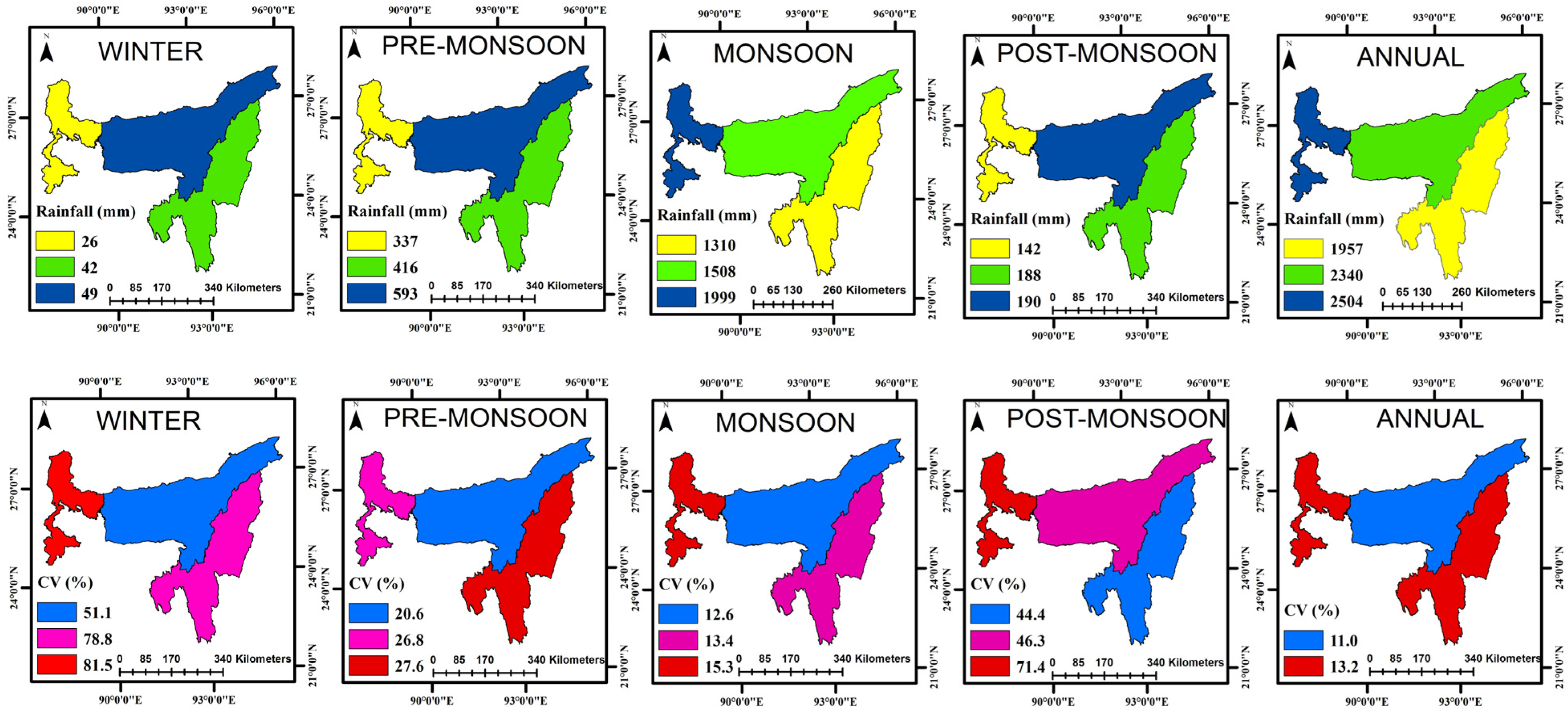
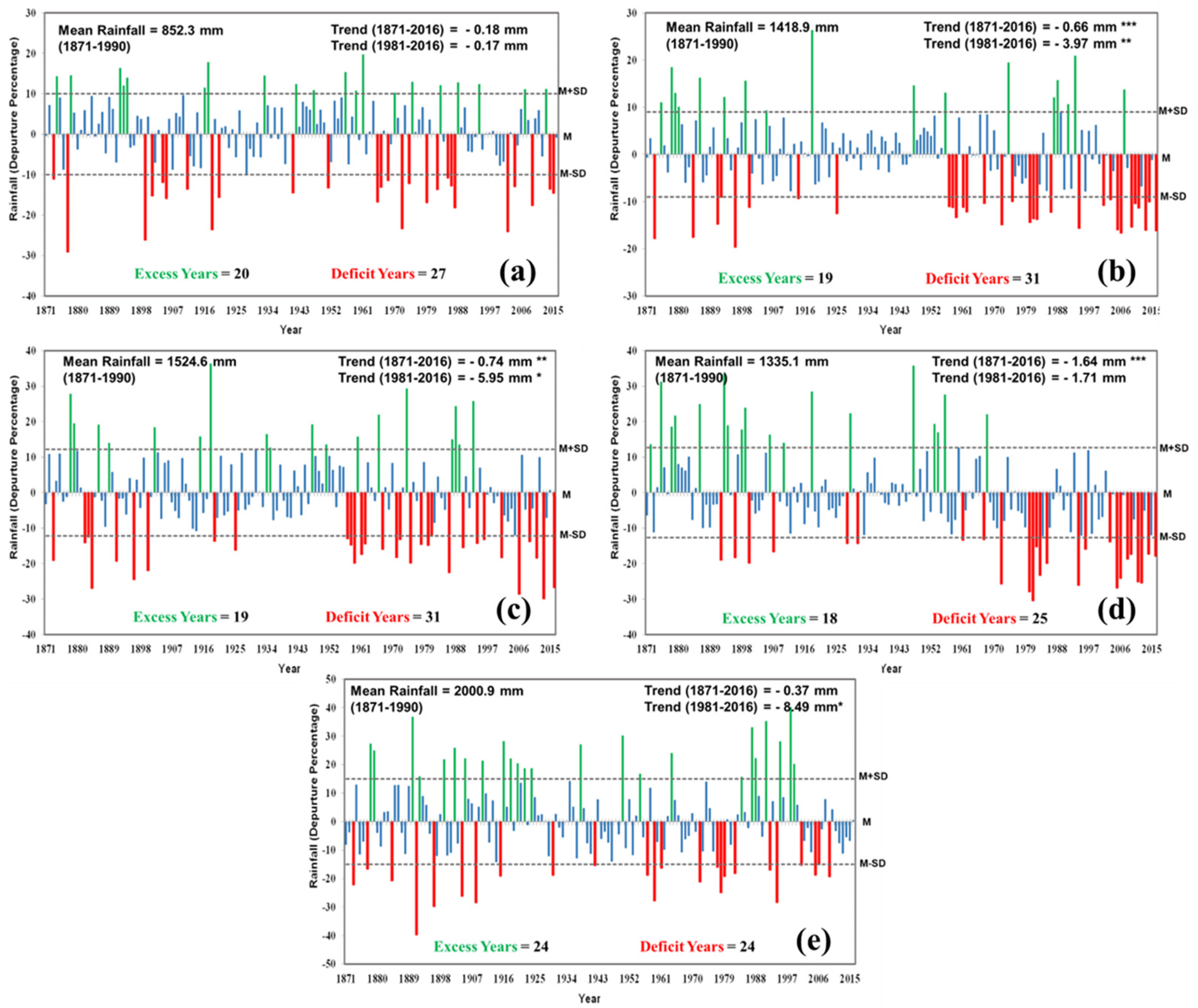
3.1. Summary Statistics of the Rainfall Data

The examination of seasonal rainfall statistics across various regions of India reveals distinctive precipitation patterns. Different statistics like mean, standard deviation (SD), coefficient of variation (CV), minimum (Min), maximum (Max), coefficient of skewness (CS), and coefficient of kurtosis (CK) are provided in Figure 2 and

Table 1. The descriptive statistics of the rainfall (mm) series of the selected regions in India (1871–2016).

		Min	Max	CS	CK
All India (AI)	Winter	3.0	61.1	0.7	3.2
	Pre-Monsoon	55.2	166.5	0.7	3.7
	Monsoon	604.0	1020.2	−0.5	2.9
	Post-Monsoon	50.1	209.9	0.4	2.7
	Annual	810.9	1347.0	0.0	3.1
Northeastern India (NEI)	Winter	0.9	118.2	0.7	3.5
	Pre-Monsoon	226.6	656.5	0.2	2.7
	Monsoon	1139.9	1792.9	0.2	2.9
	Post-Monsoon	26.3	373.8	0.4	2.8
	Annual	1576.4	2504.4	0.0	2.8
Assam and Meghalaya (A&M)	Winter	1.3	149.2	0.7	4.0
	Pre-Monsoon	330.5	1030.5	0.6	3.4
	Monsoon	1068.8	2079.5	0.2	3.0
	Post-Monsoon	51.8	484.9	0.9	3.8
	Annual	1779.9	3102.9	0.2	3.1
Nagaland, Manipur, Mizoram, and Tripura (NMMT)	Winter	0.4	201.2	1.6	6.7
	Pre-Monsoon	142.3	685.3	0.1	2.4
	Monsoon	928.0	1812.8	0.5	3.3
	Post-Monsoon	8.9	429.9	0.4	2.8
	Annual	1406.4	2742.3	0.2	3.0
Sub-Himalayan West Bengal and Sikkim (SHWB&S)	Winter	0.2	112.3	1.5	6.2
	Pre-Monsoon	98.1	650.8	0.8	4.5
	Monsoon	1204.5	2805.7	0.3	2.9
	Post-Monsoon	7.1	565.6	1.2	4.6
	Annual	1705.9	3393.6	0.1	2.9

. It is seen that compared to the AI (1085.9 mm), the NEI (2051.2 mm) received almost double the amount of annual rainfall. There also exist differences in the broad patterns of rainfall among the seasons though in both the cases monsoon season received the highest amount. Monsoon contributed 78% of the total annual rainfall for AI whereas it contributed about 69% in the case of NEI (Figure 3a). After the monsoon season, in the case of AI, the rainfall distribution is post-monsoon (11.1%) > pre-monsoon (8.7%) > winter (2.1%), whereas for NEI, monsoon season was followed by pre-monsoon (20.7%) > post-monsoon (8.6%) > winter (2.1%). It clearly showed that in the case of NEI, the pre-monsoon season received a substantial share of the annual rainfall, and therefore, these months are also very crucial for agricultural activities in the region. In terms of the rainfall amount, for AI, pre-monsoon rainfall was 94.4 mm, whereas for NEI, it was 425.2 mm, which is a substantial quantity for all agricultural operations if the distribution is proper. The rainfall amount during the post-monsoon season was 120 mm for AI and 176.5 mm for NEI. Though the amounts are substantial in these seasons, the rainfall variability during pre- and post-monsoon is quite high both in AI (21.8 and 28.8, respectively) and NEI (19.3 and 40.9, respectively) compared to the monsoon (9.8 and 9.1, respectively). The annual and seasonal values of rainfall in NEI are quite close to those of the Brahmaputra basin [49].

Though the rainfall distribution among the seasons differed, the variability pattern remained the same between AI and NEI (Figure 3b). It can be seen that the lower amount of rainfall was associated with a higher amount of variability. These results signify that though the rainfall amount during pre-monsoon, post-monsoon, and winter may be crucial for agricultural operations, the variability (medium: 20–30%; high >30%), being quite high and assured probability of rainfall being very low, becomes an issue for water/irrigation management planning [73]. Furthermore, the probability of occurrences of the higher side of the extreme also becomes greater, which is further harmful to the crops. Within the NEI, though the broad pattern of rainfall distribution remained similar, (monsoon > pre-monsoon > post-monsoon > winter) the NMMT received a lower amount of rainfall (1956.5 mm) as compared to A&M (2339.8 mm) and SHWB&S (2503.8). Among these regions of NEI, the overall variability was higher in SHWB&S followed by NMMT and minimum in A&M. SHWB&S received the maximum monsoon rainfall (1999.1 mm) which is higher than the other regions. The results are in the range as reported by Jain et al. (2013) [37]. The results indicate that farmers need to be prepared for both floods and droughts, which can occur in any given year. Water resource managers also need to ensure that there is sufficient storage capacity to capture and store monsoon rainfall for use during the dry season.

Most regions and seasons exhibit positive CS values, suggesting longer right tails and indicating the presence of extreme rainfall events. However, NMMT and SHWB&S’s winter season stands out with a higher CS value, indicating a highly skewed distribution with a longer right tail, suggesting more frequent occurrences of extreme winter rainfall events in this region. Deka et al. (2013) [49] reported higher CS for the Barak basin as compared to the Brahmaputra basin. As many parts of the NMMT are under the Barak basin, the results of this study are supported by their findings. Similar to the CS, winter seasons in NMMT (CK = 6.7) and SHWB&S (CK = 6.2) exhibited higher CK values, indicating sharper peaks in the distribution, suggestive of more concentrated rainfall patterns during the winter in these regions. Higher values of CK were also reported by Deka et al. (2013) [49] during the winter seasons over the Barak basin. The results revealed distinct variations in rainfall patterns between AI and NEI as well as within the NEI region. These findings contribute to a better understanding of regional climate characteristics and can inform decision-making processes related to water resource management, agriculture, and disaster preparedness. The regional differences in mean rainfall and seasonal distribution suggest that adaptation strategies to climate change will need to be tailored to specific sub-regions.

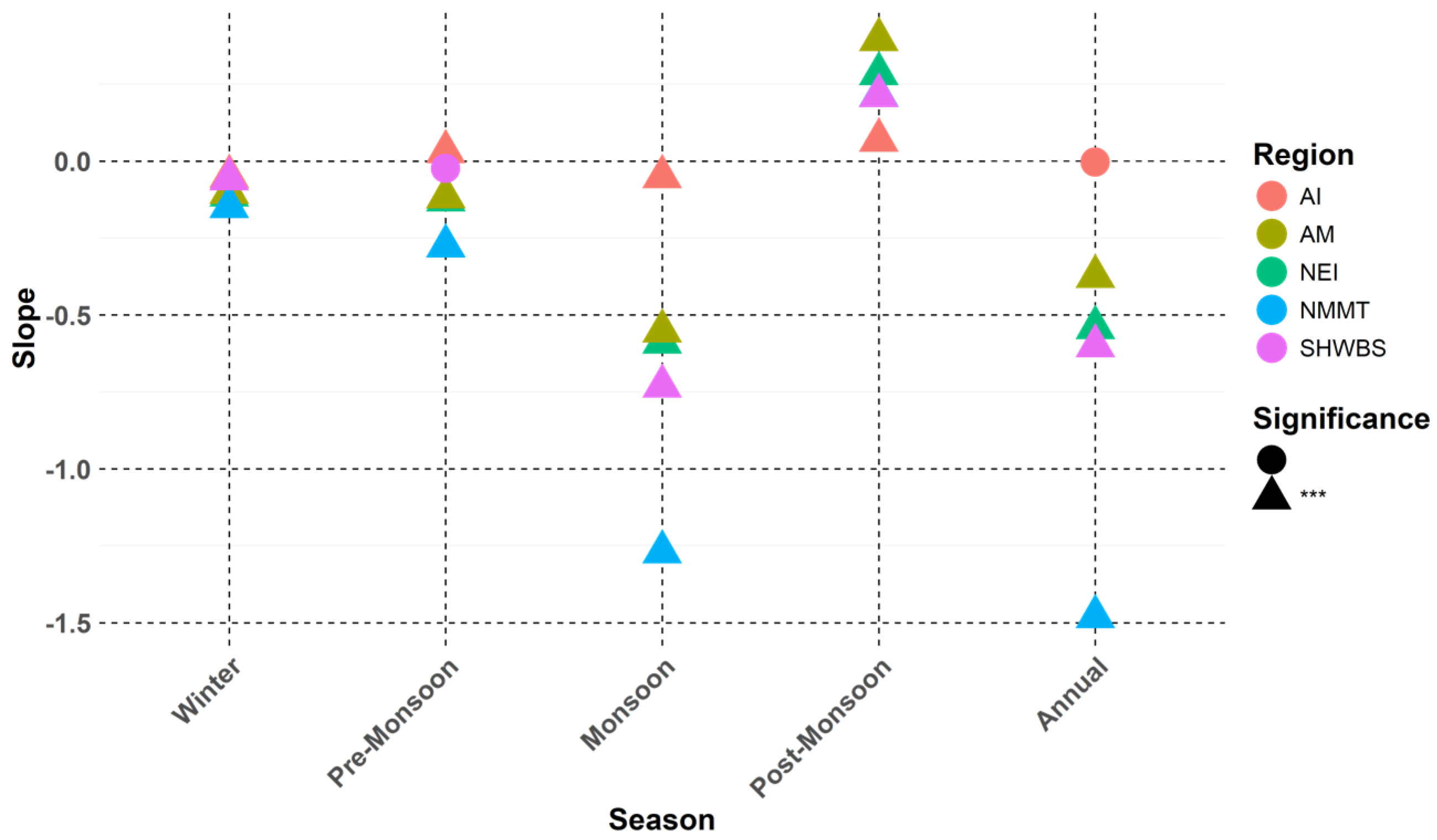
3.2. Trend in the Rainfall Time Series Data

Trends in the long-term rainfall datasets for different regions were tested using the Mann–Kendall test (MKT-Z) and Spearman’s RHO (S-RHO-Zd) for different distinct periods (Full Series: 1871–2016, P1: 1871–1943, and P2: 1944–2016) (Figure 4). The whole time series was divided into two equal parts to understand the periods when the changes were more conspicuous. The results revealed that in the full time series, trends were on the decreasing side for almost all the regions and seasons. However, the values were significant in NEI and within the region in A&M and NMMT. In the case of NEI, a statistically significant decreasing trend was seen in winter and monsoon. Both the statistical tests (MKT and S-RHO) showed similar results, indicating the strength of these results. During P-I, the positive trends mostly dominated in all the selected regions and seasons with only one being statistically significant (winter season in AI), while during P-II, the negative trends dominated completely with many statistically significant values. In the case of AI during winter, monsoon, post-monsoon, and annual time series, the trend was negative but statistically significant during monsoon and annual. For NEI, all the seasons and annual values had decreasing trends with statistical significance during monsoon, post-monsoon, and annual. Within NEI, A&M and NMMT also showed decreasing trends in all the seasons. In the case of A&M, the values were statistically significant during pre-monsoon and monsoon as well as post-monsoon seasons, while for NMMT it was significant during monsoon and annual values. These results indicate that there are negative trends in all the selected regions, and they have become very conspicuous during the latest half of the time series. Another important result is that as compared to the AI, the changes are clearer in NEI. The decreasing trend in rainfall time series at different locations of NEI during winter seasons has been reported by Deka et al. (2013) [49], Saha et al. (2015) [22], Chakraborty et al. (2017) [23], and Marak et al. (2020) [44]. Jain et al. (2023) [51] also reported decreasing trends in the rainfall series of NMMT during monsoon and annual which supports these results. Singh et al. (2021) [62] reported decreasing trends only in winter rainfall in NMMT. However, this study revealed rainfall trends in NEI and its intra-regional variations in a conspicuous manner.

The rate of change was analyzed through the parametric OLS method as well as the non-parametric Sen’s slope method (

Table 2. Rate of change in the rainfall series of the selected regions in India during different periods.

		Full Series (1871–2016)		P-I (1871–1943)		P-II (1944–2016)
		OLS-Slope	Sen-Slope	OLS-Slope	Sen-Slope	OLS-Slope	Sen-Slope
All India	Winter	−0.02	−0.01	0.18 ***	0.21 ***	−0.04	−0.02
	Pre-Monsoon	0.03	0.03	0.02	0.02	0.04	0.01
	Monsoon	−0.18	−0.21	−0.22	−0.41	−0.94 **	−0.93 **
	Post-Monsoon	0.04	0.04	0.15	0.13	−0.22	−0.18
	Annual	−0.13	−0.1	0.13	0.12	−1.15 **	−1.15 *
Northeastern India	Winter	−0.08 *	−0.08 *	0.07	0.1	−0.08	−0.06
	Pre-Monsoon	−0.14	−0.14	−0.1	−0.06	−0.27	−0.07
	Monsoon	−0.66 ***	−0.81 ***	0.01	−0.06	−1.8 **	−2.03 ***
	Post-Monsoon	0.15	0.17	0.33	0.44	−0.85 **	−0.77 *
	Annual	−0.74 **	−0.9 **	0.31	0.06	−3 ***	−3.17 ***
Assam and Meghalaya	Winter	−0.08 *	−0.09 *	0.05	0.06	−0.1	−0.09
	Pre-Monsoon	−0.23	−0.26	0.05	−0.19	−1.19 *	−1.32 *
	Monsoon	−0.74 **	−0.73 **	0.05	−0.25	−2.66 **	−2.84 **
	Post-Monsoon	0.21	0.17	0.44	0.55	−1.16 **	−1.11 **
	Annual	−0.85 *	−0.97 *	0.59	0.24	−5.11 ***	−4.98 ***
Nagaland, Manipur, Mizoram, and Tripura	Winter	−0.13 **	−0.11 **	0.02	0.03	−0.13	−0.11
	Pre-Monsoon	−0.23	−0.26	−0.19	−0.2	0	−0.06
	Monsoon	−1.64 ***	−1.54 ***	−1.57 *	−1.06	−3.93 ***	−3.6 ***
	Post-Monsoon	0.08	0.03	0.2	0.26	−0.87 *	−0.9
	Annual	−1.92 ***	−1.89 ***	−1.54	−1.51	−4.94 ***	−5.3 ***
Sub-Himalayan West Bengal and Sikkim	Winter	−0.04	−0.03	0.07	0.07	−0.03	0.01
	Pre-Monsoon	0.06	0.12	0.52	0.53	0.08	0.37
	Monsoon	−0.37	−0.62	0.94	0.45	0.48	0.3
	Post-Monsoon	0.21	0.23	0.72	0.53	−0.3	−0.2
	Annual	−0.14	−0.37	2.26	1.47	0.23	−0.32

*** for p ≤ 0.01, ** for 0.01< p ≤ 0.05, and * for 0.05 < p ≤ 0.1.

). Similar to the trend test results, these results also revealed a mostly negative rate of changes for the full series while the values were statistically significant in NEI, A&M, and NMMT. The rate of change was highest (decreasing) in NMMT during the monsoon season (more than 1.5 mm/year), which contributed to a more than 1.9 mm/year decrease in the annual values. In the case of A&M, during the monsoon season, the rate of decrease was highest (0.73 mm/year) followed by the winter season. During the P-I, most of the rates of changes were on the positive side, and the changes were not statistically significant. In the case of NMMT, a decreasing rate (1.5 mm/year) was found using the OLS method though Sen’s slope did not detect that as statistically significant. But there were many statistically significant rate changes in P-II, all on the decreasing side. In the case of AI, the decrease in monsoon rainfall was 0.9 mm/year while the decrease in NEI was almost double (1.8 mm/year). In the case of NEI, the rainfall was decreasing in all the seasons, and the rate is slightly higher during the monsoon and post-monsoon seasons. Within the NEI, there are intra-regional variations in the rate of changes. In A&M, the rate of changes was significant, and values were slightly higher during pre-monsoon (1.2 mm/year), monsoon (2.7 mm/year), and post-monsoon (1.1 mm/year), leading to a higher annual change of more than 5 mm/year. In the case of NMMT, during monsoon season, the rate of decrease was the highest (3.9 mm/year). The change in post-monsoon season was also statistically significant using the OLS method. The annual rate of decrease in NMMT was also more than 5 mm/year. Though the direction of the rate of changes matched with some of the earlier studies, the values had differences [51,62]. The results of this study are the outcome of two different statistical tests, thereby indicating the strength of the values.

3.3. Innovative Trend Analysis of the Rainfall Time Series Data

ITA is a statistical test that uses graphical methods to depict the trends in the time series. This study used the ITA test along with the conventional trend tests to understand the patterns. ITA results revealed a decreasing trend in the rainfall for all the selected regions and seasons (Figure 5 and Figure 6). Furthermore, in almost all the cases, it was statistically significant. However, in the case of AI during pre and post-monsoon, the trends were leaning towards an increase and were also statistically significant. But in the case of NEI, during all the seasons, there was a statistically significant decreasing trend except in post-monsoon where it was increasing. A similar pattern was seen in the case for A&M and NMMT, whereas for SHWB&S, the trend was non-significant during pre-monsoon season. The results can also be viewed from the ITA graph (Figure 6), where the points in the upper half indicate an increasing trend, whereas points in the lower half indicate decreasing trends. For the full-time series of the dataset, ITA results in terms of the direction of the trend matched very well with that of the other tests (MKT and S-RHO). However, the test was statistically significant most of the time in the case of ITA (twenty-three out of twenty-five times), whereas for other tests, they were significant for a lower number of cases (nine out of twenty-five). The results of ITA did not match when the time series was divided into two halves. In such cases, during the recent half (P-II), there were mostly decreasing trends, and those were statistically significant even during the post-monsoon season (in NEI and A&M) (Table 2). These results indicated that for a long time series dataset (here 146 years), the ITA is very clearly capable of identifying the overall trend along with its statistical significance, but for relatively shorter periods of the whole series, it faces lacunae compared to the conventional parametric or non-parametric tests. The results of Singh et al. (2021) [62] also clearly indicated that ITA was able to identify the trends more conclusively than other conventional tests. However, they reported a decreasing trend in A&M during winter and pre-monsoon and an increasing trend during monsoons, post-monsoon, and annual, whereas this study found an increasing trend only during the post-monsoon season. Similarly, some mismatches were also identified in the NMMT and SHWB&S regions. These differences may be due to the use of different datasets and the duration of the analysis. Marak et al. (2020) [44] also reported decreasing rainfall trends in two watersheds of Meghalaya through ITA, which supports the findings of this study. These results indicate that for most of the period of the year, there is a decreasing trend in rainfall over the NEI except during the post-monsoon season. Also, within NEI, there are intra-regional differences. The patterns are similar between A&M and NMMT, while it is a bit different in SHWB&S.

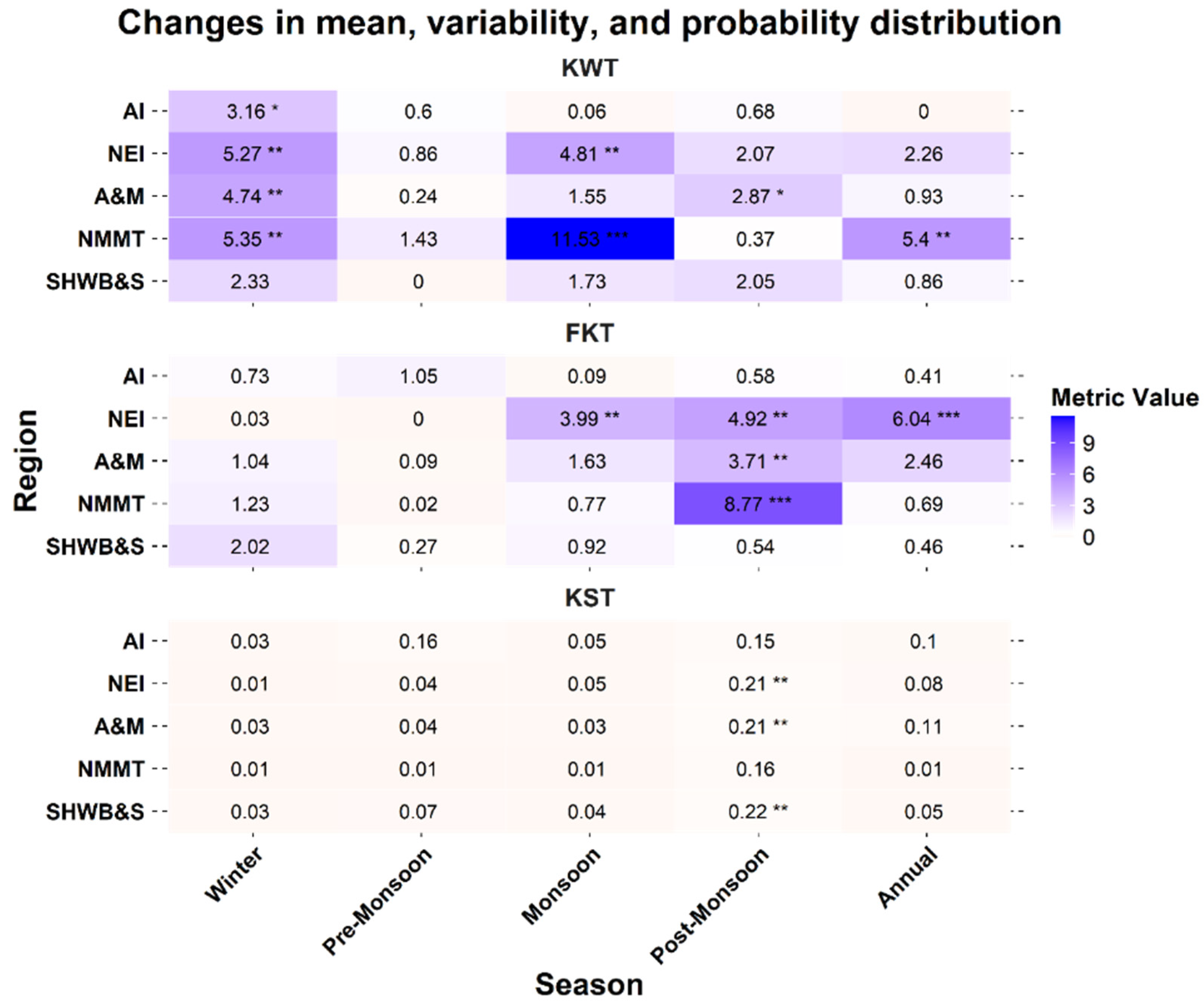
3.4. Changes in Mean, Variability, and Probability Distribution

The trends in the datasets only reflect the changes over time but whether there has been a significant change in different distribution parameters is not revealed. Therefore, we analyzed the datasets with the KW test to understand the changes in the mean (Figure 7). The results indicated that NEI had statistically significant changes during winter and monsoon seasons. Within NEI, in the case of A&M, the changes were significant during winter and post-monsoon while for NMMT, it was significant in winter, monsoon, and annual. However, for SHWB&S, none of the values were significant. Similarly, the FK test was performed to understand the changes in the variability. The results indicated that statistically significant changes were there in NEI during monsoon, post-monsoon, and annual, whereas in A&M and NMMT, it was significant in the post-monsoon, indicating that the variability has significantly changed, and the changes were towards the increasing side. KS test was performed to understand the changes in the probability distribution between the periods. The results indicated that statistically significant values were there during the post-monsoon season in NEI, A&M, and SHWB&S. Though studies reported the changes in the mean and variability in different climatic parameters using these statistical tests, there are no such reports on the regional rainfall of NEI [68,69,70,74]. Therefore, these results indicated that there have been changes in the statistical distribution characteristics of the rainfall series in the NEI. The post-monsoon season followed by the monsoon and winter seasons has been influenced. This means that rainfall variability has increased during these periods in recent times.

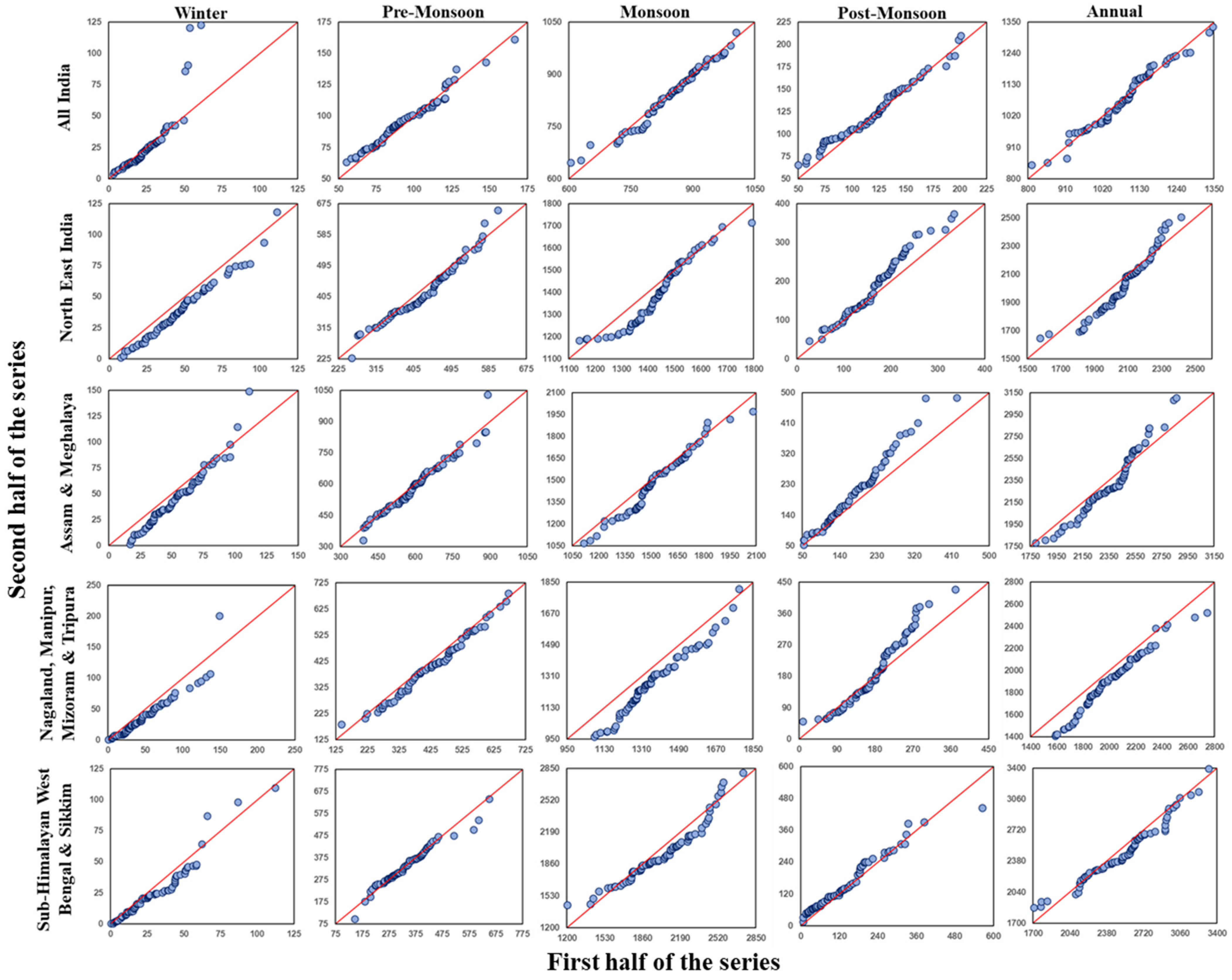
3.5. Change Point Analysis of the Rainfall Time Series Data

The change points in the rainfall time series data were analyzed using three different statistical tests (

Table 3. Change point tests in the rainfall series of the selected regions of India (1871–2016).

		Pettit	SNHT	BHRT
All India	Winter	1948 ***	1948	1949 ***
	Pre-Monsoon	1935 **	2014	1936
	Monsoon	1964 *	1964	1965
	Post-Monsoon	1914 ***	1876	1915
	Annual	1964 ***	1964	1965
Northeastern India	Winter	1945 ***	2008	1946
	Pre-Monsoon	1956 ***	1956	1957
	Monsoon	1956 ***	2000 ***	1957 **
	Post-Monsoon	1908 ***	2005	1945
	Annual	1956 ***	2007 ***	1957 **
Assam and Meghalaya	Winter	1945 ***	2008 ***	1946
	Pre-Monsoon	1959 ***	1959	1960
	Monsoon	1956 ***	2000 ***	1957
	Post-Monsoon	1908 ***	1908	1945
	Annual	1956 ***	2005 ***	1957
Nagaland, Manipur, Mizoram, and Tripura	Winter	1945 ***	1945	1946
	Pre-Monsoon	1895 **	1895	1896
	Monsoon	1969 **	1969 ***	1969 ***
	Post-Monsoon	1891	2010	1946
	Annual	1956 ***	2004 ***	1957 ***
Sub-Himalayan West Bengal and Sikkim	Winter	1945 ***	1962	1963
	Pre-Monsoon	1997	1876	1957
	Monsoon	1939 ***	2000	1940
	Post-Monsoon	1908 ***	1908	1909
	Annual	1956	1873	1957

*** for p ≤ 0.01, ** for 0.01< p ≤ 0.05, and * for 0.05 < p ≤ 0.1.

). The results indicated that Pettit’s test identified the most number of statistically significant change points whereas the number was much lower for SNHT and BHRT. As per Pettit’s test, for AI, the change points occurred in different periods in different seasons, whereas for NEI, the change points for almost all seasons took place during the 1940s to 1950s. The results for monsoon and annual through Pettit’s test also match closely with that of the BHRT while the result for SNHT was varied significantly. The A&M also had almost similar change points to that of the NEI. The results for NMMT matched partially with that of NEI; the change points were similar during winter and annually, while they differed during pre-monsoon and monsoon. Surprisingly, during the monsoon season in NMMT, all three tests indicated the same change point. In the case of SHWB&S, the statistically significant values were during the winter, monsoon, and post-monsoon seasons. It can be seen that during the post-monsoon season, the change points occurred much earlier, and it was the same for NEI, A&M, and SHWB&S. The change point in NEI rainfall data series during winter and annual matched with the values reported by Jain et al. (2023) [51]. This study found that most of the change points in the case of NEI occurred between the 1940s and 1950s, barring a few that occurred either in the 1930s or 1960s. In the case of AI, the change points are a bit scattered from the 1930s to the 1960s. The overall range for the change points matched with the study of Jain et al. (2023) [51] though there were differences as they only focused on the homogenous rainfall regions and not specifically on the MSDs or NEI.

3.6. Trends and Variability in Rainfall Anomalies During the Monsoon Season

In this part of the study, we analyzed the rainfall patterns during the monsoon season as it is the major rainfall season, receiving about 64.4% to 79.8% of the total annual rainfall of the selected regions. The analysis of 146 years of data indicated differences in the broad patterns among the selected regions (Figure 8). There is a large variation in the total monsoon rainfall amount starting from 852.3 mm in AI to 1418.9 mm in NEI. Within the NEI, the NMMT received the lowest (1335.1 mm) followed by A&M (1524.6 mm), and the highest was in SHWB&S (2000.9 mm). The rainfall anomalies varied markedly among these regions (excess indicated by the green color bars and deficit indicated by the red color bars). For AI, there were 20 excess and 27 deficit years, though overall there was a negative trend, but that was statistically non-significant. Compared to that, the NEI faced higher variability in the rainfall as indicated by 19 excess years and 31 deficit years. Even though there is a statistically significant decreasing trend of monsoon rainfall over the whole period (−0.66 mm/year), and the rate of decrease has become six times higher during the last three decades (−3.97 mm/year), the variability has also undoubtedly increased during recent years and after 2000; there have been a total of 10 deficit years over the region as indicated by the red bars. These results indicated that the deficit rainfall anomalies have increased over the NEI at a faster rate in recent time. Our results are in the same line as those reported by Deka et al. (2013) [49], Saha et al. (2015) [22], Chakraborty et al. (2017) [23], and Marak et al. (2020) [44]. Within the NEI, there are lots of variabilities in the inherent rainfall patterns [37]. In consonance with the trend of NEI, all three sub-divisions showed a decreasing trend, and the values are statistically significant. The most striking fact is that, for all the three sub-divisions, the rate of decrease increased rapidly during the last three decades. The rate of decrease was 5.95 mm/year for A&M, 1.71 mm/year for NMMT, and 8.49 mm/year for SHWB&S. These results are supported by the study of Jain et al. (2013) [37] as they reported a decrease during monsoon for all the MSDs of NEI though it was statistically significant only in NMMT. But this study found a statistically significant decrease during the last three decades which Jain et al. (2013) probably missed due to the lack of recent datasets. The increase in variability during the last few decades can easily be seen in Figure 8. Though the negative anomalies mostly dominated in A&M and NMMT, both positive and negative anomalies can be found in SHWB&S sub-division. The deficit anomalies have been very striking during the last two decades over A&M and NMMT, even though the values have often crossed 20% to 30%. The deficit in rainfall in these regions has also been reported by Deka et al. (2013) [49] and Marak et al. (2020) [44], though they did not discuss the variability as such. Furthermore, these anomalies are at the season level, which becomes much more skewed during sub-season levels. Therefore, it can be clearly said that there is a significant negative trend in the monsoon rainfall over the region, and the variability has also increased during recent years. The negative anomalies are rising at a very alarming rate over the region.

3.7. Change in the Return Periods of Assured Rainfall

The change in return periods during the recent half of the time series for assured rainfall probability of 50% and 75% was calculated and is presented in Figure 9. At a glance, the results reveal that the return periods have mostly increased in recent times. In most cases, during the winter season, the return period increased sharply by more than 30%. In pre-monsoon though, for AI, it decreased, but it increased over NEI, especially in NMMT. Furthermore, during monsoon, the main rainfall receiving season, it increased sharply over NEI. Within NEI, the increase was the highest for NMMT followed by A&M and SHWB&S. Post-monsoon season showed a decrease in the return period. Overall, at the annual scale for AI, the change was minuscule, but for NEI, it was quite higher with the highest in NMMT. The increasing return periods of assured rainfall probabilities which are crucial for planning agricultural operations clearly indicate that the assurance of a certain amount of rainfall is decreasing, leading to higher variability [75]. This type of situation poses a threat to the agriculture sector, especially to the prevalent rainfed upland cultivation in Northeastern India.

4. Conclusions

The analysis of long-term rainfall data across India highlights significant distinctions in precipitation patterns, particularly between all India (AI) and Northeastern India (NEI). NEI receives nearly double the annual rainfall compared to AI, with its pre-monsoon rainfall being particularly vital for agriculture. However, high variability in pre- and post-monsoon rainfall in both regions poses challenges for water management and increases the risk of extreme events that are detrimental to crops. Within NEI, regional differences among A&M, NMMT, and SHWB&S further underscore the need for localized adaptation strategies to effectively manage hydro-meteorological hazards. Trend analyses reveal an overall decline in rainfall, particularly during NEI’s winter and monsoon seasons, alongside significant shifts in rainfall patterns in the mid-20th century. Additionally, increasing return periods of assured rainfall exacerbate risks for rainfed agriculture in NEI, highlighting the need for strategic water storage and adaptive agricultural practices. This study emphasizes the growing variability and negative anomalies in monsoon rainfall, which jeopardize agricultural productivity and water resources. Adaptive measures, such as rainwater harvesting and tailored water management strategies, are essential to mitigate the impacts of changing rainfall patterns. Future research should focus on refining region-specific adaptation strategies, using high-resolution climate models, and conducting spatially explicit assessments to ensure informed decision-making for sustainable agriculture and disaster preparedness. The findings provide critical insights for policymakers and stakeholders, offering a foundation for effective planning and resource management in the face of evolving climatic challenges.

References

1. Intergovernmental Panel on Climate Change (IPCC). Summary for Policymakers. In Climate Change 2021—The Physical Science Basis: Working Group I Contribution to the Sixth Assessment Report of the Intergovernmental Panel on Climate Change; Cambridge University Press: Cambridge, UK; New York, NY, USA, 2023; pp. 3–32. [Google Scholar] [CrossRef]
2. Pecl, G.T.; Araújo, M.B.; Bell, J.D.; Blanchard, J.; Bonebrake, T.C.; Chen, I.-C.; Clark, T.D.; Colwell, R.K.; Danielsen, F.; Evengård, B. Biodiversity Redistribution under Climate Change: Impacts on Ecosystems and Human Well-Being. Science 2017, 355, eaai9214. [Google Scholar] [CrossRef] [PubMed]
3. Huang, M.-T.; Zhai, P.-M. Achieving Paris Agreement Temperature Goals Requires Carbon Neutrality by Middle Century with Far-Reaching Transitions in the Whole Society. Adv. Clim. Chang. Res. 2021, 12, 281–286. [Google Scholar] [CrossRef]
4. Li, D.; Wu, S.; Liu, L.; Zhang, Y.; Li, S. Vulnerability of the Global Terrestrial Ecosystems to Climate Change. Glob. Chang. Biol. 2018, 24, 4095–4106. [Google Scholar] [CrossRef]
5. Awasthi, N.; Tripathi, J.N.; Petropoulos, G.P.; Kumar, P.; Singh, A.K.; Dakhore, K.K.; Ghosh, K.; Gupta, D.K.; Srivastava, P.K.; Kalogeropoulos, K. Long-Term Spatiotemporal Investigation of Various Rainfall Intensities over Central India Using EO Datasets. Hydrology 2024, 11, 27. [Google Scholar] [CrossRef]
6. Dore, M.H.I. Climate Change and Changes in Global Precipitation Patterns: What Do We Know? Environ. Int. 2005, 31, 1167–1181. [Google Scholar] [CrossRef] [PubMed]
7. Trenberth, K.E. Changes in Precipitation with Climate Change. Clim. Res. 2011, 47, 123–138. [Google Scholar] [CrossRef]
8. Nielsen, U.N.; Ball, B.A. Impacts of Altered Precipitation Regimes on Soil Communities and Biogeochemistry in Arid and Semi-arid Ecosystems. Glob. Chang. Biol. 2015, 21, 1407–1421. [Google Scholar] [CrossRef]
9. Sun, F.; Roderick, M.L.; Farquhar, G.D. Rainfall Statistics, Stationarity, and Climate Change. Proc. Natl. Acad. Sci. USA 2018, 115, 2305–2310. [Google Scholar] [CrossRef]
10. Gründemann, G.J.; van de Giesen, N.; Brunner, L.; van der Ent, R. Rarest Rainfall Events Will See the Greatest Relative Increase in Magnitude under Future Climate Change. Commun. Earth Environ. 2022, 3, 235. [Google Scholar] [CrossRef]
11. Korner, C.; Spehn, E.M. Mountain Biodiversity: A Global Assessment; CRC Press: Routledge, UK, 2019; Volume 7, ISBN 1000698297. [Google Scholar]
12. Peters, M.K.; Hemp, A.; Appelhans, T.; Becker, J.N.; Behler, C.; Classen, A.; Detsch, F.; Ensslin, A.; Ferger, S.W.; Frederiksen, S.B. Climate–Land-Use Interactions Shape Tropical Mountain Biodiversity and Ecosystem Functions. Nature 2019, 568, 88–92. [Google Scholar] [CrossRef] [PubMed]
13. Schmeller, D.S.; Urbach, D.; Bates, K.; Catalan, J.; Cogălniceanu, D.; Fisher, M.C.; Friesen, J.; Füreder, L.; Gaube, V.; Haver, M. Scientists’ Warning of Threats to Mountains. Sci. Total Environ. 2022, 853, 158611. [Google Scholar] [CrossRef] [PubMed]
14. Sambieni, K.S.; Hountondji, F.C.C.; Sintondji, L.O.; Fohrer, N.; Biaou, S.; Sossa, C.L.G. Climate and Land Use/Land Cover Changes within the Sota Catchment (Benin, West Africa). Hydrology 2024, 11, 30. [Google Scholar] [CrossRef]
15. Achite, M.; Caloiero, T.; Wałęga, A.; Ceppi, A.; Bouharira, A. Trend Analysis of Hydro-Meteorological Variables in the Wadi Ouahrane Basin, Algeria. Hydrology 2024, 11, 77. [Google Scholar] [CrossRef]
16. Rashiq, A.; Kumar, V.; Prakash, O. A Spatiotemporal Assessment of the Precipitation Variability and Pattern and an Evaluation of the Predictive Reliability of Global Climate Models over Bihar. Hydrology 2024, 11, 50. [Google Scholar] [CrossRef]
17. Drenkhan, F.; Buytaert, W.; Mackay, J.D.; Barrand, N.E.; Hannah, D.M.; Huggel, C. Looking beyond Glaciers to Understand Mountain Water Security. Nat. Sustain. 2023, 6, 130–138. [Google Scholar] [CrossRef]
18. Fan, L.; Kuang, X.; Or, D.; Zheng, C. Streamflow Composition and Water “Imbalance” in the Northern Himalayas. Water Resour. Res. 2023, 59, e2022WR034243. [Google Scholar] [CrossRef]
19. Konapala, G.; Mishra, A.K.; Wada, Y.; Mann, M.E. Climate Change Will Affect Global Water Availability through Compounding Changes in Seasonal Precipitation and Evaporation. Nat. Commun. 2020, 11, 3044. [Google Scholar] [CrossRef]
20. Masood, M.U.; Haider, S.; Rashid, M.; Aldlemy, M.S.; Pande, C.B.; Đurin, B.; Homod, R.Z.; Alshehri, F.; Elkhrachy, I. Quantifying the Impacts of Climate and Land Cover Changes on the Hydrological Regime of a Complex Dam Catchment Area. Sustainability 2023, 15, 15223. [Google Scholar] [CrossRef]
21. Chakraborty, D.; Saha, S.; Sethy, B.K.; Singh, H.D.; Singh, N.; Sharma, R.; Chanu, A.N.; Walling, I.; Anal, P.R.; Chowdhury, S.; et al. Usability of the Weather Forecast for Tackling Climatic Variability and Its Effect on Maize Crop Yield in Northeastern Hill Region of India. Agronomy 2022, 12, 2529. [Google Scholar] [CrossRef]
22. Saha, S.; Chakraborty, D.; Choudhury, B.U.; Singh, S.B.; Chinza, N.; Lalzarliana, C.; Dutta, S.K.; Chowdhury, S.; Boopathi, T. Lungmuana Spatial Variability in Temporal Trends of Precipitation and Its Impact on the Agricultural Scenario of Mizoram. Curr. Sci. 2015, 109, 2278–2282. [Google Scholar] [CrossRef]
23. Chakraborty, D.; Saha, S.; Singh, R.K.; Sethy, B.K.; Kumar, A.; Saikia, U.S.; Das, S.K.; Makdoh, B.; Borah, T.R.; Nomita Chanu, A.; et al. Spatio-Temporal Trends and Change Point Detection in Rainfall in Different Parts of North-Eastern Indian States. J. Agrometeorol. 2017, 19, 160–163. [Google Scholar] [CrossRef]
24. Kumar, K.R.; Kumar, K.K.; Ashrit, R.G.; Patwardhan, S.K.; Pant, G.B. Climate Change in India: Observations and Model Projections. In Climate Change and India-Issues, Concerns and Opportunity; Shukla, P.R., Sharma, S.K., Ramana, P.V., Eds.; Tata McGraw-Hill: New Delhi, India, 2002. [Google Scholar]
25. India, G.G.E. Indian Network for Climate Change Assessment; Ministry of Environment and Forests: New Delhi, India, 2010. [Google Scholar]
26. Naresh Kumar, S.; Singh, A.K.; Aggarwal, P.K.; Rao, V.U.M.; Venkateswarlu, B. Climate Change and Indian Agriculture Salient Achievements from ICAR Network Project; Indian Agricultural Research Institute Publications: New Delhi, India, 2012. [Google Scholar]
27. Singh, R.B. Climate Change and Food Security. In Improving Crop Productivity in Sustainable Agriculture; Wiley: Hoboken, NJ, USA, 2012; pp. 1–22. [Google Scholar] [CrossRef]
28. Singh, G. Climate Change and Food Security in India: Challenges and Opportunities. Irrig. Drain. 2016, 65, 5–10. [Google Scholar] [CrossRef]
29. Guhathakurta, P.; Sreejith, O.P.; Menon, P.A. Impact of Climate Change on Extreme Rainfall Events and Flood Risk in India. J. Earth Syst. Sci. 2011, 120, 359–373. [Google Scholar] [CrossRef]
30. Saha, S.; Chakraborty, D.; Paul, R.K.; Samanta, S.; Singh, S.B. Disparity in Rainfall Trend and Patterns among Different Regions: Analysis of 158 Years’ Time Series of Rainfall Dataset across India. Theor. Appl. Climatol. 2018, 134, 381–395. [Google Scholar] [CrossRef]
31. Giri, K.; Mishra, G.; Rawat, M.; Pandey, S.; Bhattacharyya, R.; Bora, N.; Rai, J.P.N. Traditional Farming Systems and Agro-biodiversity in Eastern Himalayan Region of India. In Microbiological Advancements for Higher Altitude Agro-Ecosystems & Sustainability; Goel, R., Soni, R., Suyal, D., Eds.; Rhizosphere Biology; Springer: Singapore, 2020. [Google Scholar] [CrossRef]
32. Majumdar, R.K. State of Biocultural Diversity, Climate Change and Ethnic Meat and Fish Products of Northeast India: A Review. In Impact of Climate Change on Hydrological Cycle, Ecosystem, Fisheries and Food Security; CRC Press: Boca Raton, FL, USA, 2022; pp. 425–437. [Google Scholar]
33. Patra, S.; Rai, S.; Chakraborty, D.; Sangma, R.H.C.; Majumder, S.; Kuotsu, K.; Chakraborty, M.; Baiswar, P.; Singh, B.K.; Roy, A. Impact of Weather Variables on Radish Insect Pests in the Eastern Himalayas and Organic Management Strategies. Sustainability 2024, 16, 2946. [Google Scholar] [CrossRef]
34. Deka, R.L.; Mahanta, C.; Nath, K.K. Trends and Fluctuations of Temperature Regime of North East India. In Proceedings of the ISPRS Proceedings, Impact of Climate Change on Agriculture XXXVIII-8/W3, Cape Town, South Africa, 12–17 July 2009; pp. 376–380. Available online: https://www.isprs.org/proceedings/xxxviii/8-w3/B6/8-45.pdf (accessed on 15 December 2024).
35. Jhajharia, D.; Singh, V.P. Trends in Temperature, Diurnal Temperature Range and Sunshine Duration in Northeast India. Int. J. Climatol. 2011, 31, 1353–1367. [Google Scholar] [CrossRef]
36. Jhajharia, D.; Dinpashoh, Y.; Kahya, E.; Singh, V.P.; Fakheri-Fard, A. Trends in Reference Evapotranspiration in the Humid Region of Northeast India. Hydrol. Process. 2012, 26, 421–435. [Google Scholar] [CrossRef]
37. Jain, S.K.; Kumar, V.; Saharia, M. Analysis of Rainfall and Temperature Trends in Northeast India. Int. J. Climatol. 2013, 33, 968–978. [Google Scholar] [CrossRef]
38. Chakraborty, D.; Singh, R.K.; Saha, S.; Roy, A.; Sethy, B.K.; Kumar, A.; Ngachan, S.V. Increase in Extreme Day Temperature in Hills of Meghalaya: Its Possible Ecological and Bio-Meteorological Effect. J. Agrometeorol. 2014, 16, 147–152. [Google Scholar]
39. Sharma, D.; Das, S.; Goswami, B.N. Variability and Predictability of the Northeast India Summer Monsoon Rainfall. Int. J. Climatol. 2023, 43, 5248–5268. [Google Scholar] [CrossRef]
40. Das, A.; Ghosh, P.K.; Choudhury, B.U.; Patel, D.P.; Munda, G.C.; Ngachan, S.V.; Chowdhury, P. Climate Change in North East India: Recent Facts and Events–Worry for Agricultural Management. In Proceedings of the ISPRS Proceedings, Impact of Climate Change on Agriculture XXXVIII-8/W3, Cape Town, South Africa, 12–17 July 2009; pp. 32–37. Available online: https://www.isprs.org/proceedings/xxxviii/8-w3/B1/2-114.pdf (accessed on 15 December 2024).
41. Dash, S.K.; Kulkarni, M.A.; Mohanty, U.C.; Prasad, K. Changes in the Characteristics of Rain Events in India. J. Geophys. Res. Atmos. 2009, 114. [Google Scholar] [CrossRef]
42. Kumar, S.; Sengupta, K.; Gogoi, B.J. Does Multifaceted Livelihood Intervention Improve Well-being: Reflections on a Case Study from North-eastern India. J. Int. Dev. 2023, 35, 2446–2464. [Google Scholar] [CrossRef]
43. Birthal, P.S.; Khan, T.; Negi, D.S.; Agarwal, S. Impact of Climate Change on Yields of Major Food Crops in India: Implications for Food Security. Agric. Econ. Res. Rev. 2014, 27, 145–155. [Google Scholar] [CrossRef]
44. Marak, J.D.K.; Sarma, A.K.; Bhattacharjya, R.K. Innovative Trend Analysis of Spatial and Temporal Rainfall Variations in Umiam and Umtru Watersheds in Meghalaya, India. Theor. Appl. Climatol. 2020, 142, 1397–1412. [Google Scholar] [CrossRef]
45. Kuttippurath, J.; Murasingh, S.; Stott, P.A.; Sarojini, B.B.; Jha, M.K.; Kumar, P.; Nair, P.J.; Varikoden, H.; Raj, S.; Francis, P.A. Observed Rainfall Changes in the Past Century (1901–2019) over the Wettest Place on Earth. Environ. Res. Lett. 2021, 16, 024018. [Google Scholar] [CrossRef]
46. Prokop, P.; Walanus, A. Variation in the Orographic Extreme Rain Events over the Meghalaya Hills in Northeast India in the Two Halves of the Twentieth Century. Theor. Appl. Climatol. 2015, 121, 389–399. [Google Scholar] [CrossRef]
47. Goswami, B.B.; Mukhopadhyay, P.; Mahanta, R.; Goswami, B.N. Multiscale Interaction with Topography and Extreme Rainfall Events in the Northeast Indian Region. J. Geophys. Res. Atmos. 2010, 115. [Google Scholar] [CrossRef]
48. Varikoden, H.; Revadekar, J. V On the Extreme Rainfall Events during the Southwest Monsoon Season in Northeast Regions of the Indian Subcontinent. Meteorol. Appl. 2020, 27, e1822. [Google Scholar] [CrossRef]
49. Deka, R.L.; Mahanta, C.; Pathak, H.; Nath, K.K.; Das, S. Trends and Fluctuations of Rainfall Regime in the Brahmaputra and Barak Basins of Assam, India. Theor. Appl. Climatol. 2013, 114, 61–71. [Google Scholar] [CrossRef]
50. Paul, A.R.; Maity, R. Future Projection of Climate Extremes across Contiguous Northeast India and Bangladesh. Sci. Rep. 2023, 13, 15616. [Google Scholar] [CrossRef] [PubMed]
51. Jain, S.K.; Xu, C.-Y.; Zhou, Y. Change Analysis of All India and Regional Rainfall Data Series at Annual and Monsoon Scales. Hydrol. Res. 2023, 54, 606–632. [Google Scholar] [CrossRef]
52. Govin, G.; Najman, Y.; Copley, A.; Millar, I.; Van der Beek, P.; Huyghe, P.; Grujic, D.; Davenport, J. Timing and Mechanism of the Rise of the Shillong Plateau in the Himalayan Foreland. Geology 2018, 46, 279–282. [Google Scholar] [CrossRef]
53. Sarania, B.; Guttal, V.; Tamma, K. The Absence of Alternative Stable States in Vegetation Cover of Northeastern India. R. Soc. Open Sci. 2022, 9, 211778. [Google Scholar] [CrossRef]
54. Saikia, P.; Kumar, A.; Khan, M.L. Biodiversity Status and Climate Change Scenario in Northeast India. In Climate Change Challenge (3C) and Social-Economic-Ecological Interface-Building: Exploring Potential Adaptation Strategies for Bio-Resource Conservation and Livelihood Development; Springer: Berlin/Heidelberg, Germany, 2016; pp. 107–120. [Google Scholar]
55. Rao, V.B.; Franchito, S.H.; Gerólamo, R.O.P.; Giarolla, E.; Ramakrishna, S.S.V.S.; Rao, B.R.S.; Naidu, C.V. Himalayan Warming and Climate Change in India. Am. J. Clim. Chang. 2016, 5, 558–574. [Google Scholar] [CrossRef]
56. Kothawale, D.R.; Rajeevan, M. Monthly, Seasonal and Annual Rainfall Time Series for All-India, Homogeneous Regions and Meteorological Sub-Divisions: 1871–2016; Indian Institute of Tropical Meteorology (IITM): Pune, India, 2017. [Google Scholar]
57. Partal, T.; Kahya, E. Trend Analysis in Turkish Precipitation Data. Hydrol. Process. Int. J. 2006, 20, 2011–2026. [Google Scholar] [CrossRef]
58. Malekian, A.; Kazemzadeh, M. Spatio-Temporal Analysis of Regional Trends and Shift Changes of Autocorrelated Temperature Series in Urmia Lake Basin. Water Resour. Manag. 2016, 30, 785–803. [Google Scholar] [CrossRef]
59. Pal, I.; Al-Tabbaa, A. Assessing Seasonal Precipitation Trends in India Using Parametric and Non-Parametric Statistical Techniques. Theor. Appl. Climatol. 2011, 103, 1–11. [Google Scholar] [CrossRef]
60. Şen, Z. Innovative Trend Analysis Methodology. J. Hydrol. Eng. 2012, 17, 1042–1046. [Google Scholar] [CrossRef]
61. Şen, Z.; Şen, Z. Innovative Trend Analyses. In Innovative Trend Methodologies in Science and Engineering; Springer: Berlin/Heidelberg, Germany, 2017; pp. 175–226. [Google Scholar]
62. Singh, R.N.; Sah, S.; Das, B.; Potekar, S.; Chaudhary, A.; Pathak, H. Innovative Trend Analysis of Spatio-Temporal Variations of Rainfall in India during 1901–2019. Theor. Appl. Climatol. 2021, 145, 821–838. [Google Scholar] [CrossRef]
63. Pettitt, A.N. A Non-parametric Approach to the Change-point Problem. J. R. Stat. Soc. Ser. C Appl. Stat. 1979, 28, 126–135. [Google Scholar] [CrossRef]
64. Zarenistanak, M.; Dhorde, A.G.; Kripalani, R.H. Trend Analysis and Change Point Detection of Annual and Seasonal Precipitation and Temperature Series over Southwest Iran. J. Earth Syst. Sci. 2014, 123, 281–295. [Google Scholar] [CrossRef]
65. Alexandersson, H. A Homogeneity Test Applied to Precipitation Data. J. Climatol. 1986, 6, 661–675. [Google Scholar] [CrossRef]
66. Buishand, T.A. Some Methods for Testing the Homogeneity of Rainfall Records. J. Hydrol. 1982, 58, 11–27. [Google Scholar] [CrossRef]
67. Klein Tank, A. EUMETNET/ECSN Optional Programme: European Climate Assessment & Dataset (ECA&D) Algorithm Theoretical Basis Document (ATBD); Version 4, Report EPJ029135 2007; Royal Netherlands Meteorological Institute KNMI: Utrecht, The Netherlands, 2007. [Google Scholar]
68. Ibrahim, B.; Karambiri, H.; Polcher, J.; Yacouba, H.; Ribstein, P. Changes in Rainfall Regime over Burkina Faso under the Climate Change Conditions Simulated by 5 Regional Climate Models. Clim. Dyn. 2014, 42, 1363–1381. [Google Scholar] [CrossRef]
69. Harley, C.D.G. Climate Change, Keystone Predation, and Biodiversity Loss. Science 2011, 334, 1124–1127. [Google Scholar] [CrossRef] [PubMed]
70. Chakraborty, D.; Sehgal, V.K.; Dhakar, R.; Varghese, E.; Das, D.K.; Ray, M. Changes in Daily Maximum Temperature Extremes across India over 1951–2014 and Their Relation with Cereal Crop Productivity. Stoch. Environ. Res. Risk Assess. 2018, 32, 3067–3081. [Google Scholar] [CrossRef]
71. Te Chow, V. Handbook of Applied Hydrology: A Compendium of Water-Resources Technology; McGraw-Hill Company: New York, NY, USA, 1964. [Google Scholar]
72. Chakraborty, D.; Sehgal, V.K.; Dhakar, R.; Ray, M.; Das, D.K. Spatio-Temporal Trend in Heat Waves over India and Its Impact Assessment on Wheat Crop. Theor. Appl. Climatol. 2019, 138, 1925–1937. [Google Scholar] [CrossRef]
73. Hare, W. Assessment of Knowledge on Impacts of Climate Change–Contribution. Arctic 2003, 100, 25–35. [Google Scholar]
74. Mazdiyasni, O.; AghaKouchak, A.; Davis, S.J.; Madadgar, S.; Mehran, A.; Ragno, E.; Sadegh, M.; Sengupta, A.; Ghosh, S.; Dhanya, C.T. Increasing Probability of Mortality during Indian Heat Waves. Sci. Adv. 2017, 3, e1700066. [Google Scholar] [CrossRef]
75. Sattar, A.; Khan, S.A.; Banerjee, S. Assured Rainfall Analysis for Enhanced Crop Production under Rainfed Condition in Bihar. J. Agrometeorol. 2018, 20, 332–335. [Google Scholar] [CrossRef]
Figure 1. Map of the study area covering Northeastern India and its three meteorological sub-divisions.
Earth 06 00002 g001
Figure 2. The mean (upper row) and coefficient of variation (lower row) of rainfall in the study regions of India (1871–2016).
Earth 06 00002 g002
Figure 3. Rainfall distribution among the seasons as a percentage of the selected region’s annual rainfall (a) and their seasonal coefficient of variation (CV) (b).
Earth 06 00002 g003
Figure 4. Trends (a: MKT and b: SRHO) in the rainfall series of the selected regions in India during different periods. *** for p ≤ 0.01, ** for 0.01< p ≤ 0.05, and * for 0.05 < p ≤ 0.1.
Earth 06 00002 g004
Figure 5. Innovative trend analysis (p < 0.01) of the rainfall series of the selected regions of India (Upward facing triangle indicated by “***” means statistically significant change while circle indicates non-significant values).
Earth 06 00002 g005
Figure 6. Innovative trend analysis of the rainfall time series datasets (1871–2016) in the selected study regions.
Earth 06 00002 g006
Figure 7. The changes in different characteristics of the rainfall series of the selected regions of India between the two periods (P1: 1871–1943 and P2: 1944–2016). *** for p ≤ 0.01, ** for 0.01< p ≤ 0.05, and * for 0.05 < p ≤ 0.1.
Earth 06 00002 g007
Figure 8. The trend and variability in summer monsoon (JJAS) rainfall (1871–2016) in the selected study regions (AI-(a); NEI-(b), A&M-(c), NMMT-(d), and SHWB&S-(e); mean-M, standard deviation-SD; ***, **, and * denote trends at 1%, 5%, and 10% significance levels; green, red, and blue lines indicates excess, deficit and normal rainfall years, respectively; solid line and dotted lines represent the mean and deviation from mean, respectively).
Earth 06 00002 g008
Figure 9. Percent change in return period of rainfall at different probability levels.
Earth 06 00002 g009