Characterization of the Planetary Boundary Layer Height in Huelva (Spain) During an Episode of High NO₂ Pollutant Concentrations

Abstract

This study investigates the estimation of the boundary layer height (PBLH) in Huelva, Spain, in November 2023, using different methods: Richardson number, humidity gradient and refractivity gradient. From the virtual potential profiles of temperature and specific humidity, in the case of daytime PBLH, which method works best in some situations when there are discrepancies between results is discussed. The results are then compared with the PBLH values obtained from the ERA-5 reanalysis. The synoptic analysis shows that the decrease in PBLH in the central weeks of the month is compatible with a thermal inversion by subsidence due to a persistent anticyclonic situation. Regarding air quality, the NO₂ concentrations in the air quality station of Matalascañas, which is a background station, show negative correlations with the PBLH.

1. Introduction

The concentration of pollutants in the atmosphere is one of the main problems of modern society [1,2] and has an impact on human health [3], climate change [4] and the physics and chemistry of the atmosphere [5]. Both anthropogenic activities such as industry or traffic, and natural emissions such as dust of natural origin generated in arid or semi-arid areas, contribute to poor air quality [6,7]. In addition to pollutants such as aerosols, PM₁₀ or PM_2.5, or gases such as NO₂, O₃, SO₂ or CO that have been monitored for years, there is more recent concern about the effects of other pollutants such as benzene, benzo[a]pyrene, H₂S, NH₃, heavy metals or ultrafine particles. As a reference, the European Union has approved new air quality regulations, the European Directive 2024/2881/EC, that will include more new pollutants compared to the current ones, the European Directive 2008/50/EC, and less permissive limits, together with a series of actions to be carried out by member states with the aim of improving air quality for European citizens.

The concentration of pollutants is determined not only by the emissions injected into the atmosphere, but also by the conditions of the environment in which they are dispersed, namely the atmospheric conditions [8]. The dispersion of pollutants is conditioned at a meteorological level fundamentally by three factors: large-scale meteorological factors such as the presence of persistent anticyclones that inhibit vertical dispersion [9]; atmospheric stratification for vertical dispersion [8,9], such as when thermal inversions occur; and horizontal wind modifications by topography, roughness and local effects such as when pollutants are transported by sea breezes or drainage winds [10,11,12]. In the vertical, pollutants are dispersed mainly in the atmospheric/planetary boundary layer (ABL/PBL), which is the lowest layer of the troposphere that is directly affected by surface forcings and extends from a few meters to 1 or 2 km from the ground [13]. This layer responds to terrestrial forcings with a time scale of one hour or less. The height of the atmospheric boundary layer is one of the parameters that determines the concentration of pollutants, since it defines the layer in which pollutants are mixed [8]. The height of this layer basically depends on the latitude, the time of year, and the time of day [14,15]. This height is defined usually as the altitude of the inversion level separating the free atmosphere from the planetary boundary layer [13].

There are different methods to determine the atmospheric boundary layer height [16,17]. In this work, the Richardson number, the humidity gradient and the refractivity gradient methods calculated from radiosonde information [18] were used. The study is applied over the region of Huelva (Spain), in the southwest part of the Iberian Peninsula during episodes with high concentrations of pollutants. Discussion is based on the results of the different methods used for the PBLH analysis and the visual inspection of vertical profiles of the atmosphere for episodes with high levels of pollutants.

This research paper is novel because it is the first time that an analysis of the height of the boundary layer has been carried out with interest in its effects on air quality in Huelva (Spain), a major industrial hub in southern Spain. The findings provide new evidence highlighting the critical role of meteorological factors and planetary boundary layer height (PBLH) estimation in shaping air quality levels.

2. Materials and Methods

This section provides information about the episodes and data used in the analysis, the main characteristics of the region of Huelva, the region of interest and finally the methodology to calculate the PBLH. The section is subdivided into area characteristics (Section 2.1), data (Section 2.2), episode selection (Section 2.3) and methodology to calculate the PBLH (Section 2.4).

2.1. Area Characteristics

Huelva has a population of around 145,000 and it is located along the Gulf of Cadiz coast in the mouth of the Odiel and Tinto Rivers, in the south-west of Spain (Figure 1). Huelva has a Subtropical-Mediterranean climate with Atlantic influence (Azores anticyclone, Figure 1) characterized by dry and hot summers and wet and mild winters. Temperatures higher than 40 °C are usually reproduced in summer. The highest wind velocity is reproduced during the sunset and episodes of severe gale (force 9 in the Beaufort scale) affect the region occasionally during the year.

In the city of Huelva and its metropolitan area coexist the core of the population of the province of Huelva, greenhouse zones, nature reserves (very near Doñana Park) and one of the most important industrial poles in the South of Spain. In this sense, the city of Huelva is an example of a city influenced by complex industrial emissions [19]. In an area of approximately 10 km around the city and specifically located close to the southern part of the city, numerous and different industries that inject emissions into the atmosphere coexist (chemical and petrochemical complexes, phosphate industry for fertilizer production, harbor operations and a Cu-smelter mainly). Predominant wind directions from south-southwest can significantly influence the air quality of Huelva [19]. Furthermore, typically during the spring and summer seasons, Saharan dust intrusion affects Huelva [20,21] contributing to an increase in the particulate matter levels [22]. Over the last few decades, a lot of studies have investigated the air quality in the region and the contribution of the different industrial sources to the levels of different pollutants [23,24,25,26,27,28].

2.2. Data Sources

2.2.1. Data from Air Quality Stations

To carry out the episode selection, data from official air quality stations (Figure 1) managed by the Sustainability, Environment and Blue Economy Council of the Regional Government of Andalucía (Network of Vigilance and Control of Air Quality), in collaboration with CIQSO (Center for Research in Sustainable Chemistry, Huelva, Spain) of UHU (University of Huelva) who provided the data, were used. Hourly data for November 2023 were analyzed. This month was selected because typically maximum concentrations occur during autumn (and summer), favored by the impact of industrial plumes in breezes [29]. Over the last few decades, industrial emissions were reduced associated with changes in the legislation and cleaner technologies which have contributed to an improvement in the air quality (i.e., for SO₂ [29]). The year 2023 was selected as the most recent year when we carried out the research.

The difficulty of establishing correlations between the PBLH and contamination episodes is due to pollutant dispersion being influenced by atmospheric conditions, source characteristics, buildings and other obstacles [30], causing a non-linear relationship between emissions and concentrations [31]. To minimize the effect of specific emissions, NO₂ concentrations were analyzed in Matalascañas, which is a background station near Doñana’s Park, a Nacional Park and protected area. The main source of NO₂ is traffic, so the increase in this should not influence a background station so directly, and thus, the effect of specific emissions of the pollutant would be minimized. Other stations in the region are more affected by traffic and/or industrial emissions.

2.2.2. Data from Radiosondes

Upper-air meteorological measurements are obtained from radiosonde launches performed by AEMET (the National Spanish Meteorological Agency, Spain) from their site in the city of Huelva (Figure 1). AEMET launches the radiosondes automatically two times per day, approximately at 00 and 12 UTC (for the episode selected local time corresponds to UTC + 1) and it provides information about the vertical profile of the atmosphere. This radiosounding has been operating since December 2018. Information from meteorological instruments coupled in the radiosonde was downloaded from the METEOCIEL web page (https://www.meteociel.fr/observations-meteo/sondage.php?map=1, accessed on 1 December 2024). The radiosonde instruments record atmospheric variables such as temperature (°C), dew point (°C), relative humidity (%), wind speed (m s⁻¹), wind direction (°), or barometric pressure (hPa) from the surface to an altitude of approximately 30 km. All these values are used, mainly, by numerical weather prediction models to represent the initial state of the atmosphere.

2.2.3. Data from Reanalysis

ERA-5 (https://www.ecmwf.int/en/forecasts/dataset/ecmwf-reanalysis-v5, ECMWF Reanalysis v5, accessed on 1 December 2024) is a fifth-generation atmospheric reanalysis produced by ECMWF’s Copernicus Climate Change Service (European Center for Medium-Range Weather Forecasts). This reanalysis covers the Earth in a 31 km grid step, and resolves meteorological variables at 137 levels, up to an altitude of 40 km and since January 1940. The PBLH data from ERA5 were used in this study, which is calculated using the Richardson method with a critical value of Ri_bc = 0.25 [32]. The available values are the daily maximum, mean and minimum values.

2.3. Episode Selection

The month of November 2023 in the Huelva area was characterized by high pressure and stability. Although the month began with a decrease in atmospheric pressure and the passage of several cold fronts, from November 5th onwards, the Azores anticyclone approached the Iberian Peninsula, and its center was established over it. Between November 8th and 9th, a cold front crossed the city and left some precipitation, and then the pressure increased again. Although the center of the anticyclone moved northwards, the high-pressure regime on the surface continued until November 26th, when the pressure began to decrease. The establishment of the Azores anticyclone near the Iberian Peninsula guaranteed stability and prevented the entry of storms that could arrive from the Atlantic. Because of this, hardly any precipitation was recorded in the central weeks of November (Figure 2).

Figure 2 shows some meteorological variables in the month of November from the El Arenosillo station, the closest to the radiosondes with complete data recording. The data was obtained from AEMET open data (https://opendata.aemet.es/centrodedescargas/productosAEMET? accessed on 1 December 2024). The graphs show how the days with non-zero precipitation coincide with the days of a decrease in the maximum daily atmospheric pressure at the surface. In addition, the increase in the average wind speed and gusts coincide with this pressure decrease and with the passage of fronts. The wind speed values, and therefore the horizontal dispersion values, barely exceeded 3 m/s during the central days of November; that is, from when the Azores anticyclone moves towards the Iberian Peninsula and the high-pressure regime is established at the surface. The wind gusts followed a similar trend to that of the average hourly temperature, although on November 21st there was a maximum that coincided with the passage of a front through the study area. Therefore, at a synoptic level, the month of November would be characterized by high pressure due to the effect of the Azores anticyclone and its movement towards the east of the Atlantic. The persistence of high pressures forms a subsidence inversion that reduces the height of the boundary layer; that is, it reduces the volume of air that connects with the surface and feels its forcing. In the following sections, this height will be estimated; however, this height is not always defined in such a way that we can calculate it using the methods available. In situations of low pressure or in other situations where upward movement is forced, such as during the passage of fronts, the air at the surface can rise to very high levels of the troposphere. In these cases, the height of the boundary layer cannot be estimated using the usual methods, and its definition does not make sense. On some days with clouds, the height of the base of the clouds is usually used to estimate it [13]. In order to eliminate this type of situation, in our study, we excluded the days on which the total daily precipitation collected was greater than 2 mm and the average daily wind was greater than 10 m/s. Therefore, November 2nd, 29th and 30th were excluded.

2.4. PBLH Estimation

There are several methods for PBLH estimation, including the Holzworth or parcel method, the Richardson number method, the gradient method and the turbulent kinetic energy method [33,34]. Among the possible estimation methods from a radiosonde, two gradient methods and the Richardson number method were selected. The former focuses on the gradients observed due to an already-formed PBL at its top; the latter considers the atmosphere’s ability to create turbulence. Furthermore, the humidity gradient method and the Richardson number method allow for the analysis of each method’s performance by directly analyzing the vertical profiles and the identification of discrepancies between the two, which can be resolved in some cases. For instance, the studies [33,34] found that the Richardson number method worked better in convective boundary layers, while the humidity gradient method performed better for stable cases. In the case of the refractivity gradient method, its analysis in the vertical profile is more complicated because its definition includes several magnitudes, but its advantage lies precisely in this: the inclusion of both temperature and humidity.

2.4.1. Richardson Number

Numerous research papers have used radiosounding measurements to calculate the PBLH [35] and it has become a fully validated methodology [18]. Here, PBLH is calculated from the radiosounding data using the Ri_b (bulk Richardson number) method [16], the same method used in mesoscale meteorological models like WRF [36] in some PBL schemes or parameterizations (i.e., in the YSU scheme [37],) or ERA5 to diagnose the PBL height.

Ri_b is a dimensionless number that relates vertical stability and vertical shear [38]. To calculate it, knowing the wind speed, the potential virtual temperature (previously calculated considering air temperature and relative humidity), and the atmospheric pressure at each altitude is required. This information is provided by the instruments of the radiosoundings. The bulk Richardson number can be defined at height z following the next equation [39]:

$${Ri}_b=\left({\displaystyle \frac{gz}{{\theta }_{v0}}}\right)\left({\displaystyle \frac{{\theta }_{vz}-{\theta }_{v0}}{u_z^2+v_z^2}}\right)$$

(1)

where $g$ is the acceleration due to gravity, ${\theta }_{v0}$ and ${\theta }_{vz}$ are the virtual potential temperature at the surface and height z, respectively, and $u_z,v_z$ are the wind horizontal velocity components at height z. The virtual potential temperature represents the theoretical potential temperature of dry air that would have the same density as most air [40] and is calculated as:

$${\theta }_v=T_v{\left({\displaystyle \frac{p_0}{p}}\right)}^{{\displaystyle \frac{R}{c_p}}}$$

(2)

where $p$ corresponds to the atmospheric pressure, $R$ is the universal constant of the ideal gases and $c_p$ is the specific heat at constant pressure for an ideal gas.

The potential temperature is the temperature that an unsaturated parcel of dry air would have if brought adiabatically and reversibly from its initial state to a standard pressure, $p_0$, typically 1000 hPa [37]. The virtual temperature is the temperature that dry air would have if its pressure and density were equal to those of a given sample of moist air [40].

The threshold number of Ri_b defines the transition from turbulent to laminar state as an indicator of the top of the PBL [13]. PBLH is calculated at the altitude where Ri_b exceeds a critical Richardson number (Ri_bc). In the literature, different critical Richardson numbers were defined [41], with 0, 0.25 and 0.5 being more usual. In this paper, we test different Ri_bc and we compare against the vertical profile of the virtual potential temperature to analyze the most appropriate value for the region of interest during the episodes selected, with the aim to establish correlations between episodes with poor air quality and the PBLH.

2.4.2. Humidity Gradient Method

At the top of the boundary layer, the highest gradients of humidity, temperature and pollutants are found. Therefore, the PBLH can be estimated as the level of the minimum vertical gradient of specific humidity (q) with a significant reduction in atmospheric humidity [42,43]. This method has the disadvantage that the local gradient approach could lead to an ambiguous height determination for scenarios where there is no pronounced inversion layer (deep convective region, residual layer over land, stable PBL) or where the PBL is topped by a cloud layer or where there are multiple layers in the troposphere with strong gradients [43].

2.4.3. Refractivity Gradient Method

Among other methods widely used in the literature is the identification of the minimum gradient of refractivity N, understanding, as in the previous method, the PBL as a more humid, dense and refractive zone than the free atmosphere above [42]. This method [44], used for the first time by [45], has the advantage of combining temperature and humidity profiles, and uses the following definition of refractivity N [42].

$$\mathrm{N}=77.6{\displaystyle \frac{p}{T}}+3.73\times {10}^5{\displaystyle \frac{e}{T^2}}$$

(3)

where $p$ corresponds to the atmospheric pressure, $T$ is temperature and e is the vapor pressure of water.

3. Results

3.1. PBLH Estimation

The methods for estimating the PBLH described in the methodology were applied to the radiosondes of November 2023, both for nighttime values (the 00 h UTC radiosonde) and daytime values (from the 12 UTC launch). The PBLH obtained was studied separately according to daytime and nighttime values.

3.1.1. Daytime Values

During the day, the existence of the mixed layer, i.e., the daytime boundary layer, allows the PBLH to be estimated using the methods presented in the methodology, except for the days ruled out due to the meteorological situation.

The daytime values were analyzed one by one and the values considered most appropriate were selected considering visual estimation. In Figure 3, the shading represents the range of values for the height of the daytime boundary layer considered valid. The blue lines represent the days in which the meteorological situation would have affected the capacity to estimate the daytime boundary layer heights.

During the process of day-per-day PBLH estimation, some discrepancies were identified. The discrepancies between the values obtained using the different methods were analyzed using vertical humidity and temperature profiles. Three types of discrepancies were identified between the methods and these discrepancies define three types of profiles that we named “A-type profiles”, “B-type” and “C-type”. In the next lines, these profiles are analyzed in depth.

• A-type profiles;

The virtual potential temperature profile of the mixed layer is superadiabatic in a deep layer close to the surface. The Richardson and refractivity gradient methods can overestimate the PBLH with respect to the humidity gradient method, especially the Richardson method, with any of the critical values used. It is important to remember that this method recalculates the buoyancy at each level, calculating the virtual potential temperature gradient of that level with respect to that of the surface. On November 6th, the height of the PBL that would coincide with a significant variation in the humidity gradient could be estimated visually from the vertical profiles of virtual potential temperature and specific humidity (Figure 4). On November 6th, the Richardson number and refractivity gradient methods overestimate the PBLH with respect to the humidity gradient method by over 1000 m. We can observe that the mixed layer has a superadiabatic gradient and this gradient compensates for the jump in virtual temperature that represents the top of the PBL. In other profiles with similar situations, it was considered that the method that best estimates the height of the PBL is the humidity gradient method.

• B-type profiles;

From November 8th, the Azores anticyclone approached the Iberian Peninsula and remained over it until the end of November. Due to this persistence and the subsequent subsidence inversion, the height of the boundary layer or mixed layer decreased.

To implement the humidity gradient or refractivity method, the gradient of these variables is calculated at each level, and then the level with the minimum value is selected. However, if the height of the boundary layer is much lower than the maximum level up to which this minimum gradient is sought, it is possible that in the free atmosphere, above the PBL, a humidity gradient is found that is lower than that which represents the top of the boundary layer, which may be due to the presence of clouds, advection of humidity in the free atmosphere or another phenomenon. It is difficult to define the height limit under which to identify the minimum gradient, since the PBLH is precisely the unknown value, and in this impossibility of establishing a standard limit lies the possibility of overestimation of the boundary layer by gradient methods with respect to the Richardson method. In the vertical profiles of 18 November, a PBL of around 500 m would be visually determined (Figure 5), which is well approximated by the Richardson method but not by the gradient methods. This occurs because the height limit established in the algorithm to find the minimum gradient is 2000 m. In cases of low PBLH, as is the case, the algorithm can be found in the space between the end of the PBLH and the height imposed in the algorithm minimum gradients that do not signify the end of the PBLH, but are above it, and thus overestimate the height of the boundary layer. This situation occurred in the days from November 11th to 21st, and it was considered that the Richardson method (in any of the critical values) is the one that best estimates the PBLH.

• C-type profiles;

Another characteristic found in the profiles is the underestimation of the PBLH when using the Richardson critical value 0 compared to the other methods. In situations with C-type profiles, the underestimation of the Richardson number method with critical number Ri_bc = 0 in comparison to the other methods can be as high as the height of the PBL. With Richardson critical value equal to 0, a slight inversion of surface temperature can cause the established threshold to be exceeded, and, therefore, the height to be estimated as the height of the boundary layer. On the other hand, increasing the Richardson critical number allows a more realistic estimate of the PBLH. In the profile of November 9th (Figure 6), it can be observed how the gradient methods and the Richardson method for critical values of Ri_bc = 0.1, Ri_bc = 0.25 and Ri_bc = 0.5 estimate the height of the layer in a similar way, which is located around 1000 m, and the Richardson method with Ri_bc = 0 places it at the first level. In similar situations, when this last critical value places the height of the layer at the first level during the day, this result is dismissed.

3.1.2. Nighttime Values

During the night, the boundary layer changes its characteristics significantly. Thermal turbulence disappears and only dynamic turbulence can exist. In weak wind situations, stable thermal stratification inhibits turbulent movements, and it can be difficult to define a PBLH.

As was carried out with the daytime values, an average was made with the PBLH values calculated for the four Ri_bc critical values and both the average and the range of values were calculated and represented. It can be observed that the values obtained are much lower than the daytime values, with a period at the beginning of the month with a lot of variability (Figure 7). The night profile lacks a mixed layer like the daytime one and therefore gradient methods are not valid methods to estimate the boundary layer height (Figure 8). Therefore, in the night radiosondes, only the Richardson method was implemented with the four critical values that we used with the daytime values.

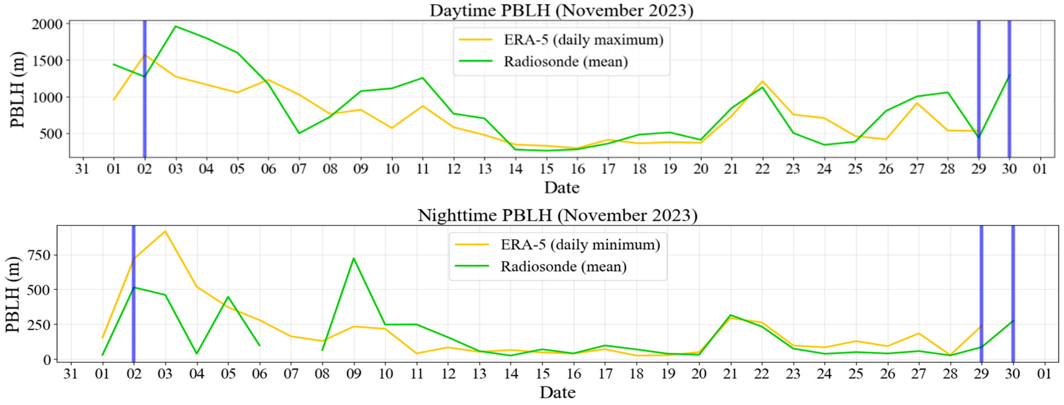
3.2. Comparison Between PBLH Estimation and ERA5

The ERA-5 reanalysis provides daily mean, maximum and minimum values of the PBL height. Figure 9 shows the daytime and nighttime values calculated in the previous sections together with the daily maxima and minima obtained from the reanalysis, respectively. Although it cannot be guaranteed that the PBL reached its maximum height at 12 UTC, in the absence of hourly data, the maximum daily values from ERA5 were compared with the PBL height calculated from the 12 UTC radiosonde, even considering that the error may be considerable. As for the nighttime values, with very weak turbulence, due to their own evolution, the PBLH values remain relatively constant from a few hours after sunset, when they reach their daily minimum. As it cannot be guaranteed that the maximum and minimum values of ERA-5 are from 12UTC and 00UTC, respectively, they are not numerically compared.

In Figure 9, similarities between the two values can be seen; both show a decrease in the boundary layer that would be compatible with the subsidence inversion due to the prevalence of the high-pressure regime. From November 12th to 20th, both sources represent a minimum of the boundary layer, with a small increase peaking on November 21st.

Although ERA5 also assimilates radiosonde observations, the estimated PBLH is calculated directly from the radiosondes. Therefore, ERA5 values were used as a guide to provide strength to the estimates, but the estimations from the radiosonde were considered when comparing the PBLH with NO₂ concentration.

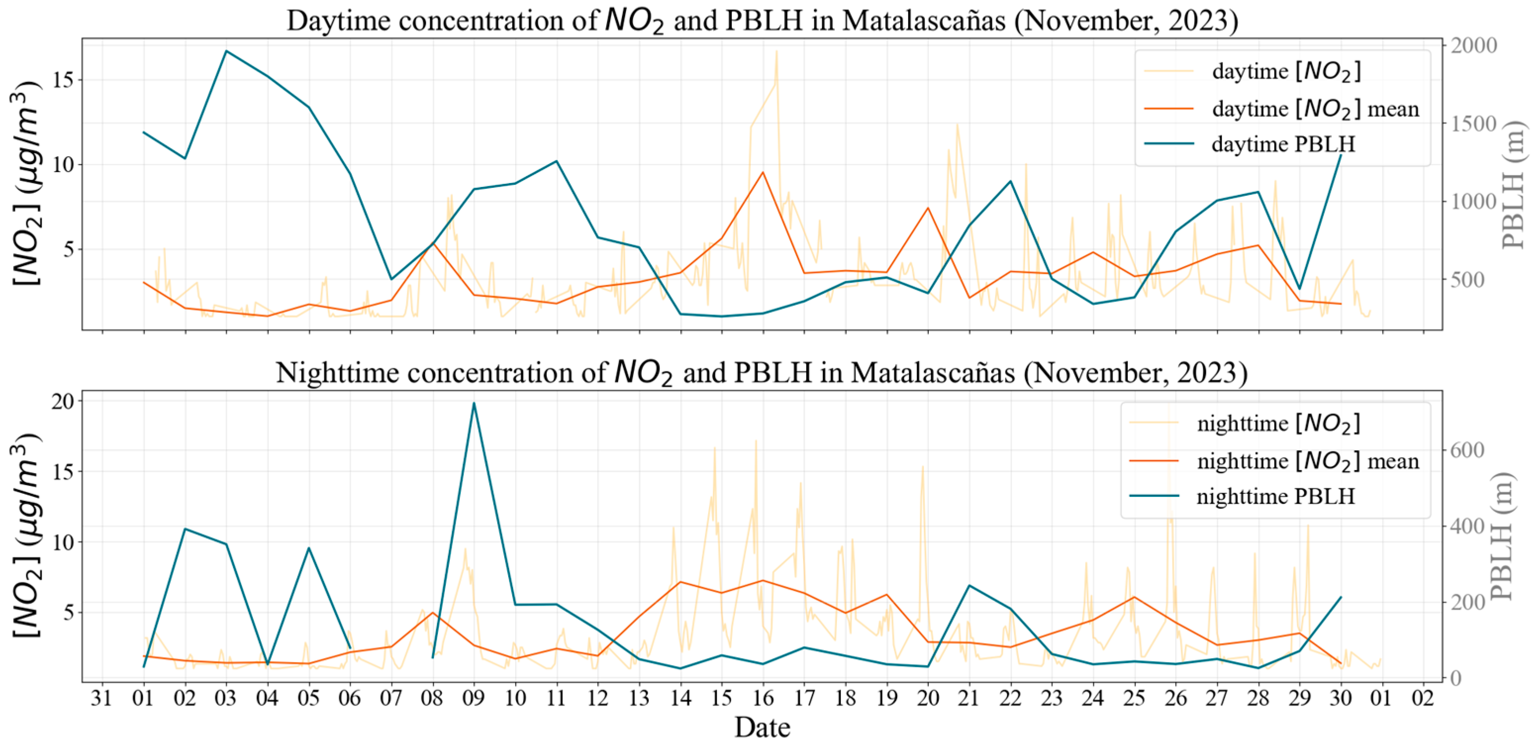
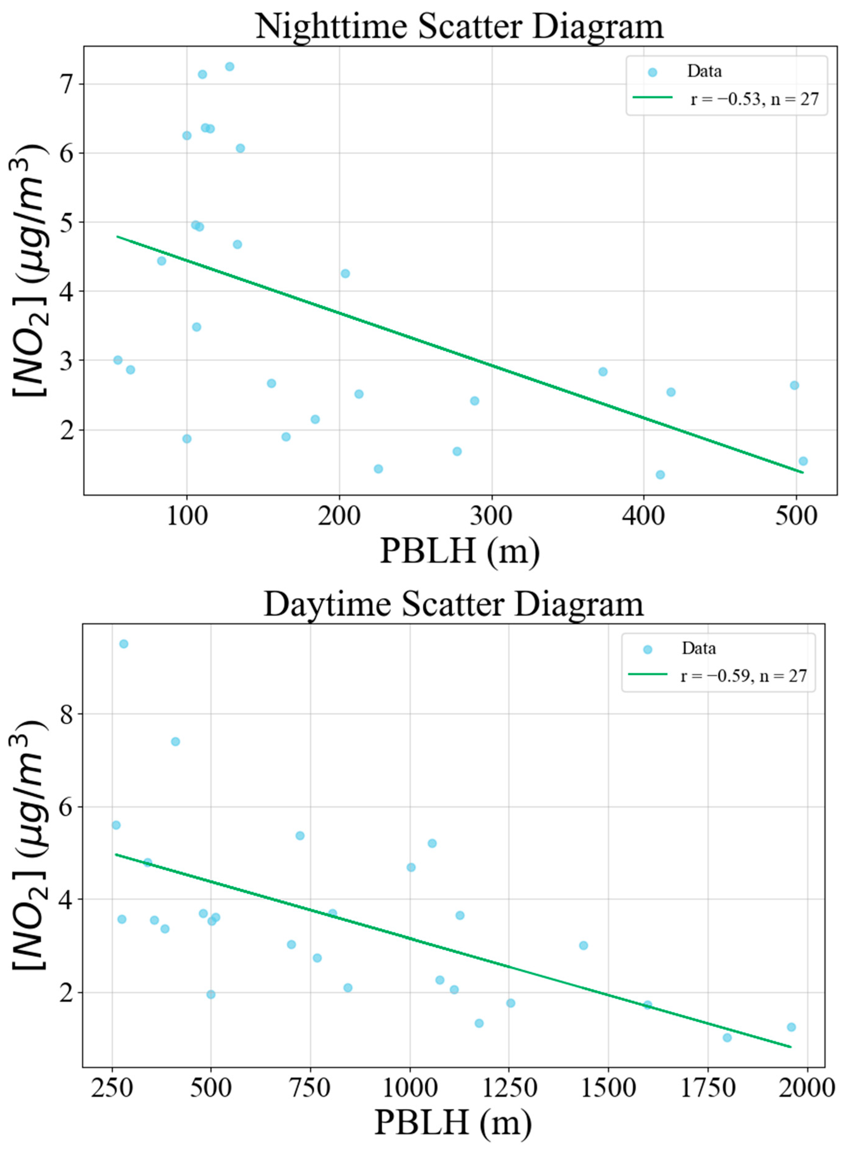
3.3. Correlation Between PBLH and NO₂ Concentration

In Figure 10, the NO₂ values at the Matalascañas station are shown, as well as the corresponding daily averages and the daytime and nighttime PBLH, calculated with the estimations from radiosondes. As expected for a background station, the values are far from exceeding any threshold determined as harmful or dangerous for human health or the environment; however, a notable increase in the concentration of NO₂ can be observed from November 13th, which coincides with the decrease in the PBLH due to the high-pressure situation caused by the Azores anticyclone located over the Iberian Peninsula.

The correlation between the mean mixed layer height and the mean daytime concentration of NO₂ was studied, and, in the daytime scatter diagram, a negative linear correlation of value r = −0.59 can be observed (Figure 11); that is, there is a negative correlation between both variables. Therefore, the decrease in the PBLH would be related to the increase in pollution. In the case of the nighttime data, the correlation is also negative, r = −0.53, somewhat lower than that of the daytime values. In both graphs, it can be observed immediately how the maximum concentration values correspond to lower values of the PBLH. As expected, this occurs because when the PBLH is maximum, the volume where NO₂ can be mixed is maximum, so as concentration is mass per volume unit, the conditions are in place to minimize the NO₂ concentration; vice versa, when PBLH is minimum, the volume where NO₂ can be mixed is minimum, and the conditions to achieve higher concentrations are in place.

4. Discussion

The results reinforce the initial and well-studied hypothesis [14] that atmospheric stable situations such as persistent anticyclonic situations can cause episodes of poor air quality. Although the study methods were used previously in numerous works, the more thorough study of the suitability of each of the methods in some types of vertical profiles can be useful for later works.

Although the relationship between PBLH and poor air quality levels is something that has been widely studied, this study has allowed us to diagnose a practical and useful method to estimate said PBLH. The persistence of an anticyclone could be used as an indicator of a possible decrease in the boundary layer height and, therefore, a possible increase in pollutant concentrations. Although precise models in this field obviously exist today, the use of meteorological analyses jointly with the radiosonde analysis could be very useful. This information is especially relevant for air quality forecasting models that typically are coupled systems combining a meteorological model, emissions information and a dispersion or a photochemical model. In any case, these coupled modelling systems present the difficulty of requiring knowledge of the emissions injected into the atmosphere from the different local, regional and even cross-border emission sources, and therefore, they involve a high amount of effort. The methodology followed allows us to know, at first approximation, the air quality for the next few days only based on meteorological conditions, like how the ventilation conditions or ventilation rate are defined for a certain area [46,47,48]. Ventilation conditions, which are the combination of PBLH and wind velocity, can be used to impose limitations on the emissions allowed into the atmosphere [49] or to help regulate outdoor burning [46,48]. Without pretending to replace the predictive air quality models, this methodology can be a useful tool to predict the air quality in those regions where a complete inventory of atmospheric emissions is not available and, in those points (background), is not directly impacted by nearby emissions.

In future studies, it would be interesting to extend the time range of the study to other months or to other November months in other years, to give more robustness to the comparison of pollution values with those of PBLH. Furthermore, a study of the prevalence of the Azores anticyclone over Huelva or its range of influence could be interesting to determine the frequency of similar situations. Moreover, adding horizontal dispersion to the study could give more robustness to the study and allow other pollutants that have a greater dependence on the emission source to be added to the analysis. Also, analyzing the effects of PBLH over other pollutants will be part of future work, studying the contribution of the PBLH over the levels of these pollutants.

The results obtained in this work can be used to evaluate the performance of meteorological models that can be of interest to the Regional Public Administration or private industries and that can be used as input for photochemical models or dispersion models with the aim of obtaining an air quality forecast. This work can be carried out in other regions where the launch of radiosondes happens and there exists a dense air quality network.

5. Conclusions

A decrease in PBLH can be observed, more noticeable during daytime, in the days following the arrival of the Azores anticyclone on the Iberian Peninsula. Therefore, the low values of the boundary layer during the central days of November can be understood as a result of the persistence of the high-pressure regime. Although the literature shows that PBLH can be difficult to estimate only using radiosonde observations, in a more in-depth analysis of the vertical profiles it was possible to see that depending on the type of vertical profile, some methods are more suitable than others. Of course, the variable to be calculated is the PBLH, and in the absence of actual PBLH data, it cannot be stated that the one proposed as the best estimate is the actual PBLH. Therefore, the study sought to reject PBLH values when, due to the type of situation, the method’s operation could lead to systematic errors. In situations of superadiabatic mixed layer profile, the humidity gradient method may be more suitable than the refractivity gradient and the Richardson method. On the other hand, in situations with a very low and well-mixed PBL, the gradient methods may greatly overestimate the PBLH due to the difficulty of establishing upper limits when implementing the algorithms to find the minimum gradients. The overestimation of the gradient methods in situations with this profile type will depend on the location of vertical gradients within the PBL or in the free atmosphere. The overestimation of the gradient methods in situations with this profile type will depend on the free atmosphere between the top of the planetary boundary layer and the limit that is established in the algorithm when applying the Gradient Methods, and can be greater than 1000 m. Finally, the Richardson method with Ri_be = 0 can consider any surface inversion in the first levels as the end of the boundary layer and underestimate the height of the PBLH as much as the actual height of the PBL. The comparison of the values obtained from the radiosonde with the PBLH values obtained from the ERA-5 reanalysis confirms this decrease in the height of the boundary layer in the central days of November, due to the persistence of the anticyclone over the area.

In the analysis of the pollutant values, it can be observed that the correlation between the PBL height and the mean value of NO₂ concentration is negative in the background pollution station considered, Matalascañas, which shows an inverse correlation of 0.59, although the short period of time does not allow to generalize these results. An extension of the study period, as well as considering the effect of horizontal dispersion jointly with the vertical dispersion within the PBL, would strengthen the results and is undoubtedly a path that future studies could take.

References

1. EEA. How Air Pollution Affects Our Health; European Environment Agency: Copenhagen, Denmark, 2024; Available online: https://www.eea.europa.eu/en/topics/in-depth/air-pollution/eow-it-affects-our-health (accessed on 18 December 2024).
2. WHO. Air Pollution: The Invisible Health Threat; World Health Organization: Geneva, Switzerland, 2024; Available online: https://www.who.int/news-room/feature-stories/detail/air-pollution--the-invisible-health-threat (accessed on 18 December 2024).
3. Newby, D.E.; Manucci, P.M.; Grethe, S.T.; Baccarelli, A.A.; Brook, R.D.; Donaldson, K.; Forastiere, F.; Franchini, M.; Franco, O.H.; Graham, I.; et al. Expert Position Paper on Air Pollution and Cardiovascular Disease. Eur. Heart J. 2015, 36, 83–93. [Google Scholar] [CrossRef] [PubMed]
4. Crutzen, P.J. New Directions: The Growing Urban Heat and Pollution Island Effect-Impact on Chemistry and Climate. Atmos. Environ. 2004, 38, 3539–3540. [Google Scholar] [CrossRef]
5. Ritter, M.; Müller, D.; Tsai, M.-Y.; Parlow, E. Air Pollution Modeling over Very Complex Terrain: An Evaluation of WRF-Chem over Switzerland for Two 1-Year Periods. Atmos. Res. 2013, 132–133, 209–222. [Google Scholar] [CrossRef]
6. EEA (European Environment Agency). Air Quality in Europe 2022; Report No. 05/2022; EEA (European Environment Agency): Copenhagen, Denmark, 2022. [Google Scholar] [CrossRef]
7. Wang, Q.; Gu, J.; Wang, X. The impact of Sahara dust on air quality and public health in European Countries. Atmos. Environ. 2020, 241, 117771. [Google Scholar] [CrossRef]
8. Yuval Tritscher, T.; Raz, R.; Levi, Y.; Levy, I.; Broday, D.M. Emissions vs. turbulence and atmospheric stability: A study of their relative importance in determining air pollutant concentrations. Sci. Total Environ. 2020, 733, 139300. [Google Scholar] [CrossRef]
9. Whiteman, C.D.; Hoch, S.W.; Horel, J.D.; Charland, A. Relationship between particulate air pollution and meteorological variables in Utah’s Salt Lake Valley. Atmos. Environ. 2014, 94, 742–753. [Google Scholar] [CrossRef]
10. Soler, M.R.; Arasa, R.; Merino, M.T.; Ortega, S. Modelling Local Sea-Breeze Flow and Associated Dispersion Patterns Over a Coastal Area in North-East Spain: A Case Study. Bound. Layer Meteorol. 2011, 140, 37–56. [Google Scholar] [CrossRef]
11. Udina, M.; Soler, M.R.; Arasa, R. Effects of nocturnal thermal circulation and boundary layer structure on pollutant dispersion in complex terrains areas: A case study. Int. J. Environ. Pollut. 2012, 48, 47–59. [Google Scholar] [CrossRef]
12. Chemel, C.; Burns, P. Pollutant Dispersion in a Developing Valley Cold-Air Pool. Bound. Layer Meteorol. 2015, 154, 391–408. [Google Scholar] [CrossRef]
13. Stull, R.B. An Introduction to Boundary Layer Meteorology; Kluwer: Dordrecht, The Netherlands, 1988; 670p. [Google Scholar]
14. Sudeepkumar, B.L.; Babu, C.A.; Varikoden, H. Atmospheric boundary layer height and surface parameters: Trends and relationships over the west coast of India. Atmos. Res. 2020, 245, 105050. [Google Scholar] [CrossRef]
15. Peng, S.; Yang, Q.; Shupe, M.D.; Xi, X.; Han, B.; Chen, D.; Dahlke, S.; Liu, C. The characteristics of atmospheric boundary layer height over the Arctic Ocean during MOSAiC. Atmos. Chem. Phys. 2023, 23, 8683–8703. [Google Scholar] [CrossRef]
16. Banks, R.F.; Tiana-Alsina, J.; Rocadenbosch, F.; Baldasano, J.M. Performance Evaluation of the Boundary-Layer Height from Lidar and the Weather Research and Forecasting Model at an Urban Coastal Site in the North-East Iberian Peninsula. Bound. Layer Meteorol. 2015, 157, 265–292. [Google Scholar] [CrossRef]
17. García-Dalmau, M.; Udina, M.; Bech, J.; Sola, Y.; Montolio, J.; Jaén, C. Pollutant concentration changes during the COVID-19 lockdown in Barcelona and surrounding regions: Modification of diurnal cycles and limited role of meteorological conditions. Bound. Layer Meteorol. 2022, 183, 273–294. [Google Scholar] [CrossRef]
18. Kotthaus, S.; Bravo-Aranda, J.A.; Collaud Coen, M.; Guerrero-Rascado, J.L.; Costa, M.J.; Cimini, D.; O’Connor, E.J.; Hervo, M.; Alados-Arboledas, L.; Jiménez-Portaz, M.; et al. Atmospheric boundary layer height from ground-based remote sensing: A review of capabilities and limitations. Atmos. Meas. Tech. 2023, 16, 433–479. [Google Scholar] [CrossRef]
19. Querol, X.; Alastuey, A.; De la Rosa, J.; Sánchez-de-la-Campa, A.M.; Plana, F.; Ruiz, C.R. Source apportionment analysis of atmospheric particulates in an industrialised urban site in southwestern Spain. Atmos. Environ. 2002, 36, 3113–3125. [Google Scholar] [CrossRef]
20. Cachorro, V.E.; Toledano, C.; Prats, N.; Sorribas, M.; Mogo, S.; Berjón, A.; Torres, B.; Rodrigo, R.; De la Rosa, J.D.; De Frutos, A.M. The strongest desert Dust intrusion mixed with smoke over the Iberian Peninsula registered with Sun photometry. J. Geophys. Res. Atmos. 2008, 113, D14. [Google Scholar] [CrossRef]
21. López-Cayuela, M.Á.; Córdoba-Jabonero, C.; Bermejo-Pantaleón, D.; Sicard, M.; Salgueiro, V.; Molero, F.; Carvajal-Pérez, C.V.; Granados-Muñoz, M.J.; Comerón, A.; Couto, F.T.; et al. Vertical characterization of fine and coarse dust particles during an intense Saharan dust outbreak over the Iberian Peninsula in springtime 2021. Atmos. Chem. Phys. 2021, 23, 143–161. [Google Scholar] [CrossRef]
22. Sánchez de la Campa, A.M.; De la Rosa, J.; Querol, X.; Alastuey, A.; Mantilla, E. Geochemistry and origino f PM10 in the Huelva región, Southwestern Spain. Environ. Res. 2007, 103, 305–316. [Google Scholar] [CrossRef]
23. Fernández-Camacho, R.; De la Rosa, J.; Sánchez de la Campa, A.M.; González-Castanedo, Y.; Alastuey, A.; Querol, X.; Rodríguez, S. Geochemical characterization of Cu-smelter emission plumes with impact in an urban area of SW Spain. Atmos. Res. 2010, 96, 590–601. [Google Scholar] [CrossRef]
24. González-Castanedo, G.; Moreno, T.; Fernández-Camacho, R.; Sánchez de la Campa, A.M.; Alastuey, A.; Querol, X.; De la Rosa, J. Size distribution and chemical composition of particulate matter stack emissions in and around a copper smelter. Atmos. Environ. 2014, 98, 271–282. [Google Scholar] [CrossRef]
25. Chen, B.; Stein, A.F.; Castell, N.; Gonzalez-Castanedo, Y.; Sanchez de la Campa, A.M.; De la Rosa, J.D. Modeling and evaluation of urban pollution events of atmospheric heavy metals from a large Cu-smelter. Sci. Total Environ. 2016, 539, 17–25. [Google Scholar] [CrossRef] [PubMed]
26. Sánchez de la Campa, A.M.; Sánchez-Rodas, D.; Alsioufi, L.; Alastuey, A.; Querol, X.; de la Rosa, J.D. Air quality trends in an industrialised area of SW Spain. J. Clean. Prod. 2018, 186, 465–474. [Google Scholar] [CrossRef]
27. Li, J.; Chen, B.; de la Campa, A.M.; Alastuey, A.; Querol, X.; de la Rosa, J.D. 2005–2014 trends of PM10 source contributions in an industrialized area of southern Spain. Environ. Pollut. 2018, 236, 570–579. [Google Scholar] [CrossRef] [PubMed]
28. Millán-Martínez, M.; Sánchez-Rodas, D.; Sánchez de la Campa, A.M.; Alastuey, A.; Querol, X.; De la Rosa, J.D. Source contribution and origin of PM and arsenic in a complex industrial region (Huelva, SW Spain). Environ. Pollut. 2021, 274, 116268. [Google Scholar] [CrossRef]
29. Romero-Macías, E.; Pérez-Vizcaíno, P.; Sánchez de la Campa, A.; Sánchez-Rodas, D.A.; Alastuey, A.; Querol, X.; De la Rosa, J.D. Extreme historic SO2 levels in an industrial city (Huelva, SW Spain). Air quality implications. In Proceedings of the RICTA2024: 8th Iberian Meeting on Aerosol Science and Technology, A Coruña, Spain, 26–28 June 2024. [Google Scholar]
30. Wu, M.; Zhang, G.; Wang, L.; Liu, X.; Wu, Z. Influencing Factors on Airflow and Pollutant Dispersion around buildings under the Combined Effect of Wind and Buoyancy—A Review. Int. J. Environ. Res. Public Health 2022, 19, 12895. [Google Scholar] [CrossRef]
31. Thunis, P.; Clappier, A.; Tarrason, L.; Cuvelier, C.; Monteiro, A.; Pisoni, E.; Wesseling, J.; Belis, C.A.; Pirovano, G.; Janssen, S.; et al. Source apportionment to support air quality planning: Strengths and weaknesses of existing approaches. Environ. Int. 2019, 130, 104825. [Google Scholar] [CrossRef]
32. Zhang, Y.; Sun, K.; Gao, Z.; Pan, Z.; Shook, M.A.; Li, D. Diurnal climatology of planetary boundary layer height over the contiguous United States derived from AMDAR and reanalysis data. J. Geophys. Res. Atmos. 2020, 125, e2020JD032803. [Google Scholar] [CrossRef]
33. Fearon, M.G.; Brown, T.J.; Curcio, G.M. Establishing a national standard method for operational mixing height determination. J. Oper. Meteorol. 2015, 3, 172–189. [Google Scholar] [CrossRef]
34. Li, H.; Liu, B.; Ma, X.; Jin, S.; Ma, Y.; Zhao, Y.; Gong, W. Evaluation of retrieval methods for planetary boundary layer height based on radiosonde data. Atmos. Meas. Tech. 2021, 14, 5977–5986. [Google Scholar] [CrossRef]
35. Seibert, P.; Beyrich, F.; Gryning, S.E.; Joffre, S.; Rasmussen, A.; Tercier, P. Review and intercomparison of operational methods for the determination of the mixing height. Atmos. Environ. 2000, 34, 1001–1027. [Google Scholar] [CrossRef]
36. Skamarock, W.C.; Klemp, J.B. A time-split nonhydrostatic atmospheric model for weather research and forecasting applications. J. Comput. Phys. 2008, 227, 3465–3485. [Google Scholar] [CrossRef]
37. Hong, S.Y.; Noh, Y.; Dudhia, J. A new vertical diffusion package with an explicit treatment of entrainment processes. Mon. Weather Rev. 2006, 134, 2318–2341. [Google Scholar] [CrossRef]
38. Sivaraman, C.; McFarlane, S.; Chapman, E.; Jensen, M.; Toto, T.; Liu, S.; Fischer, M. Planetary Boundary Layer Height (PBL) Value Added Product (VAP): Radisonde Retrievals. DOE/SC-ARM-TR-132; US Department of Energy, Climate & Environmental Science Division: Washington, DC, USA, 2023. Available online: https://www.arm.gov/publications/tech_reports/doe-sc-arm-tr-132.pdf (accessed on 1 December 2024).
39. Sorensen, J.H.; Rasmussen, A.; Ellermann, T.; Luck, E. Mesoscale influence on long-range transport evidence from ETEX modelling and observations. Atmos. Environ. 1998, 32, 4207–4217. [Google Scholar] [CrossRef]
40. AMS American Meteorological Society. Glossary of Meteorology. Available online: https://glossary.ametsoc.org/wiki/Welcome (accessed on 18 December 2024).
41. Richardson, H.; Basu, S.; Holtslag, A.A.M. Improving stable boundary-layer height estimation using a stability-dependent critical bulk Richardson number. Bound. Layer Meteorol. 2013, 148, 93–109. [Google Scholar] [CrossRef]
42. Seidel, D.J.; Ao, C.O.; Li, K. Estimating climatological planetary boundary layer heights from radiosonde observations: Comparison of methods and uncertainty analysis. J. Geophys. Res. Atmos. 2010, 115, D16113. [Google Scholar] [CrossRef]
43. Ao, C.O.; Chan, T.K.; Iijima, B.A.; Li, J.-L.; Mannucci, A.J.; Teixeira, J.; Tian, B.; Waliser, D.E. Planetary boundary layer information from GPS radio occultation measurements. In Proceedings of the GRAS SAF Workshop on Applications of GPSRO Measurements, Reading, UK, 16–18 June 2008; pp. 123–131. [Google Scholar]
44. Thayer, G. An improved equation for radiorefractive index of air. Radio Sci. 1974, 9, 803–807. [Google Scholar] [CrossRef]
45. Basha, G.; Ratnam, M.V. Identification of atmospheric boundary layer height over a tropical station using high-resolution radiosonde refractivity profiles: Comparison with GPS radio occultation measurements. J. Geophys. Res. Atmos. 2009, 114, D16101. [Google Scholar] [CrossRef]
46. Ferguson, S.A.; McKay, S.J.; Nagel, D.E.; Piepho, T.; Rorig, M.L.; Anderson, C.; Kellog, L. Assessing Values of Air Quality and Visibility at Risk from Wildland Fires. 2003. Available online: http://walker.dgf.uchile.cl/IndiceRemocion/doc/FergusonEtAl2003.pdf (accessed on 18 December 2024).
47. Ministerio del Medio Ambiente, Gobierno de Chile. Pronóstico de las Condiciones de Ventilación. Available online: https://airecqp.mma.gob.cl/pronostico-de-ventilacion (accessed on 18 December 2024).
48. National Weather Service; National Oceanic and Atmospheric Administration. Smoke Dispersal (Ventilation Rate). Available online: https://www.weather.gov/riw/fire_smoke_dispersal (accessed on 18 December 2024).
49. Ministerio del Medio Ambiente, Gobierno de Chile. Resolución que Establece los Criterios para Determinar las Condiciones de Ventilación en las Comunas de Concón, Quintero y Puchuncaví para la Gestión de Episodios Críticos. 2023. Available online: https://www.bcn.cl/leychile/navegar?i=1187779 (accessed on 18 December 2024).
Figure 1. Surface pressure chart on November 15th (2023) (left) geographical location of Huelva in the Iberian Peninsula and locations of interest in the region. [Image generated using Google Earth (right) and a surface pressure chart from MetOffice (left)].
Earth 06 00026 g001
Figure 2. Thermogram with total precipitation, maximum pressure, daily mean wind speed and maximum daily temperature at El Arenosillo station, the closest to the radiosondes with complete data recording station. November 2023.
Earth 06 00026 g002
Figure 3. Daytime boundary layer height in November 2023. The opaque line represents the mean of the estimates calculated from 12 UTC time radiosondes and using only values considered valid, and the transparent shade represents the range of estimates considered valid, i.e., the range between the lowest and highest boundary layer heights considered valid. The blue lines represent the days excluded from the PBLH estimates.
Earth 06 00026 g003
Figure 4. Vertical profiles of virtual potential temperature and specific humidity with PBL height estimated from each method, November 6th at 12 UTC, Huelva.
Earth 06 00026 g004
Figure 5. Vertical profiles of virtual potential temperature and specific humidity with PBL height estimated from each method, November 18th at 12 UTC, Huelva.
Earth 06 00026 g005
Figure 6. Vertical profiles of virtual potential temperature and specific humidity with PBLH estimated from each method, 9th November at 12 UTC, Huelva.
Earth 06 00026 g006
Figure 7. Nighttime boundary layer height in November 2023. The opaque line represents the mean of the estimates calculated from 00 UTC time radiosondes and using only values considered valid, and the transparent shade represents the range of estimates considered valid, i.e., the range between the lowest and highest boundary layer heights considered valid. The blue lines represent the days excluded from the PBLH estimates.
Earth 06 00026 g007
Figure 8. Vertical profiles of virtual potential temperature and specific humidity, 16 November at 00 UTC Huelva.
Earth 06 00026 g008
Figure 9. Mean daytime and nighttime boundary layer heights calculated from radiosondes and daily maximum and minimum boundary layer heights, respectively, obtained from ERA-5 reanalysis. The blue lines represent the days excluded from the PBLH estimates.
Earth 06 00026 g009
Figure 10. Daytime and nighttime NO2 concentrations (light orange line), corresponding daily averages (darker orange line) and PBLH calculated with estimations from radiosondes in Matalascañas, November 2023.
Earth 06 00026 g010
Figure 11. Scatter diagrams of mean nighttime and daytime values of NO2 concentration and PBLH in Matalascañas, November 2023.
Earth 06 00026 g011
Disclaimer/Publisher’s Note: The statements, opinions and data contained in all publications are solely those of the individual author(s) and contributor(s) and not of MDPI and/or the editor(s). MDPI and/or the editor(s) disclaim responsibility for any injury to people or property resulting from any ideas, methods, instructions or products referred to in the content.