Abstract
In recent years, NOAA Earth System Research Laboratories (ESRL) have been launching very high quality and high resolution ozonesondes from eight sites across the globe: Antarctica; Greenland; American Samoa; Fiji; and several sites in USA (Alabama, California, Colorado and Hawai’i). These locations collectively cover the tropics, mid-latitudes and polar regions. The balloons provide in situ measurements approximately every second throughout their vertical ascent and descent in the troposphere, tropopause and stratosphere (up to ~30–35 km altitude). This unique high quality and publicly archived dataset allows direct inter-comparisons between various new and old techniques for analyzing the troposphere/stratosphere transitions that were not previously possible. With this in mind, we have analyzed one complete year (2016) of ozonesonde data from these eight locations in terms of several definitions of the tropopause. We find a surprising cohesiveness between many of the independent definitions of the tropopause that does not appear to have been properly recognized until now. These definitions appear to hold over all eight locations—from the tropics to the poles—for all seasons.
1. Introduction
At the start of the 20th century, as improvements in balloon technology allowed researchers to take measurements from higher in the atmosphere, it was discovered that above altitudes of roughly 10–15 km, the temperature lapse rate undergoes some changes that were completely unexpected at the time—see Hoinka (1997) for a detailed historical review [1]. In the lower atmosphere (now called the “troposphere”), the temperature lapse rate is mostly negative—except within so-called “temperature inversion layers”. However, at a point, which is now called the “tropopause”, temperatures start to remain fairly constant (“pause”) with height. It was later discovered that at even higher altitudes, in a region now known as the “stratosphere”, temperatures start to increase with height.
In 1957, the World Meteorological Organization (WMO) attempted to formalize the definition of this “tropopause”. They defined it as “the lowest level at which the lapse rate decreases to 2 °C/km or less, provided also the average lapse rate between this level and all higher levels within 2 km does not exceed 2 °C/km” [2]. However, since then, several other definitions have been proposed. One set of definitions uses model-based reanalysis datasets to define the tropopause in terms of the potential vorticity [3,4,5]. However, these definitions cannot be calculated from an individual weather balloon. For the tropical regions, the tropopause is often defined in terms of the “cold-point tropopause”, i.e., the altitude at which the temperature lapse rate changes from negative to positive [6,7]. Others have used the fact that the chemical composition of the atmosphere changes significantly between the troposphere and the stratosphere in terms of several trace gases, e.g., ozone (O3), water vapor (H2O), methane (CH4) and carbon monoxide (CO). This region of significant changes is sometimes known as the “upper troposphere and lower stratosphere” (UTLS) region [8]. Therefore, some researchers have used changes in these traces gases to define a “chemical tropopause” [9,10,11].
More recently, NOAA Earth System Research Laboratories (ESRL) have been launching very high quality ozonesondes from eight sites across the globe that collectively cover the tropics, mid-latitudes and polar regions. The balloons provide very high resolution measurements compared to older weather balloons, with measurements taken approximately every second. This unique high quality and publicly archived dataset allows us to study the troposphere/stratosphere transitions at a resolution that was not possible for the earlier studies described above. With that in mind, in this study, we will compare and contrast five different approaches to estimating the tropopause from this dataset.
2. Methods and Data Used
2.1. Data Used
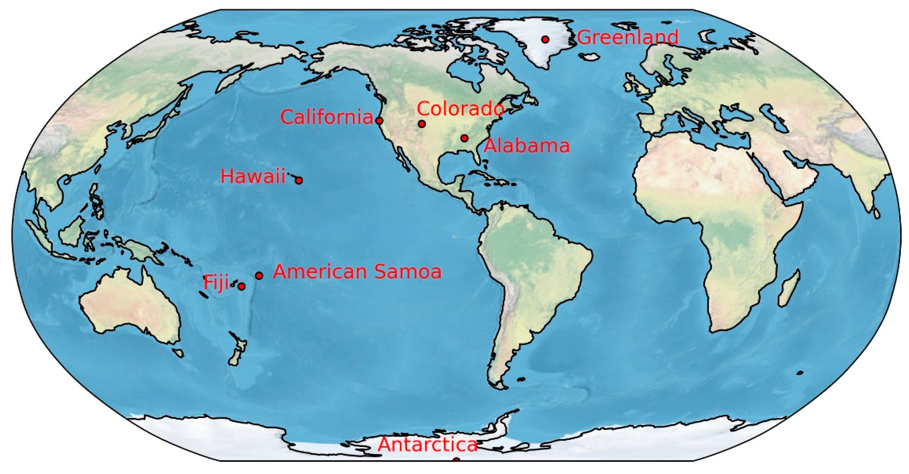
All the ozonesonde data used for this analysis were downloaded from NOAA ESRL’s ozonesondes website at https://gml.noaa.gov/ozwv/ozsondes/index.html (accessed on 9 June 2022). This archive includes data for 8 main weather stations that are distributed across the globe (but with the majority located in USA or its territories), that collectively cover the tropics, mid-latitudes and polar regions [12]—see Table 1. These locations are shown in Figure 1.

Table 1.
Details on the eight ozonesonde stations used in this analysis.

Figure 1.
Locations of the eight ozonesonde stations.
Some of these stations have longer records than others—in particular, both the Colorado and Antarctica archives include some low resolution sondes as early as 1967. However, some of the stations are relatively recent and several appear to have been discontinued in recent years. Additionally, the reliability, quality and resolution of the ozonesonde instruments has substantially improved in recent years [12]. Therefore, we have confined our analysis in this study to the year 2016, since all eight stations were active for this year and the data is of a very high quality. See Figure 1 of Sterling et al. (2018) for a graphical breakdown of the available data up to 2017 and the changes in instrumentation over time for each station [12].
The exact format of the data in the archive varies somewhat between stations and over time. However, in general, NOAA ESRL provide two main versions of the data:
- The raw native resolution files that for the 2016 sondes are reported roughly every second
- Interpolated “100 m average” versions that have been interpolated by NOAA ESRL from the raw data into smoother but lower resolution sondes.
Our analysis is based on the raw sondes.
As can be seen from Table 1, during 2016, ozonesondes were launched roughly once per week for most of the stations, although Fiji and American Samoa were less frequent. In total, 361 sondes were launched between these eight stations during 2016. However, in a few cases (5 out of 361, 1.4%), the sondes did not have sufficient data for analysis. Therefore, our analysis was based on 356 of the 361 sondes.
2.2. Methods
Each balloon provides in situ measurements approximately every second throughout their vertical ascent and descent in the troposphere, tropopause and stratosphere (up to ~30–35 km altitude) with readings of: altitude (h); pressure (P); temperature (T); water vapor (H2O); ozone (O3); horizontal wind speed and direction; and vertical ascent and descent velocity. For our analysis here, we will not be considering the horizontal wind measurements or vertical velocity measurements. However, we note that our preliminary analysis (not shown here) suggests that there might also be some systemic changes in these measurements associated with the troposphere/tropopause transition. We also note that the data from these sondes is sufficient to study the horizontal mass fluxes, as described by Connolly et al. (2021) [13].
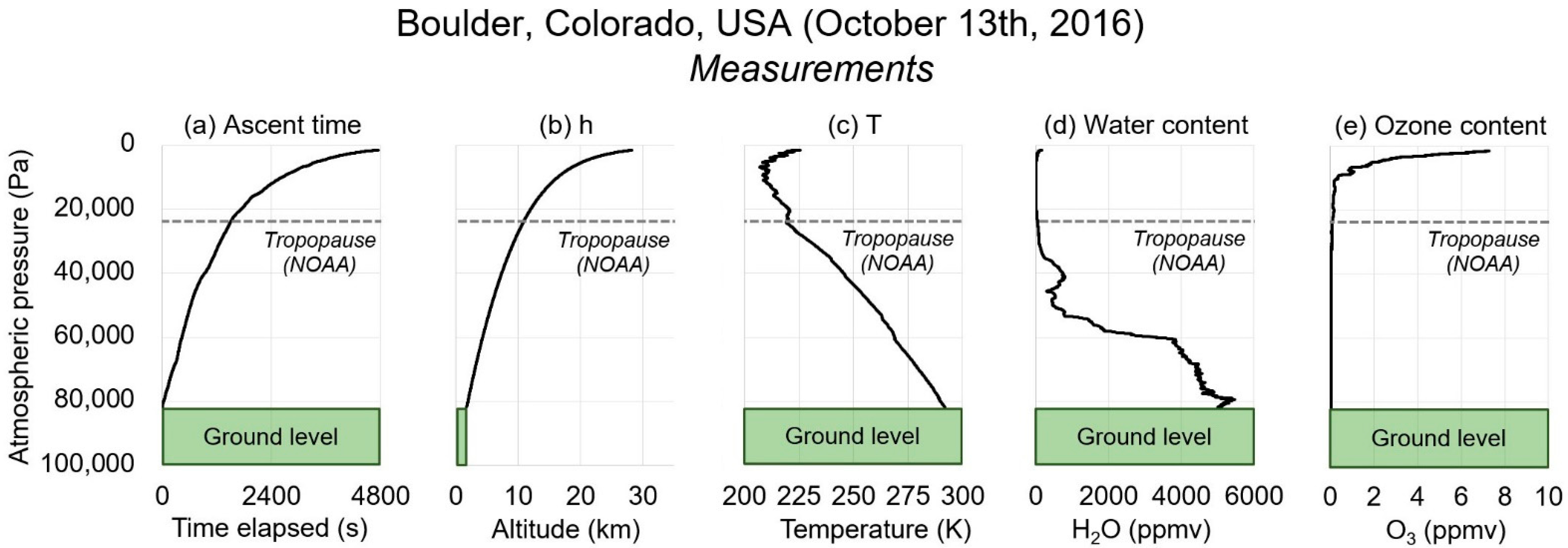
As a representative example, Figure 2 plots the relevant measurements for our analysis from one of the 356 ozonesondes launched from the Boulder, Colorado site–13 October 2016. NOAA provide with each sonde their calculated estimate of the tropopause height, which we have converted into the corresponding atmospheric pressure and indicated with horizontal dashed (gray) lines in each panel. We have not yet confirmed exactly how these values are calculated, however they appear to be derived by applying the WMO (1957)’s tropopause definition [2] to the temperature lapse rates of the interpolated data.
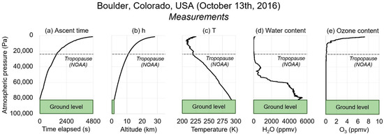
Figure 2.
Relevant measurements from a typical ozonesonde plotted against atmospheric pressure—launched from Boulder, Colorado on 13 October 2016. (a) Time elapsed since the sonde was launched; (b) altitude; (c) temperature; (d) water content; (e) ozone content. NOAA’s estimate of the tropopause (as provided with each ozonesonde record) is indicated in each panel by a horizontal dashed gray line. As Boulder is a mountainous location, the ground level has a relatively low atmospheric pressure as indicated by the green boxes in panels (a,c–e).
Figure 3 plots some of the relevant calculated measurements from Figure 2 that we use for our analysis. We determine the tropopause in four different ways:
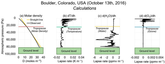
Figure 3.
Calculated metrics from the same ozonesonde as Figure 2. (a) The observed molar density is plotted in black along with a straight line slope in yellow that is fit over the region 30,000–50,000 Pa, as discussed in the text; (b) temperature lapse rate in K m−1; (c) water content lapse rate in ppmv m−1; (d) ozone content lapse rate in ppmv m−1. All lapse rates are calculated using a 31-point centered box car average. The tropopause calculated from each approach is indicated on the corresponding panel by horizontal dashed lines with distinct colors matching those in Figure 4.
- Molar density. The molar density, D, at each point is calculated from the corresponding pressure and temperature measurements, following the approach described by Connolly et al. (2021) [13]. That is, D = P/RT, where R = the ideal gas constant. To calculate the tropopause using molar density, we use two derived metrics: the rate of change of D with altitude, dD/dh; the rate of change of D with pressure, dD/dP. We also study the deviation of the observed D values from a linear fit in the upper troposphere region. This region is defined as 35,000–50,000 Pa for Greenland and Antarctica; 30,000–50,000 Pa for Colorado, Alabama; 25,000–45,000 Pa for California; 15,000–35,000 Pa for Hawai’i; 15,000–40,000 Pa for American Samoa and Fiji. We define the molar density-based tropopause as the pressure above the boundary layer at which:
- D significantly deviates from linearity—see Figure 3a for an example.
- dD/dh and dD/dP begin to oscillate wildly.
- Temperature. To calculate the tropopause from the temperature data, we calculate the rate of change of temperature with altitude, dT/dh; and with pressure, dT/dP. We define the temperature-based tropopause as the pressure above the boundary layer at which:
- dT/dh crosses from being negative to being positive.
- dT/dh and dT/dP begin to oscillate wildly—see Figure 3b for an example of this phenomenon for dT/dh.
- Water. To calculate the tropopause from the water vapor content data, we calculate the rate of change with altitude, d(H2O)/dh and with pressure, d(H2O)/dP. We define the water-based tropopause as the pressure above the boundary layer at which:
- [H2O] is less than 50 ppmv.
- d(H2O)/dh drops to zero.
- d(H2O)/dh and d(H2O)/dP stops oscillating wildly—see Figure 3c for an example for d(H2O)/dh.
- Ozone. To calculate the tropopause from the ozone content data, we calculate the rate of change with altitude, d(O3)/dh and with pressure, d(O3)/dP. We define the ozone-based tropopause as the pressure above the boundary layer at which:
- [O3] is greater than 0.1 ppmv.
- d(O3)/dh increases substantially and d(O3)/dP decreases substantially.
- d(O3)/dh and d(O3)/dP both begin to oscillate—see Figure 3d for an example for d(O3)/dh.
All rates of change calculations are calculated using a 31-point centered box car average, i.e., averaging over the ~15 s before and after a given measurement.
3. Results and Discussion
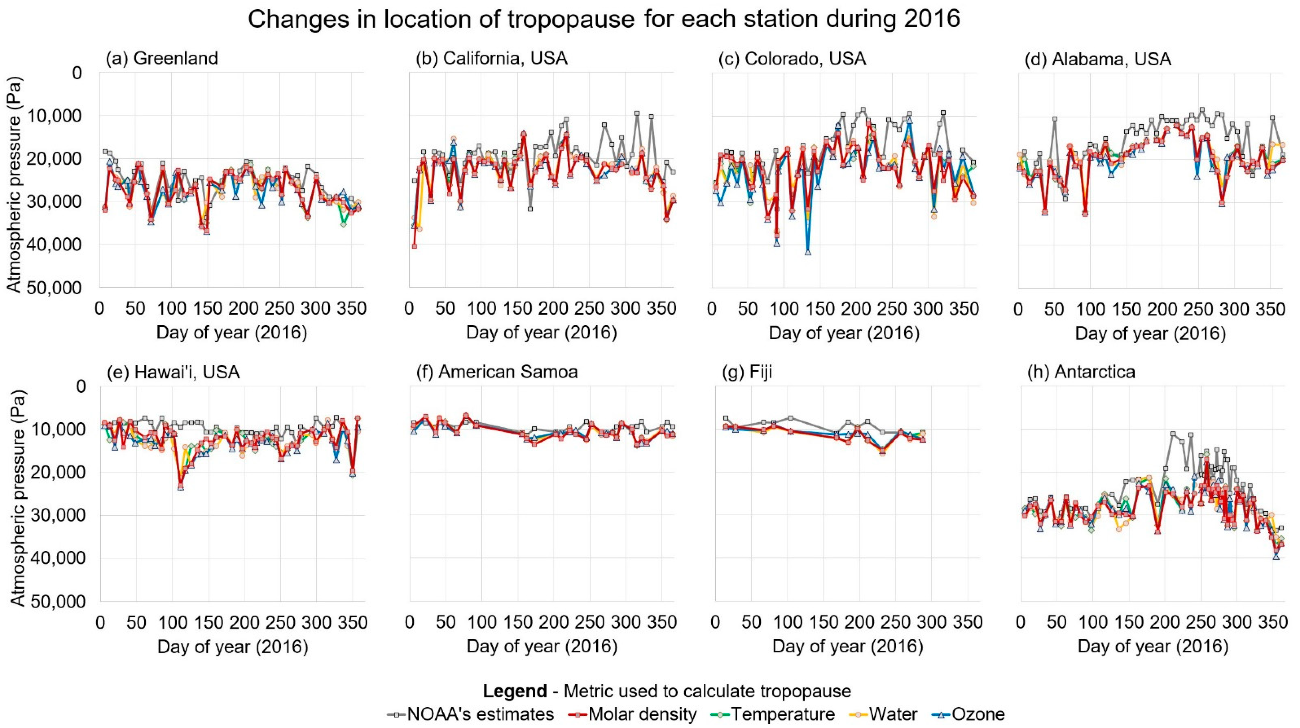
Figure 4 shows all five estimates of the tropopause for all 356 ozonesondes—sorted by day of year (in 2016) and station. We note that all five estimates match very well. However, NOAA’s estimates often seem to deviate from the other estimates. When this deviation occurs, it usually estimates a higher altitude than the other four. The deviation might have a seasonal factor in that it can last for several months, but the analysis in this study is confined to just one year, and the possibility of seasonality would need further research. A long-term analysis that combines the modern data with earlier sondes should probably take into account the various changes in instrumentation that have been adopted at each of the stations—see Sterling et al. (2018) for a summary [12].
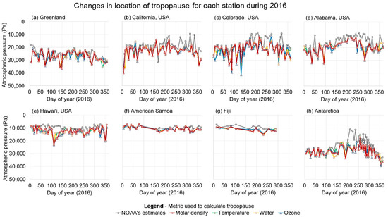
Figure 4.
Changes in the location of the tropopause for the eight stations for the entire year of 2016, as calculated using each of the metrics described in the text: (a) Greenland; (b) California, USA; (c) Colorado, USA; (d) Alabama, USA; (e) Hawai’i,USA; (f) American Samoa; (g) Fiji; (h) Antarctica. The colors used for each estimate are the same ones used for the equivalent horizontal lines in Figure 2 and Figure 3.
Table 2 statistically describes the high correlation between the four new estimates described here, and the moderate correlation with NOAA’s estimates.
Table 2.
Correlation coefficients (r, where 0 = uncorrelated, 1 = exactly correlated) comparing the tropopauses calculated by each approach to the other estimates over all ozonesondes launched in 2016 for each station. The averages for all eight stations are listed in the last column in the table.
We note that the WMO (1957)’s tropopause definition was formulated using much lower resolution weather balloon sondes than the analysis in this paper [2]. Therefore, while NOAA’s estimates are very useful for comparison with other datasets, we suggest that the four new estimates described in this paper that were developed specifically from this higher resolution dataset could be more precise and accurate in describing the troposphere/stratosphere transitions.
In particular, the original concept of the tropopause was a region where the temperatures remained fairly constant (“paused”). Yet, we note from the very high temporal resolution of this dataset compared with the earlier weather balloons that if anything, the temperature lapse rate becomes much more chaotic and variable in the tropopause and stratosphere regions. Whereas the average temperature lapse rate is fairly constant in these regions, the short-term oscillations are surprisingly large—see Figure 3b.
We also highlight the use of molar density as a particularly insightful metric for describing these transitions. We find the striking change in the slope of molar density versus pressure at the tropopause to be indicative of a major change in atmospheric behavior, e.g., see Figure 3a. The other tropopause definitions we considered also indicate various complex transitions that all broadly coincide with this change in slope. Therefore, we hypothesize that a better understanding of the reasons for this change in slope could provide a much deeper understanding of the many phenomena associated with the troposphere/stratosphere transitions. Two of the authors (MC & RC) have provided some hypotheses on this in a series of working papers in 2014 [14,15,16].
4. Conclusions
Since the turn of the 20th century, meteorologists have been fascinated by the striking contrasts between the lower atmosphere (troposphere) and the tropopause/stratosphere regions. Now, in the 21st century, we have access to increasingly high quality and high resolution weather balloon datasets, including ozonesondes. For this study, we used the very high quality ozonesonde archive of NOAA ESRL to study the troposphere/stratosphere transition, i.e., the tropopause.
This unique dataset allowed us to empirically compare and contrast five different definitions of the tropopause. We analyzed one complete year (2016) of ozonesonde data from the eight stations in the dataset that ranged from the tropics to the poles. These definitions appear to hold over all eight locations—from the tropics to the poles—for all seasons.
We found very high correlations between most of the definitions of the tropopause, although the correlations with the standard WMO (1957) definition were a bit lower. Contrary to the original concept of the tropopause being a region with very little temperature variability, the high temporal resolution of this dataset reveals that this only applies to the averages over large distances. Over shorter distances/time intervals, the temperature lapse rate varies quite wildly in the tropopause/stratosphere—especially when compared to the troposphere.
One of the tropopause definitions that we considered is based on molar density calculations. This provides an additional value to the molar density calculations which have been described previously by Connolly et al. (2021) [13].
Author Contributions
All authors contributed equally to this manuscript. Conceptualization, O.D., M.C., R.C. and W.S.; methodology, O.D., M.C., R.C. and W.S.; formal analysis, O.D., M.C., R.C. and W.S.; writing—original draft preparation, O.D., M.C., R.C. and W.S.; writing—review and editing, O.D., M.C., R.C. and W.S. All authors have read and agreed to the published version of the manuscript.
Funding
R.C. and W.S. received financial support from the Center for Environmental Research and Earth Sciences (CERES) while carrying out the research for this paper. The aim of CERES is to promote open-minded and independent scientific inquiry. For this reason, donors to CERES are strictly required not to attempt to influence either the research directions or the findings of CERES. Readers interested in supporting the work of CERES can donate at http://ceres-science.com/ (accessed on 9 June 2022).
Institutional Review Board Statement
Not applicable.
Informed Consent Statement
Not applicable.
Data Availability Statement
All the ozonesonde data used for this analysis were downloaded from NOAA Earth System Research Laboratories (ESRL)’s ozonesondes website at https://gml.noaa.gov/ozwv/ozsondes/index.html (accessed on 9 June 2022).
Conflicts of Interest
The authors declare no conflict of interest.
References
- Hoinka, K.P. The Tropopause: Discovery, Definition and Demarcation. Meteorol. Z. 1997, 6, 281–303. [Google Scholar] [CrossRef]
- WMO. Meteorology—A Three-Dimensional Science. WMO Bull. 1957, 6, 134–138. [Google Scholar]
- Reed, R.J. A study of a characteristic tpye of upper-level frontogenesis. J. Meteor. 1955, 12, 226–237. [Google Scholar] [CrossRef]
- Hoskins, B.J.; McIntyre, M.E.; Robertson, A.W. On the Use and Significance of Isentropic Potential Vorticity Maps. Q. J. R. Meteorol. Soc. 1985, 111, 877–946. [Google Scholar] [CrossRef]
- Holton, J.R.; Haynes, P.H.; McIntyre, M.E.; Douglass, A.R.; Rood, R.B.; Pfister, L. Stratosphere-Troposphere Exchange. Rev. Geophys. 1995, 33, 403–439. [Google Scholar] [CrossRef]
- Highwood, E.J.; Hoskins, B.J. The Tropical Tropopause. Q. J. R. Meteorol. Soc. 1998, 124, 1579–1604. [Google Scholar] [CrossRef]
- Zhou, X.L.; Geller, M.A.; Zhang, M.H. Tropical Cold Point Tropopause Characteristics Derived from ECMWF Reanalyses and Soundings. J. Climate 2001, 14, 1823–1838. [Google Scholar] [CrossRef]
- Gettelman, A.; Hoor, P.; Pan, L.L.; Randel, W.J.; Hegglin, M.I.; Birner, T. The Extratropical Upper Troposphere and Lower Stratosphere. Rev. Geophys. 2011, 49, RG3003. [Google Scholar] [CrossRef]
- Bethan, S.; Vaughan, G.; Reid, S.J. A Comparison of Ozone and Thermal Tropopause Heights and the Impact of Tropopause Definition on Quantifying the Ozone Content of the Troposphere. Q. J. R. Meteorol. Soc. 1996, 122, 929–944. [Google Scholar] [CrossRef]
- Folkins, I.; Loewenstein, M.; Podolske, J.; Oltmans, S.J.; Proffitt, M. A Barrier to Vertical Mixing at 14 Km in the Tropics: Evidence from Ozonesondes and Aircraft Measurements. J. Geophys. Res. Atmos. 1999, 104, 22095–22102. [Google Scholar] [CrossRef]
- Fischer, H.; Wienhold, F.G.; Hoor, P.; Bujok, O.; Schiller, C.; Siegmund, P.; Ambaum, M.; Scheeren, H.A.; Lelieveld, J. Tracer Correlations in the Northern High Latitude Lowermost Stratosphere: Influence of Cross-Tropopause Mass Exchange. Geophys. Res. Lett. 2000, 27, 97–100. [Google Scholar] [CrossRef]
- Sterling, C.W.; Johnson, B.J.; Oltmans, S.J.; Smit, H.G.J.; Jordan, A.F.; Cullis, P.D.; Hall, E.G.; Thompson, A.M.; Witte, J.C. Homogenizing and Estimating the Uncertainty in NOAA’s Long-Term Vertical Ozone Profile Records Measured with the Electrochemical Concentration Cell Ozonesonde. Atmos. Meas. Tech. 2018, 11, 3661–3687. [Google Scholar] [CrossRef]
- Connolly, M.; Connolly, R.; Soon, W.; Velasco Herrera, V.M.; Cionco, R.G.; Quaranta, N.E. Analyzing Atmospheric Circulation Patterns Using Mass Fluxes Calculated from Weather Balloon Measurements: North Atlantic Region as a Case Study. Atmosphere 2021, 12, 1439. [Google Scholar] [CrossRef]
- Connolly, M.; Connolly, R. The Physics of the Earth’s Atmosphere I. Phase Change Associated with Tropopause. Open Peer Rev. J. 2014, 19. Available online: http://oprj.net/articles/atmospheric-science/19 (accessed on 26 August 2022).
- Connolly, M.; Connolly, R. The Physics of the Earth’s Atmosphere II. Multimerization of Atmospheric Gases above the Troposphere. Open Peer Rev. J. 2014, 22. Available online: http://oprj.net/articles/atmospheric-science/22 (accessed on 26 August 2022).
- Connolly, M.; Connolly, R. The Physics of the Earth’s Atmosphere III. Pervective Power. Open Peer Rev. J. 2014, 25. Available online: http://oprj.net/articles/atmospheric-science/25 (accessed on 26 August 2022).

Publisher’s Note: MDPI stays neutral with regard to jurisdictional claims in published maps and institutional affiliations. |
© 2022 by the authors. Licensee MDPI, Basel, Switzerland. This article is an open access article distributed under the terms and conditions of the Creative Commons Attribution (CC BY) license (https://creativecommons.org/licenses/by/4.0/).