Proceeding Paper

Forecasting Monthly Rainfall of Karyes, Chios Island, Greece, Central-Eastern Mediterranean Basin Using the ARIMA Method †

by
Thomas Papalaskaris
Department of Civil Engineering, Democritus University of Thrace, Kimmeria Campus, 67100 Xanthi, Greece
Presented at the 4th EWaS International Conference: Valuing the Water, Carbon, Ecological Footprints of Human Activities, Online, 24–27 June 2020.
Environ. Sci. Proc. 2020, 2(1), 68; https://doi.org/10.3390/environsciproc2020002068
Published: 16 September 2020

Abstract

:
Chios Island undergoes scarcity of freshwater, forcing local authorities to establish a sea-water desalination plant to cope with island’s water needs. Karyes village is plentiful with freshwater springs, augmented every year by the rainfall occurring over this particular district, supplying, in turn, some high-quality freshwater obtaining spots into the capital of Chios, thus establishing an important freshwater origin of the entire Chios Island itself. The present study administers the Box–Jenkins method, utilizing SARIMA (Seasonal Autorregressive Integrated Moving Average) model to achieve short term predictions of monthly rainfall in Karyes village, modeling past rainfall time series and forecasting future ones. The model which best fits to both interpretations of the past rainfall data is selected, assessed by several statistical model evaluation criteria.

1. Introduction

Rainfall can be definitely considered as a non-linear natural process raising significant difficulties, especially while trying to forecast future values. Climate changes also provoke unfavorable conditions, worsening the problem causing the rainfall patterns to shift, sometimes quickly, from one state to another. Agricultural policy, crop engineering, tourism perspectives, flood protection civil works scheduling, rainwater harvesting strategy, urban water manipulation strategy, water storage reservoir capacity design, and a great number of other pluralistic activities related to water resource management are strongly influenced by both short-term as well as long-term rainfall predictions and forecasts. A variety of statistical procedures are often employed to forecast rainfall amounts. One of the mostly widespread methods for time series data analysis is that elaborated within the general context of stochastic hydrology [1], also bearing the name of SARIMA (Seasonal Autoregressive Integrated Moving Average). The SARIMA modeling technique has been applied worldwide on a great number of not only financial but, additionally, hydrological time series data in order to forecast rainfall data, water reservoir inflow/outflow discharge patterns, as well as river flows modeling [2]. Total monthly rainfall depth (mm) was forecasted, implementing Box–Jenkins method, for Kavala city, NE Aegean Sea, NE Greece, NE Mediterranean Basin [3,4]. A SARIMA model was developed to predict total monthly rainfall depth (mm), for Metaxades village area, Evros prefecture, NE Aegean Sea, NE Greece, NE Mediterranean Basin [5]. The Box–Jenkins method was also employed to build a SARIMA model and forecast total monthly rainfall depth (mm), for several streams in Eastern Macedonia-Thrace, NE Aegean Sea, NE Greece, NE Mediterranean Basin [6]. Another SARIMA was developed to predict total monthly rainfall depth (mm), for Karyes village area, Chios Island, NE Aegean Sea, NE Greece, NE Mediterranean Basin [7].

2. Methodology

2.1. Study Area

With the view of investigating rainfall patterns in the Karves countryside village area, located within the central sector (northeastern section) of Chios Island (six kilometers away from Chios’ main harbor), Northeastern Aegean Sea, Central-Eastern Mediterranean Basin, facing the Aegean Sea to the North and following an amphitreatical building construction pattern that provides a clear, distant, all-around observing view in all directions, total monthly recorded observations from the only available operating meteorological station, located at coordinates 683091 and 4250865 (EGSA’87 coordinates system) (altitude ~310 m), were analyzed, covering a time interval period of 37 years (February 1982–November 2018) as depicted in Figure 1.

2.2. The Box–Jenkins Model-Building Procedure

The statisticians Box and Jenkins (1970) developed a modeling method, primarily for financial time series analysis, dealing with stationary time series and fitting either autoregressive moving average (ARMA) or autoregressive integrated moving average (ARIMA) or seasonal autoregressive integrated moving average (SARIMA) models with the view to discover the most appropriate match of a time series data to previous values of the same time series, with the view to perform future predictions and forecasts. The model-building procedure incorporates the successive stages elaborated below [8].

2.2.1. Model Identification and Selection

Verifying the stationarity of the variables, tracing, and locating seasonality if it exists, within the time series data under investigation (a situation that can be treated by seasonal differencing) and interpreting charts of autocorrelation and partial autocorrelation functions of the time series data under examination with the view to conclude which autoregressive or moving average constituent would be the most appropriate to take place in the model.

2.2.2. Model Parameters Estimation

Calculations, in order to assay the most competent coefficients for the preferable ARIMA model, in most cases, were conducted by means of computation methods like either maximum likelihood estimation or least-squares estimation.

2.2.3. Model Checking and Forecasting

By examining whether the elaborated model complies with the requirements of a stationary univariate process, namely, the residuals should be independent between each other and exhibit constancy in terms of mean and variance along the entire length of the time series, as the time passes by. This can be carried out by plotting the mean and variance of residuals over time and executing a Ljung–Box test or/and charting autocorrelation and partial autocorrelation functions of the residuals as a means to verify whether the model we built best fit our time series data or not.

2.3. Types of ARIMA Models

2.3.1. Autoregressive (AR) and Moving Average (MA) Models

In an autoregression model, we forecast the variable of interest using a linear combination of past values of the variable. The term autoregression indicates that it is a regression of the variable against itself [4]. Thus an autoregressive model of order p can be written as:
y t = c + φ 1 × + × y t 2 + + φ p × y t p + e t
where c is a constant and et is white noise. This procedure resembles a multiple regression but with lagged values of yt as predictors. Reference is made to this type of model as an AR(p) model.

2.3.2. Autoregressive Moving Average (ARMA) Models

Instead of using past values of the forecast variable in a regression process, a moving average model uses past forecast errors within a regression-resembling model building [5]:
y t = c + e t + θ 1 × y t 1 + θ 2 × y t 2 + + θ q × y t q
where et is white noise. We make reference to this type of model as an MA(q) model.

2.3.3. Seasonal ARIMA (SARIMA) Models

ARIMA models possess also the ability to model seasonal data of a great extent. A seasonal ARIMA model, or so-called SARIMA model, is generated by incorporating supplementary seasonal components in the ARIMA models we have already mentioned above and it can be written in the following form [6]:
ARIMA (p,d,q,) (P,D,Q,)m
with p = non-seasonal (AR) order, d = non-seasonal differencing, q = non-seasonal (MA) order, P = seasonal (AR) order, D = seasonal differencing, Q = seasonal (MA) order, and where m = number of periods per season or, in other words, the time interval of repeating seasonal behavior. The seasonal components of the model are written by means of uppercase letters, whilst, on the contrary, we write the non-seasonal components of the model via lowercase letters. The seasonal portion of the model is comprised of components greatly resembling the non-seasonal terms of the model, yet they include backshift operators of the seasonal period. The additional seasonal components are multiplied through a simple method with the non-seasonal components of the model.

3. Results

3.1. Primordial Data Analysis

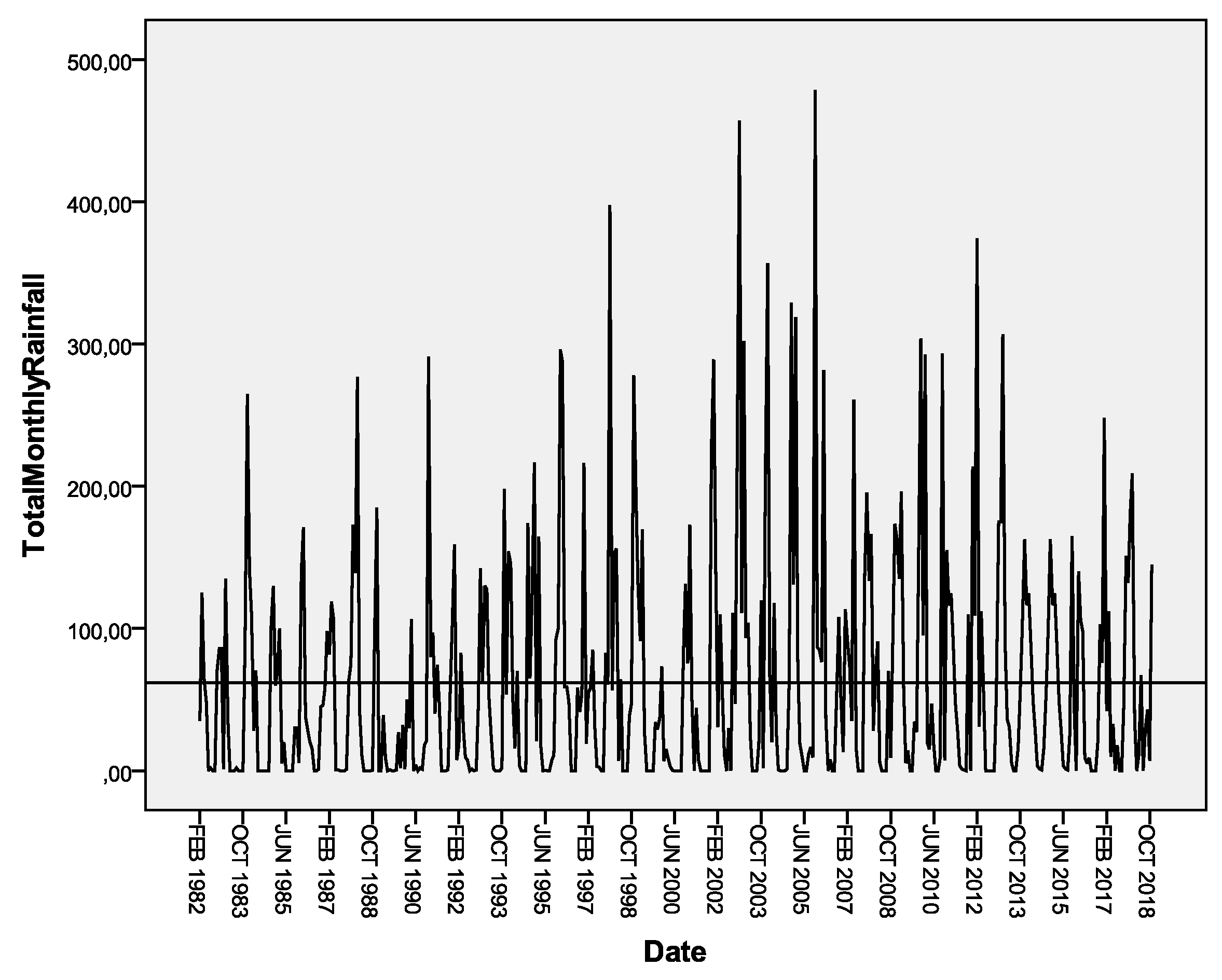
Primordial time series analysis was carried out dealing with total monthly rainfall data recorded from February 1982–November 2018 (37 years) employing the Box–Jenkins ARIMA model-building procedure. In the beginning a fairly simple time series chart was plotted using the unprocessed recorded data (total monthly rainfall data versus time/months) with the view to trace, by first sight, whether the mean or the variance of the time series either exhibits constancy over time or shifts as the time passes by, yielding Figure 2 [3,4,5,6,7].
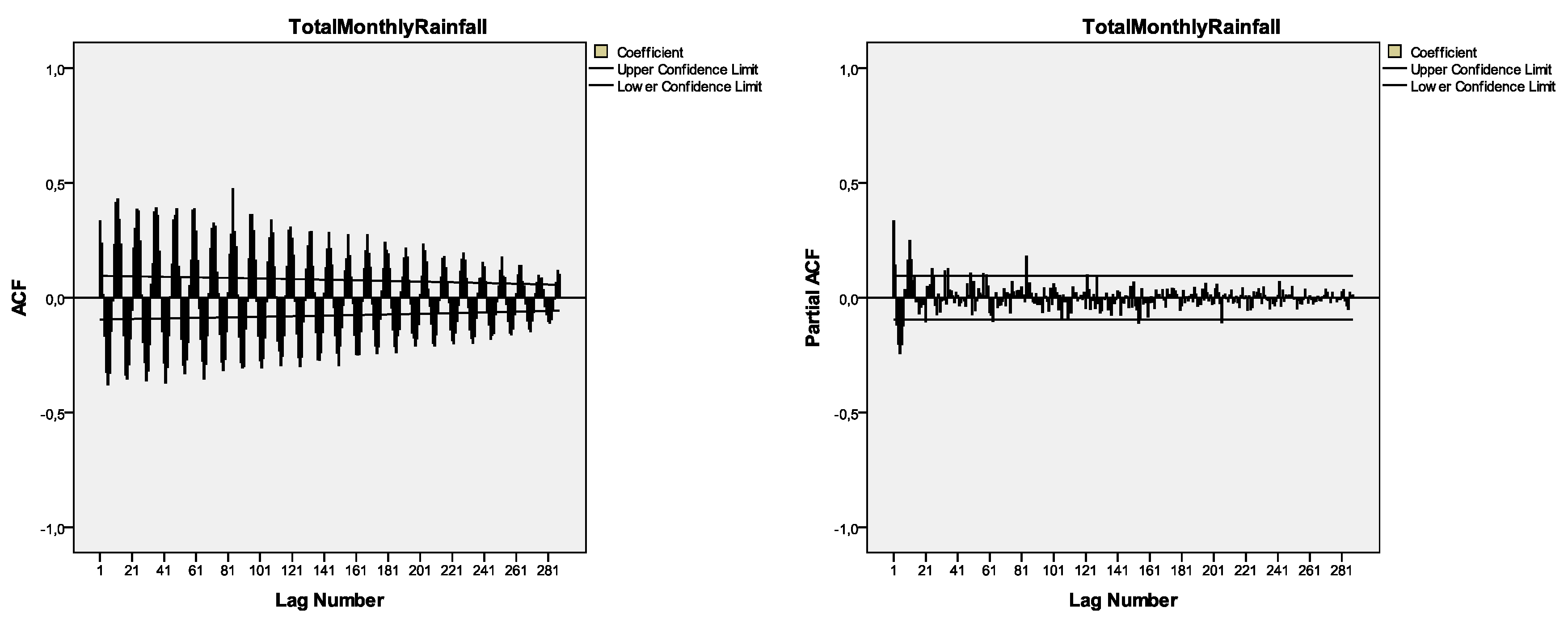
By first sight, the chart evidences that the time series seems to be stationary. By definition, a time series is considered non-stationary, when its values mean and variance either do not exhibit stability over time in terms of mean and variance. The ACF and PACF charts inspection can also provide clues of trend and seasonality existence. In order to better evaluate the ACF and PACF patterns, I selected to specify 288 autocorrelation lags concerning the total monthly rainfall data although Box and Jenkins’ (1970) suggestion was that the estimated autocorrelations number would be calculated for k = 0, 1, …, k, should not be larger in value than N/4, (444/4 = 111 regarding this particular case study), whilst their complementary suggestion that we would need at least 50 observations is also fulfilled since 444 > 50 [8]. The ACF and PACF charts examination shows evidences that seasonality trend exists which has to be eliminated with the view to achieve stationarity of the time series data. Seasonality often results to non-stationary time series owing to the fact that the average values along different parts of the time series occurring within the seasonal time interval differ from the average values along other segments of the same time series. A usual practical rule while interpreting an ACF chart is if there are designed autocorrelation bars that are larger in value than two standard errors apart from the zero mean, then they suggest proxy of autocorrelation which is statistically significant [3,4,5,6,7,8]. The ACF plot reveals alternative positive and negative values, decaying to zero, suggesting the use of an autoregressive model [8]. In Figure 3, there are several charted autocorrelation values, at different lags that either extend more (or close to) than two standard errors from the mean, represented by the zero value whilst the two continues lines designed above and below the zero mean stand for the approximate 95% confidence limits.
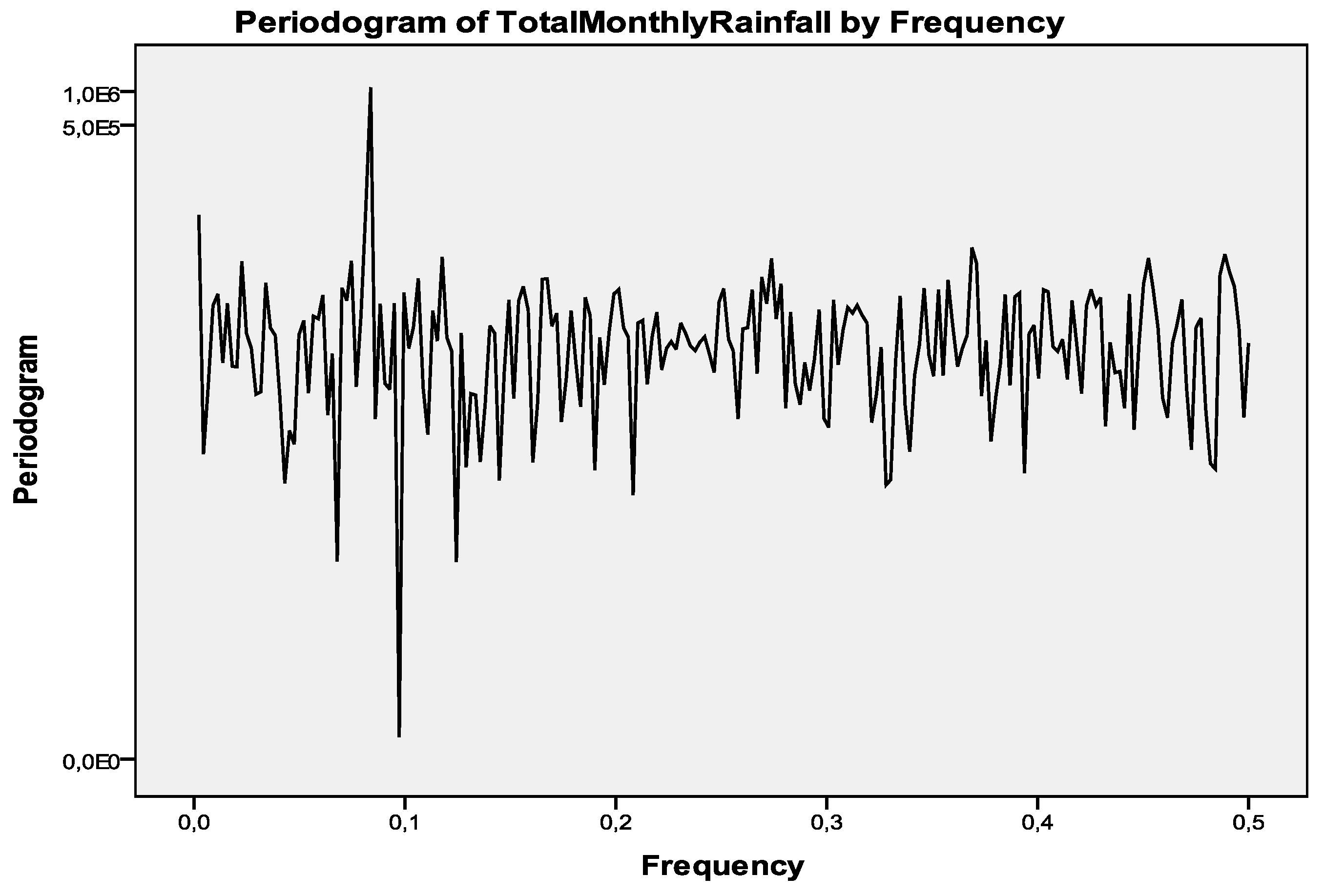
Visually inspecting, an anticipated conventional six-month seasonal pattern, following a cyclical pattern between the summer period during which the recorded rainfall levels are very low or zero and the winter period during which the rainfall reaches its highest levels, cannot be definitely either traced or recognized. Furthermore it should be noted that the performance of the time series analysis in the spectral domain, and after having examined the spectral density graph, proving that the largest seasonal pattern takes place at approximately 12 months’ time intervals, instead of six-month intervals [8]. Hence, we conclude that, by charting the ACF plot, the seasonality pattern unfolds, which could not be discovered by the simple linear equation describing the linear trend line associated with the original raw total monthly recorded rainfall data. This pattern can be easily identified in Figure 4 (left chart), focusing on the high peak at close a period of 12 months.

3.2. Data Stationarity Check

The Augmented Dickey-Fuller Unit Root Test, expressed within three different models, was employed and applied on the entire total monthly recorded rainfall time series data with the view to investigate and verify whether the rainfall time series is stationary or not. Table 1 depicts the outcomes of the test: In the first model (intercept only), the test statistic value −14.754 is lower in value than the critical values −3.445, −2.872, and −2.570, all at 1%, 5%, and 10%, correspondingly. Moreover, the regression coefficient L1 is negative in value (L1 = −0.6640124), hence, we can accept the model as a valid one. In the second model (trend and intercept), the test statistic value –14.879 is lower in value than the critical values −3.982, −3.422, and −3.130, all at 1%, 5%, and 10%, in consequence. Additionally, the regression coefficient L1 is once again negative in value (L1 = −0.6722652). Consequently, the model can be definitely considered as a valid one. In the third and last model (neither trend nor intercept), the test statistic value −10.832 is lower in value than the critical values −2.580, −1.950, and −1.620, all at 1%, 5%, and 10%, successively. Furthermore, the regression coefficient L1 is once again for this last model negative in value (L1 = −0.423204), therefore, the model can be definitely accepted as a valid one. Evidently, after having performed, examined, and checked all three different Augmented Dickey-Fuller Unit Root Tests we concluded in all cases that we reject the null hypothesis H0 and we accept the alternative hypothesis H1, which declares that the variable Y (total monthly recorded rainfall) is stationary and does not have a unit root [3,4,5,6,7].

3.3. Data Differencing (Seasonality)

Although the ADF test applied on the total recorded monthly time series of the raw data revealed it is a stationary time series, after examining the ACF chart depicted in the Figure 3, we considered that the time series data should be seasonally differenced, (due to a few spikes cut the 95% confidence limits), by order D = 1, in order to eliminate seasonality [3,4,5,6,7].

3.4. Model Identification

As soon as several tests concerning the total monthly recorded rainfall have been completed a few candidate models were considered that best meet the criteria and we finally concluded that the seasonal ARIMA (SARIMA) [(0,0,0) × (0,1,1)12] is considered the most suitable one appearing to have the least normalized Bayesian Information Criterion (B.I.C.) (8.394), Root Mean Squared Error (R.M.S.E.) (66.034), Mean Absolute Percentage Error (M.A.P.E.) (318.672), Mean Absolute Error (M.A.E.) (38.507), R-squared (0.364), and stationary R-squared (0.433) [3,4,5,6,7].

3.5. Model Adequacy and Diagnostic Tests

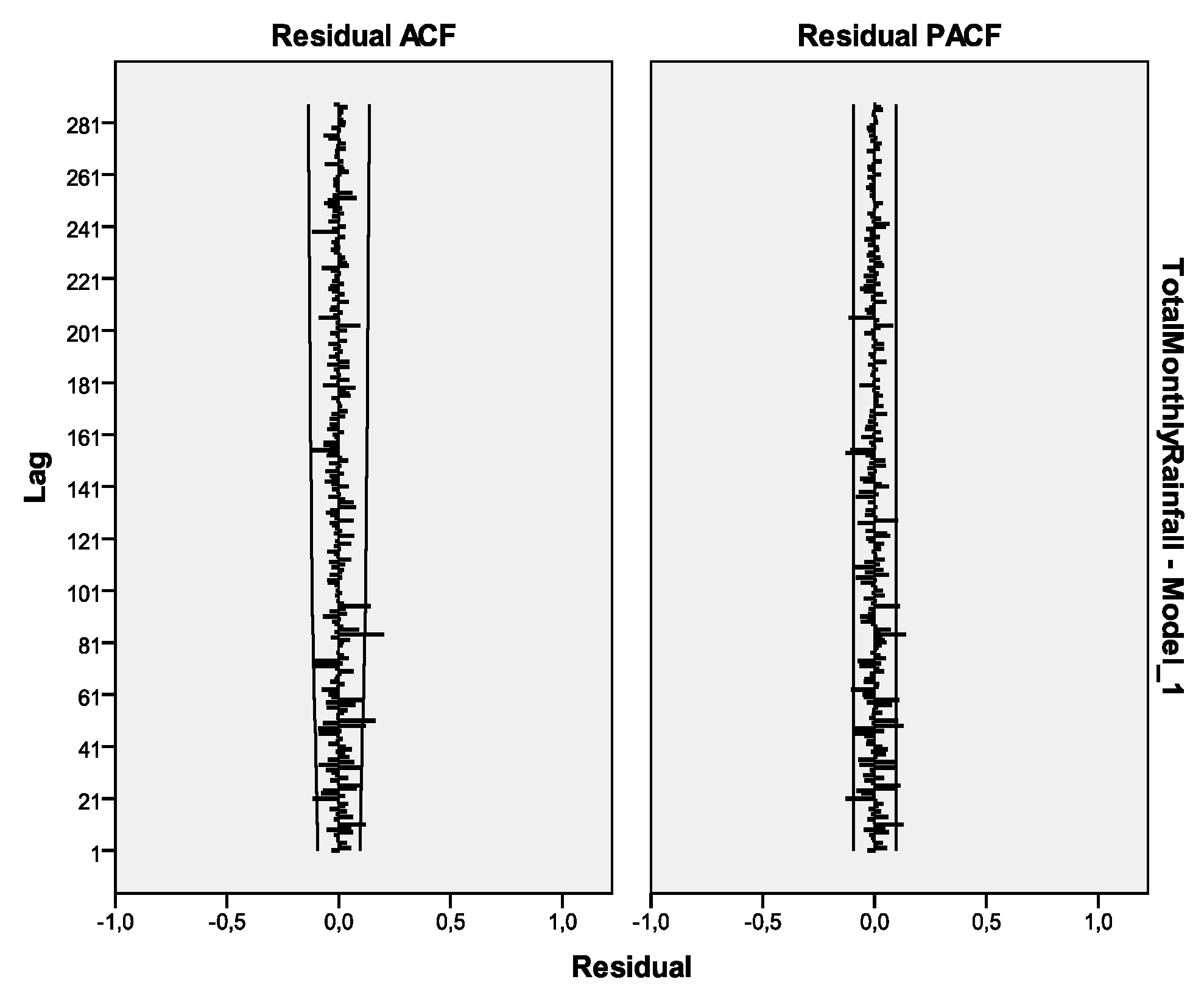
By examining in Figure 5 the autocorrelation and partial autocorrelation charts of the residuals we verify that there are only a few bar peak values that extend beyond the two continuous lines, plotted above and below the zero mean which imply the approximate 95% confidence limits [2,3,4,5,6,7].

3.6. Forecasting Future Values

Table 2 depicts the forecasted values.
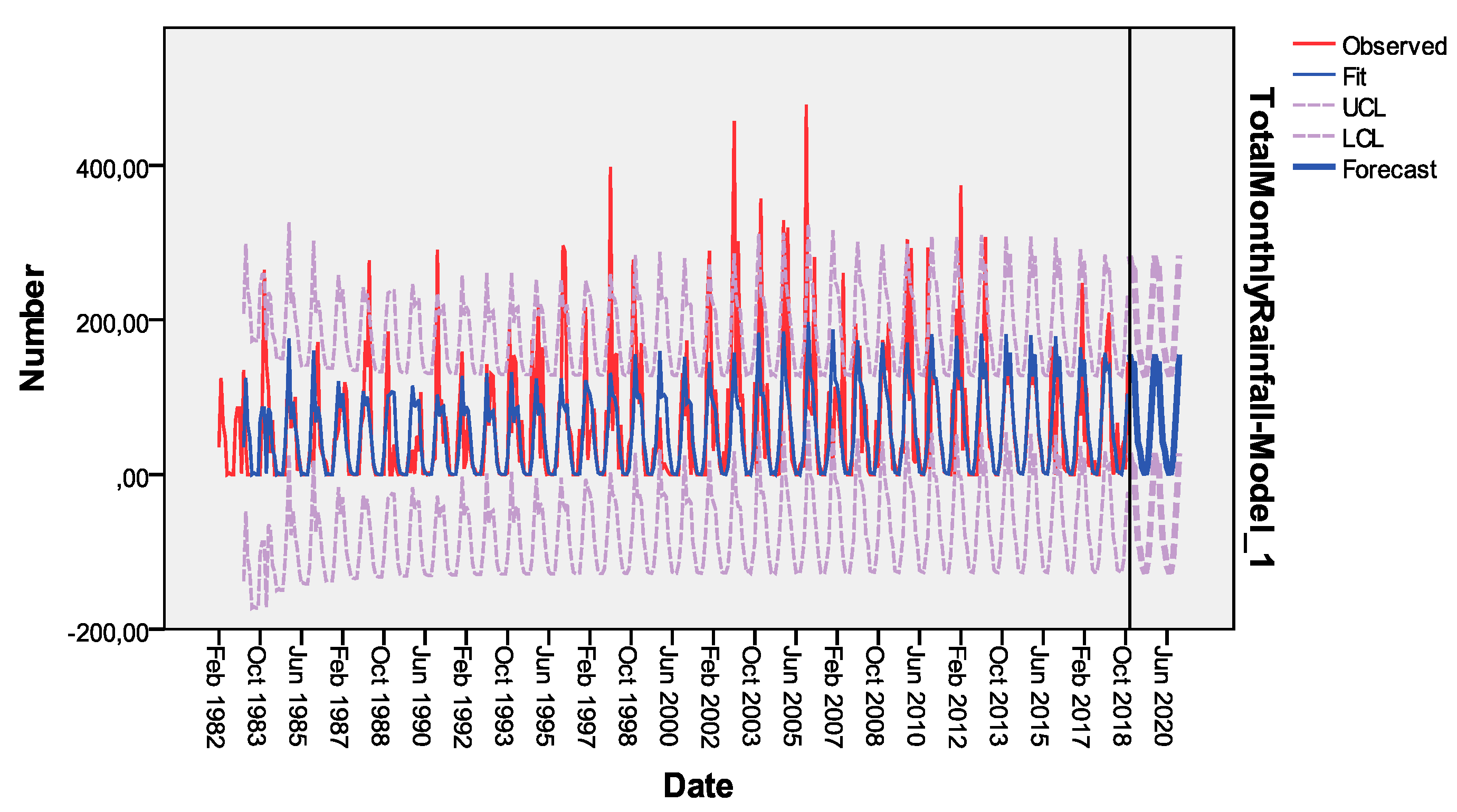
The observed, fit, and forecast values, as well as the upper and low confidence levels with reference to the finally selected SARIMA [(0,0,0) × (0,1,1)12] model, are all summarized within the chart illustrated by Figure 6 [3,4,5,6,7].

4. Conclusions

After having examined a group of candidate SARIMA models we concluded that the SARIMA [(0,0,0) × (0,1,1)12] model best fits the total recorded monthly rainfall data of the village countryside area of Karyes (central sector and northeastern section of Chios Island), Chios Island, Northeastern Aegean Sea, Central-Eastern Mediterranean Sea, Central-Eastern Mediterranean Basin, Greece, for the period February 1982–November 2018 (37 years). Still, it showed poor performance to capture high rainfall depths, suggesting that an ANN model, considering several meteorological parameters as inputs and rainfall depth as the output, might better simulate the higher forecasted values.

Author Contributions

All authors have read and agree to the published version of the manuscript.

Funding

This research received no external funding.

Acknowledgments

The author wishes to express that they feel grateful to Simeon Karaolanis, an Agronomist working for the Department of Plants and Animals production—Administration of Agricultural and Veterinary Economy, Chios Island Regional Unity—General Administration of Agricultural and Veterinary Economy, Regional Administration of North Aegean, Greece, who kindly supplied me the raw recorded and filed total monthly rainfall data of the village countryside area of Karyes, (central sector and northeastern section of Chios Island), Chios Island, Northeastern Aegean Sea, Central-Eastern Mediterranean Sea, Central-Eastern Mediterranean Basin, Greece.

Conflicts of Interest

The authors declare no conflict of interest.

References

  1. Abdul-Aziz, A.R.; Anokye, M.; Kwame, A.; Munyakazi, L.; Nsowah-Nuamah, N.N.N. Modeling and forecasting rainfall pattern in ghana as a seasonal arima process: The case of ashanti region. Int. J. Humanit. Soc. Sci. 2013, 3, 224–233. Available online: https://www.researchgate.net/publication/306940437_Modeling_and_forecasting_rainfall_pattern_in_Ghana_as_a_seasonal_ARIMA_process_The_case_of_Ashanti_region (accessed on 3 March 2020).
  2. Bari, S.H.; Rahman, M.T.; Hussain, M.M.; Ray, S. Forecasting monthly precipitation in sylhet city using ARIMA model. Civ. Environ. Res. 2015, 7, 69–77. Available online: https://www.researchgate.net/publication/272744442_Forecasting_Monthly_Precipitation_in_Sylhet_City_Using_ARIMA_Model (accessed on 3 March 2020).
  3. Papalaskaris, T.; Panagiotidis, T.; Pantrakis, A. Stochastic monthly rainfall time series analysis, modeling and forecasting in Kavala city, Greece, North-Eastern Mediterranean basin. In Proceedings of the 2nd Efficient & Sustainable Water Systems Management toward Worth Living Development 2016 (2nd “E.W.a.S.” 2016), Platanias-Chania-Crete Island, Greece, 1–4 June 2016; Kanakoudis, V., Karatzas, G.P., Keramaris, E., Eds.; University of Thessaly: Volos, Greece; Technical University of Crete: Crete, Greece, 2016. [Google Scholar]
  4. Papalaskaris, T.; Panagiotidis, T.; Pantrakis, A. Stochastic monthly rainfall time series analysis, modeling and forecasting in Kavala city, Greece, North-Eastern Mediterranean basin. Procedia Eng. 2016, 162, 254–263. [Google Scholar] [CrossRef]
  5. Papalaskaris, T.; Panagiotidis, T. Stochastic monthly rainfall time series analysis, modeling and forecasting in Metaxades area, Evros, Greece, North-Eastern Mediterranean basin. In Proceedings of the 3rd Greek Conference of Civil Protection (“Employing New Technologies for Civil Protection Purposes”) 2016 (3rd “Safe Evros” 2016), Alexandroupoli (Evros prefecture), Greece, 22–25 June 2016; Maris, F.P., Ed.; Prefecture of Eastern Macedonia & Thrace, Democritus University of Thrace: Alexandroupolis, Greece, 2016; pp. 443–452. [Google Scholar]
  6. Papalaskaris, T.; Kampas, G. Time series analysis of water characteristics of streams in Eastern Macedonia-Thrace, Greece. Eur. Water 2017, 57, 93–100. Available online: https://www.ewra.net/ew/pdf/EW_2017_57_13.pdf (accessed on 3 March 2020).
  7. Papalaskaris, T.; Panagiotidis, T. Stochastic monthly rainfall time series analysis, modeling and forecasting in Karyes, Chios Island, Greece, Central-Eastern Mediterranean Basin. In Proceedings of the 15th International Conference on Environmental Sscience & Technology 2017 (15th “C.E.S.T.” 2017), Rhodes Island, Greece, 31 August–2 September 2017; Lekkas, D.F., Klontza, E., Vrentzou, K., Eds.; University of the Aegean: Mytilene Island, Greece ID 01008. [Google Scholar]
  8. Box, G.E.P.; Jenkins, G.M.; Reinsel, G.C.; Ljung, G.M. Time Series Analysis: Forecasting & Control, Revised 5th ed.; John Wiley & Sons, Inc.: Hoboken, New Jersey, USA, 2015. [Google Scholar]
Figure 1. Map of the district of Karyes village, Chios Island, Northeastern Aegean Sea, Central-Eastern Greece (created using Google Earth and miscellaneous mapping).
Environsciproc 02 00068 g001
Figure 2. Total (recorded) monthly rainfall time series plot of the district of Karyes village, Chios Island, Northeastern Aegean Sea, Central-Eastern Greece.
Environsciproc 02 00068 g002
Figure 3. ACF and PACF charts of the total (recorded) monthly rainfall time series data of Karyes village district, Chios Island, Northeastern Aegean Sea, Central-Eastern Greece.
Environsciproc 02 00068 g003
Figure 4. Spectral density chart of the total (recorded) monthly rainfall time series data of Karyes village district, Chios Island, Northeastern Aegean Sea, Central-Eastern Greece.
Environsciproc 02 00068 g004
Figure 5. ACF and PACF charts of SARIMA [(0,0,0) × (0,1,1)12] model residuals of Karyes village district, Chios Island, Northeastern Aegean Sea, Central-Eastern Greece.
Environsciproc 02 00068 g005
Figure 6. Forecast chart of SARIMA [(0,0,0) × (0,1,1)12] model of Karyes village district, Chios Island, Northeastern Aegean Sea, Central-Eastern Greece.
Environsciproc 02 00068 g006
Table 1. ADF test on the raw total (recorded) monthly rainfall time series data (intercept only) of Karyes village district, Chios Island, Northeastern Aegean Sea, Central-Eastern Greece.
ADF Unit Root TestNumber of ObservationsTest StatisticInterpolated Dickey-FullerCoefficients
Test Statistic (1% Critical Value)Test Statistic (5% Critical Value)Test Statistic (10% Critical Value)L1_cons
Values444−14.754−3.445−2.872−2.570−0.664012441.09186
Table 2. Forecasted total monthly rainfall values of SARIMA [(0,0,0) × (0,1,1)12] model of Karyes village district, Chios Island, Northeastern Aegean Sea, Central-Eastern Greece.
SARIMA
Model
Dec
2018
Jan
2019
Feb
2019
Mar
2019
Apr
2019
May
2019
Jun
2019
Jul
2019
Aug
2019
Sep
2019
Oct
2019
Nov
2019
Forecast155.02140.41145.6787.1541.6130.319.242.262.8018.0761.07107.78
Publisher’s Note: MDPI stays neutral with regard to jurisdictional claims in published maps and institutional affiliations.