Abstract
This study investigates the backflow of a Newtonian fluid in a two-dimensional flat-walled fracture with Navier slip boundary conditions. The fracture has a uniform aperture and two rigid pre-strained plates as walls; their elastic deformations are described by the Winkler model. Under the lubrication assumption, the governing nonlinear ordinary differential equation and the time-dependent velocity profile are derived; in turn, this yields the time and space evolution of the pressure distribution inside the fracture, numerically. In addition, the condition when the external pressure becomes zero, is discussed, and a parametric study is performed to highlight the influence of the slip length.
1. Introduction
Backflow technology, known and in use for almost a century, has been revived and applied in recent decades to increase the production of gas and oil from shales, with further applications in the carbon sequestration and geothermal plants, see [1] for a review. The objective is to increase permeability by generating a network of fractures [2], which are then stabilised with proppant, usually sand particles, although in some applications an increased roughness of the fractures is sufficient to prevent closure after the backflow. The transport of the proppant requires adequate fluid characteristics; the fluid must be able to keep the particles in suspension while maintaining a reasonably low viscosity. Following the completion of the fracturing and proppant injection phases, it is necessary to recover the carrier fluid that is pumped out by both the elastic reaction of the fracture walls and the hydrocarbon advancement, see [3].
The dynamics are controlled by the elastic reaction of the fractured mass and the fluid rheology, as well as the geometry of single fractures and network. The fluid is almost always non-Newtonian, with a behaviour that can be described by different models with temperature-dependent characteristics. Fracking and proppant carrier fluids are, in fact, the subject of careful studies to ensure that their in situ behaviour satisfies the following requirements: (i) injectability without excessive resistance; (ii) ability to transport proppant particles; (iii) easy evacuation and backflow; (iv) protection of plants and environment.
The complexity of the process limits the effectiveness of the global models and has traditionally favoured the development of simple models capable of reproducing the basic processes, starting with the backflow, in a conceptual frame and in the laboratory [4,5,6], in plane or radial geometry, with Newtonian or non-Newtonian fluids.
In addition to the early contributions by Garagash [7], followed by several others (see the review by Osiptov [3]), we also mention other contributions [8,9,10,11], in which the fluids modelled with power-law or Ellis rheology, flow in fractures with a plane or radial symmetry.
It is a fact of evidence that many fluids do not meet the wall adhesion condition and are subject to slip; see Neto et al. [12] for a review of the experimental studies, and Lauda et al. [13] for a review of the theoretical approaches. The presence of a slip at the wall modifies the flow rate for a given pressure gradient and introduces further complexities to the scenario, even though the random geometry of the fracture has been left apart. For example, for a fracture surface wetted with creosote in a fracture half a millimeter wide, the increase in the flow rate was 10.0% compared to a surface wetted with water [14]. The change in the flow rate, however, seems to insignificantly influence the longitudinal dispersion rate [15].
The aim of the present paper is to analyse the backflow of a Newtonian fluid with a slip in an elastic fracture. The paper is organised as follows. Section 2 formulates the theoretical model and illustrates the approximations made. Section 3 describes the numerical model used for the integration of the resulting differential problem. Finally, the main results are summarised in the conclusions.
2. Theory
We consider a two-dimensional fracture with the finite length , time-dependent aperture , with an initial thickness of , filled with an incompressible fluid with a dynamic viscosity μ, as shown schematically in Figure 1. The fracture is characterised by two rigid plates having a flexural stiffness [5,16] yielding a constant aperture throughout the fracture length. At the initial time instant (), the fracture walls are subjected to a no-flow condition at the fracture inlet () and the constant initial pressure () at its outlet (). When time evolves () and the pre-strained upper plate is released, the fluid is squeezed out of the outlet; as a result, the direction of the pressure gradient inside the fracture is in the x-direction, resulting in a parabolic velocity profile towards the outlet. We denote and as the velocity field and pressure inside the fracture, respectively.
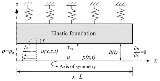
Figure 1.
The schematics of a two-dimensional fracture with a finite length L and an initial aperture
. Half of the fracture is shown due to the symmetry.
The incompressible flow is governed by the continuity equation
and the momentum equation in a coordinate free form reads
where is the fluid density, p the pressure including the gravity effects, u the velocity vector, and the deviatoric stress tensor. Considering an incompressible, steady, and laminar flow propagating in the x-direction (no movement in the z-direction), the momentum equation in the Cartesian system of Figure 1 becomes
Integrating the momentum Equation (3) for a constant viscosity fluid, one can obtain the relevant shear stress component as
where and c is a constant. The velocity of the fluid is obtained by integrating the momentum Equation (3) twice yielding
where and are two unknown real constants that can be obtained by imposing the boundary condition at the wall and the symmetry of the velocity profile for a pure Poiseuille flow ( for ) as
Substituting Equation (6) into Equation (5), the velocity profile for the half-fracture takes the form
2.1. Linear Navier Slip Law
We consider slip walls at the top and bottom plates constituted by the linear Navier slip law [5] where the relationship between the slip velocity us and shear stress is linear:
In Equation (8), is the slip length with the dimension [L]. Substituting Equation (4) into (8), the slip velocity for the walls () reads
We impose a flow rate for the inverse problem, where is the mean velocity across the channel calculated as
By integrating Equation (10) and substituting Equation (9) into Equation (6), the averaged velocity is obtained as
2.2. Governing Equations
We assume that the fracture aperture is much smaller than its length () and the lubrication assumption holds for the fluid confined between the plates. The one-dimensional continuity equation is obtained from the generalised Equation (1) as
Substituting Equation (11) into (12), we obtain a nonlinear equation for the fracture aperture in the form of
We exploit the Winkler model [17] to account for the elastic squeezing force exerted by the plates, where the plates are assumed to be stiff, and their deformations are independent of x. The Winkler support is envisioned as a cascade of elastic springs with a total effective elastic modulus of , where is the modulus of the elasticity of the beam and the initial thickness of the elastic springs; for an array of parallel fractures, equals the fracture spacing [10], see Figure 2.
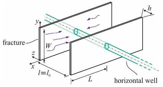
Figure 2.
Wing symmetric fractures with the spacing l. The blue arrows in the figure demonstrate the fluid flow.
When the pre-strained plates are released (), the reaction forces exerted from the springs to the plates are counterbalanced by the pressure developed in the fluid; hence, the force balance can be derived as
The initial and boundary conditions (BCs) of the problem are
2.2.1. Dimensionless Governing Equations
We define a set of dimensionless parameters as
The governing nonlinear Equation (13) and dynamic boundary condition in Equation (15) become
where is the dimensionless slip coefficient (or slip number) and the dimensionless external pressure. Subsequently, the initial condition and BCs of Equations (15) and (16) become
2.2.2. Nonlinear Ordinary Differential Equation (ODE)
We solve the dimensionless nonlinear Equation (18) subject to the initial and boundary conditions of Equations (20) and (21). From Equation (18), one can conclude that
where is an auxiliary function. Thus, Equation (18) can be rewritten as
We solve Equation (18) by applying the BCs of Equation (21),
The governing nonlinear ODE is obtained by substituting Equations (22) and (24) into Equation (19) as
We note that for the case of the no-slip condition, by assuming , we exactly recover the results of Dana et al. [5].
3. Numerical Results
We seek the numerical solution of Equation (25) by exploiting MATLAB subroutine ‘ODE45’ to solve the nonlinear first-order ODE, subjected to the initial condition of Equation (20). Figure 3 shows the numerical solutions obtained for five values of dimensionless pressure , and a slip number of obtained from the data included in the experimental study of Zheng et al. [15]. While the numerical result of the singular limit scenario tends to zero with a slope of in log-log scale, the late-time solutions () of asymptotically approach a constant value . We derive the analytical solution for the specific case (see Appendix A) to validate our numerical findings. The implicit Equation (A3) is solved by MATLAB subroutine ‘fsolve’ and super-imposed to Figure 3, where a good agreement between the semi-analytical (red circles) and numerical results (black line) are obtained. We note that the value is a limit for the borehole pressure.
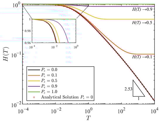
Figure 3.
Numerical solutions of the governing ODE of Equation (25) for the different values of Pe. The analytical result of the case Pe = 0 obtained from Equation (A3) is highlighted by the red dots.
The dimensionless time evolution and space of the pressure inside the fracture with no external pressure, is obtained from Equation (24) and shown in Figure 4. The pressure profiles are calculated for , respectively. It is evident that when time evolves, the pressure profiles flatten, and the pressure at the crack tip () decreases.
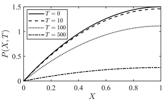
Figure 4.
Time evolution of the dimensionless pressure distribution of Equation (24) inside the fracture when the pressure gradient is null (Pe = 0).
Finally, we perform a parametric study on the effect of the slip length variation, considering just the case where the external pressure is zero (). We consider three values of in the order of based on the values obtained experimentally [10]. Figure 5 depicts the numerical solution of the nonlinear ODE for different slip numbers. The variation of the slip length does not substantially modify the overall behaviour of while the no-slip condition () is approaching zero with the largest slope, since no friction exists between the fluid and the fracture walls in this scenario.
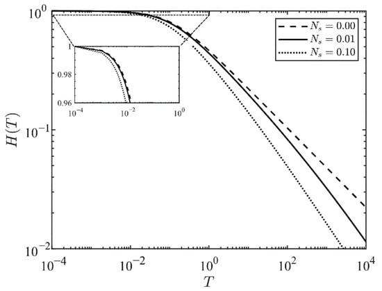
Figure 5.
Numerical solution of the ODE for the different Ns when the external pressure is null (Pe = 0).
4. Conclusions
Hydraulic fracturing has been widely investigated in recent years concerning the environmental effects caused by the release of by-products and fluid wastewater during the process of the hydrocarbons production from the fractured wells. The wastewater, also known as backflow, is generated from the relaxation of fracture elastic boundaries from a pre-strained state, counterbalanced by the internal pressure of the viscous fluid.
In this study, we investigated the backflow of a Newtonian fluid confined in a two-dimensional flat-walled fracture of length and a time-dependent aperture with an initial gap opening . The fracture is filled with an incompressible and viscous fluid; initially (), the fracture walls are subject to a no-flow condition at the far end of the fracture () and to the constant initial pressure () at its outlet (). When the pre-strained upper plate is released, the fluid is squeezed out of the outlet, and the fluid moves inside the fracture towards the outlet. The lubrication approximation applies to the confined fluid since the fracture aperture is assumed to be much smaller than its characteristic length. The linear Navier slip law, where the slip velocity varies linearly to the tangential stress, is applied as a boundary condition at the bottom and top plates. In addition, the Winkler model is exploited to determine the elastic deformation of the loaded plates.
Under these assumptions, the time evolution of the fracture aperture is obtained numerically by solving the governing dimensionless ODE for different external pressure values. The numerical result for the case is validated against a semi-analytical solution, and the effect of the slip length variation is investigated through a parametric analysis. For , the numerical solution tends to a constant value equal to the external pressure. Overall, this work provides new insights for the backflow analysis of fracturing liquids, and it can find numerous applications in civil, petrochemical, and environmental engineering.
Author Contributions
Conceptualization, F.Z. and V.D.F.; methodology, F.Z., A.L., S.L. and V.D.F. software, F.Z.; validation, A.L., S.L. and V.D.F.; writing—original draft preparation, F.Z., S.L. and V.D.F.; writing—review and editing, F.Z., A.L., S.L. and V.D.F.; visualization, F.Z.; supervision, S.L. and V.D.F.; project administration, V.D.F.; funding acquisition, V.D.F. All authors have read and agreed to the published version of the manuscript.
Funding
This research received no external funding.
Institutional Review Board Statement
Not applicable.
Informed Consent Statement
Not applicable.
Data Availability Statement
The data presented in this study are available upon request, from the corresponding author.
Acknowledgments
V.D.F. acknowledges the financial support from “Università di Bologna Ricerca Fondamentale Orientata (RFO) 2020” funds.
Conflicts of Interest
The authors declare no conflict of interest.
Appendix A
We look for the solution of the nonlinear first-order ODE of Equation (25) when the external pressure is null (). Following some rearrangements, Equation (25) becomes a separable differential equation and can be integrated as
which has a general solution
The unknown constant is which satisfies the initial condition of Equation (20). Hence the solution for the ODE in the case of
yields an implicit equation for in the form of
References
- Montgomery, C.; Smith, M. Hydraulic fracturing: History of an enduring technology. J. Pet. Technol. 2010, 62, 26–32. [Google Scholar] [CrossRef]
- Britt, L. Fracture stimulation fundamentals. J. Nat. Gas. Sci. Eng. 2012, 8, 34–51. [Google Scholar] [CrossRef]
- Osiptov, A. Fluid mechanics of hydraulic fracturing: A review. J. Pet. Sci. Eng. 2017, 156, 513–535. [Google Scholar] [CrossRef]
- Lai, C.-Y.; Zheng, Z.; Dressaire, E.; Ramon, G.; Huppert, H.E.; Stone, H. Elastic relaxation of fluid-driven cracks and the resulting backflow. Phys. Rev. Lett. 2016, 15, 24–36. [Google Scholar] [CrossRef] [PubMed]
- Dana, A.; Zheng, Z.; Peng, G.G.; Stone, H.A.; Huppert, H.E.; Ramon, G.Z. Dynamics of viscous backflow from a model fracture network. J. Fluid Mech. 2018, 836, 828–849. [Google Scholar] [CrossRef]
- McLennan, J.; Walton, I.; Moore, J.; Brinton, D.; Lund, J. Proppant backflow: Mechanical and flow considerations. Geothermics 2015, 57, 224–237. [Google Scholar] [CrossRef]
- Garagash, D.I. Transient solution for a plane-strain fracture driven by a shear thinning, power-law fluid. Int. J. Numer. Anal. Meth. Geomech. 2006, 30, 1439–1475. [Google Scholar] [CrossRef]
- Chiapponi, L.; Ciriello, V.; Longo, S.; Di Federico, V. Non-Newtonian backflow in an elastic fracture. Water Resour. Res. 2019, 55, 10144–10158. [Google Scholar] [CrossRef]
- Ciriello, V.; Lenci, A.; Longo, S.; Di Federico, V. Relaxation-induced flow in a smooth fracture for Ellis rheology. Adv. Water Resour. 2021, 152, 103914. [Google Scholar] [CrossRef]
- Lenci, A.; Chiapponi, L.; Longo, S.; Di Federico, V. Experimental investigation on backflow of power-law fluids in planar fractures. Phys. Fluids 2021, 33, 083111. [Google Scholar] [CrossRef]
- Zeighami, F.; Lenci, A.; Di Federico, V. Drainage of power-law fluids from fractured or porous finite domains. J. Non-Newton. Fluid Mech. 2022, 305, 104832. [Google Scholar] [CrossRef]
- Neto, C.; Evans, D.R.; Bonaccurso, E.; Butt, H.J.; Craig, V.S. Boundary slip in Newtonian liquids: A review of experimental studies. Rep. Prog. Phys. 2005, 68, 2859. [Google Scholar] [CrossRef]
- Lauga, E.; Brenner, M.P.; Stone, H.A. Handbook of Experimental Fluid Dynamics. In Microfluidics: The No-Slip Boundary Condition; Springer: New York, NY, USA, 2005. [Google Scholar]
- Lee, H.-B.; Yeo, I.W.; Lee, K.-K. Water flow and slip on NAPL-wetted surfaces of a parallel-walled fracture. Geophys. Res. Lett. 2007, 34, L19401. [Google Scholar] [CrossRef]
- Zheng, L.; Wang, L.; Wang, T.; Singh, K.; Wang, Z.-L.; Chen, X. Can homogeneous slip boundary condition affect effective dispersion in single fractures with Poiseuille flow? J. Hydrol. 2020, 581, 124385. [Google Scholar] [CrossRef]
- Landau, L.D.; Lifshitz, E.M.; Kosevich, A.M.; Pitaevskii, L.P. Theory of Elasticity; Elsevier: Amsterdam, The Netherlands, 1986; Volume 7. [Google Scholar]
- Kerr, A.D. Elastic and viscoelastic foundation models. Trans. ASME J. Appl. Mech. 1964, 31, 491–498. [Google Scholar] [CrossRef]


Publisher’s Note: MDPI stays neutral with regard to jurisdictional claims in published maps and institutional affiliations. |
© 2022 by the authors. Licensee MDPI, Basel, Switzerland. This article is an open access article distributed under the terms and conditions of the Creative Commons Attribution (CC BY) license (https://creativecommons.org/licenses/by/4.0/).