Abstract
We investigate the effective radiative forcing (ERF) of anthropogenic aerosols using simulations from seven Earth System Models participating in the Coupled Model Intercomparison Project Phase 6 (CMIP6). The ERF of individual aerosol species (black carbon, organic carbon, sulphates) is quantified along with the all-aerosol ERF and decomposed into its aerosol–radiation interactions (ARI), aerosol–cloud interactions (ACI) and surface albedo (ALB) components, using the method proposed by Ghan in 2013. We find that the total anthropogenic aerosol ERF at the top of the atmosphere (TOA) is negative, mainly due to aerosol–cloud interactions. Sulphates exhibit a strongly negative ERF especially over industrialized regions of the Northern Hemisphere, such as Europe, North America, East and South Asia, while black carbon exerts a positive ERF predominantly over East and South Asia.
1. Introduction
Aerosols are a suspension of small particles that have a relatively short lifetime and hence are heterogeneously distributed in the atmosphere [1,2,3,4]. Aerosols modify the planet’s radiative budget directly through scattering and absorption of incoming solar shortwave (SW) and terrestrial longwave (LW) radiation [1,2], and indirectly by changing cloud properties, as aerosols can efficiently serve as cloud condensation nuclei (CCN) and ice nucleating particles (INPs) [1,2,5,6]. The direct processes are referred to as aerosol–radiation interactions (ARI), and the indirect processes as aerosol–cloud interactions (ACI).
Radiative forcing offers a metric for quantifying the way that human activities and natural agents perturb the energy flow into and out of the Earth’s climate system [7]. In the Sixth Assessment Report (AR6) of the Intergovernmental Panel on Climate Change (IPCC), the Effective Radiative Forcing (ERF; measured in W m−2) is used to quantify the energy that is lost or gained by the Earth–Atmosphere system following an imposed perturbation [8]. ERF is defined as the change in the net downward radiative flux at the top of the atmosphere (TOA) after allowing both tropospheric and stratospheric temperatures, clouds, water vapor, and certain surface properties, which are not coupled to global surface air temperature changes, to adjust [8]. It is important to note that ERFs can be attributed to changes in a forcing agent itself, or to components of emitted gases (e.g., precursor gases), even if these components do not cause a direct radiative effect themselves [8].
In our study, the spatial distribution and temporal variability of aerosol ERF are examined using two consistent multi-model ensembles, which are consisted of Earth System Models (ESMs) participating in the Coupled Model Intercomparison Project Phase 6 (CMIP6) [9]. We use the method developed by Ghan [10] to decompose ERF into its ARI, ACI, and surface albedo (hereafter denoted as ALB) components for all aerosols and certain anthropogenic sub-types (black carbon, organic carbon, and sulphates) separately. Furthermore, we investigate the evolution of transient ERF throughout the historical period (1850–2014) on global scale and over certain emission regions of the Northern Hemisphere (NH).
2. Data and Methodology
The ERF caused by aerosols was estimated with the use of simulations from seven different CMIP6 [9] ESMs (Table 1).

Table 1.
CMIP6 ESMs used in this work. Each experiment has a variant label raibpcfd, where a is the realization index, b is the initialization index, c is the physics index, and d is the forcing index.
The present-day aerosol ERF was quantified using an ensemble of six ESMs (Table 1; middle column). These models performed five time-slice experiments (Table 2) that covered a period of at least 30 simulation years with a climatology of sea surface temperatures (SSTs) and sea ice cover (SIC) fixed to the year 1850: one control experiment (piClim-control) and four perturbation experiments (piClim-aer, piClim-SO2, piClim-OC, piClim-BC). The piClim-control experiment uses fixed 1850 values for aerosols and aerosol precursors, while piClim-SO2, piClim-OC, and piClim-BC experiments use precursor emissions corresponding to the year 2014 for sulfur dioxide (which is the precursor of sulphates), organic carbon (OC), and black carbon (BC), respectively. In the piClim-aer experiment, the anthropogenic aerosol precursor emissions are set to 2014 values.
Table 2.
List of fixed-SST experiments. The year indicates that emissions or concentrations are fixed to that year, while “Hist” means that concentrations or emissions evolve as for the CMIP6 “historical” experiment [9] (for more information see Collins et al. [11]).
The transient aerosol ERF during the historical period (1850–2014) was estimated using an ensemble comprised of five ESMs (Table 1; right column), which performed simulations covering the 1850–2014 period. The histSST and the histSST-piAer experiments share the same forcings as the “historical” experiment [9], with prescribed SSTs and SIC, but histSST-piAer uses aerosol precursor emissions of the year 1850 [11]. In order to compare the aerosol ERF between the piClim-aer and the histSST experiments, the last 20 years of the historical period (1995–2014) were chosen.
The ERF was calculated following the method by Ghan [10]. ERF was split into three main components: (a) ERFari, which represents the aerosol-radiation interactions (Equation (1)), (b) ERFaci, which accounts for aerosol-cloud interactions (Equation (2)), and (c) ERFalb, which is mostly due to the contribution of aerosol-induced surface albedo changes (Equation (3)). As a result, the sum of ERFari, ERFaci, and ERFalb gives an approximation of the overall aerosol ERF (Equation (4)):
where F is the net radiative flux at the TOA, Faf is the flux calculated ignoring absorption and scattering by aerosols, Fcsaf is the flux calculated neglecting absorption and scattering by both aerosols and clouds, and Δ is the difference between the perturbation and the control experiments. Here, piClim-control was subtracted from piClim-aer, piClim-SO2, piClim-OC, and piClim-BC, respectively, to estimate the present-day anthropogenic aerosol ERF, while histSST-piAer was subtracted from histSST to calculate the transient ERF.
ERFari = Δ (F − Faf),
ERFaci = Δ (Faf − Fcsaf),
ERFalb = ΔFcsaf,
ERFtotal = ERFari + ERFaci + ERFalb,
3. Results
The multi-model ensemble global mean values for ERFtotal and its decomposition into ERFari, ERFaci, and ERFalb are presented for every experiment in Table 3.
Table 3.
Global mean values of ERFtotal, ERFari, ERFaci, and ERFalb for the multi-model ensemble for each experiment used in this study.
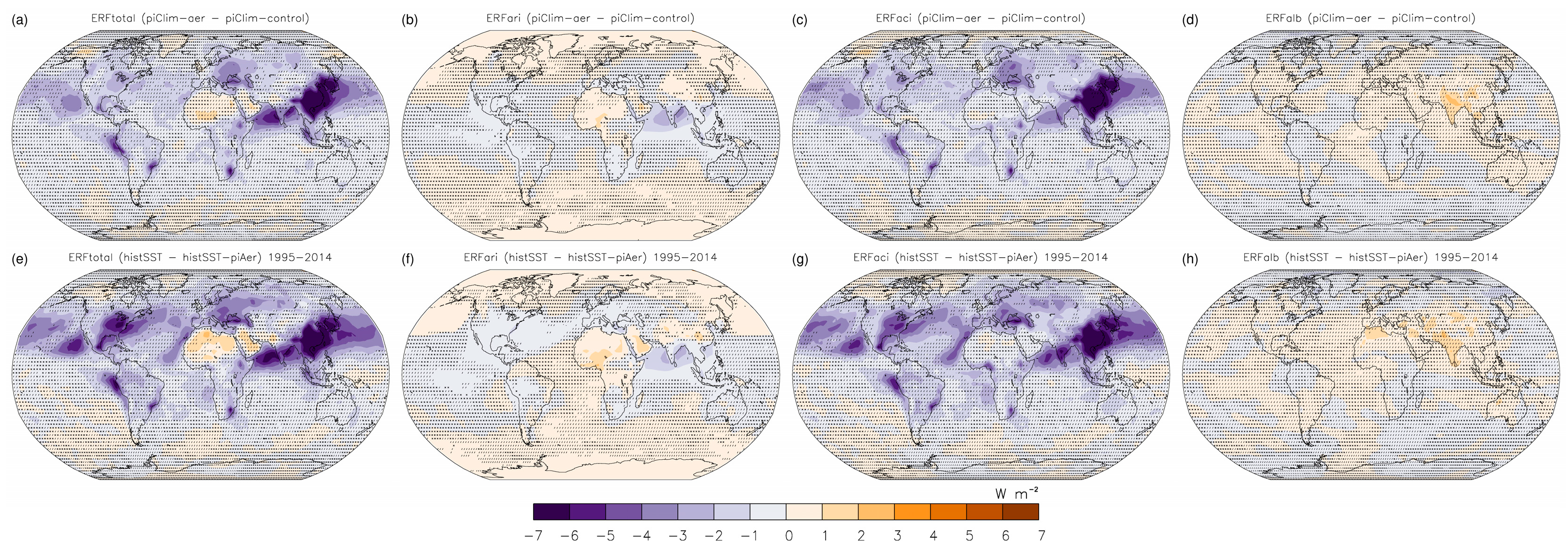
In Figure 1, the global mean ERF due to all aerosols based on piClim-aer and histSST (averaged over 1995–2014) experiments is presented. Both experiments exhibit a common spatial pattern for ERF at TOA. Aerosols induce a negative ERFtotal globally, mainly over the NH. The most negative values are detected over East and South Asia, whereas the most positive values can be found over reflective continental surfaces. ERFaci dominates ERFtotal on a global scale and exhibits a pattern almost identical to that of ERFtotal. ERFari is slightly negative globally, while the global mean ERFalb is slightly positive, peaking over the Himalayas and the Indian Peninsula.
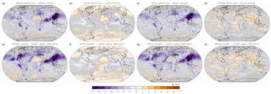
Figure 1.
(a,e) ERFtotal, (b,f) ERFari, (c,g) ERFaci, and (d,h) ERFalb pattern at TOA for piClim-aer (top row) and histSST (bottom row). Colored areas without markings indicate robust changes, while “/” and “X” symbols indicate non-robust changes and conflicting signals, respectively.
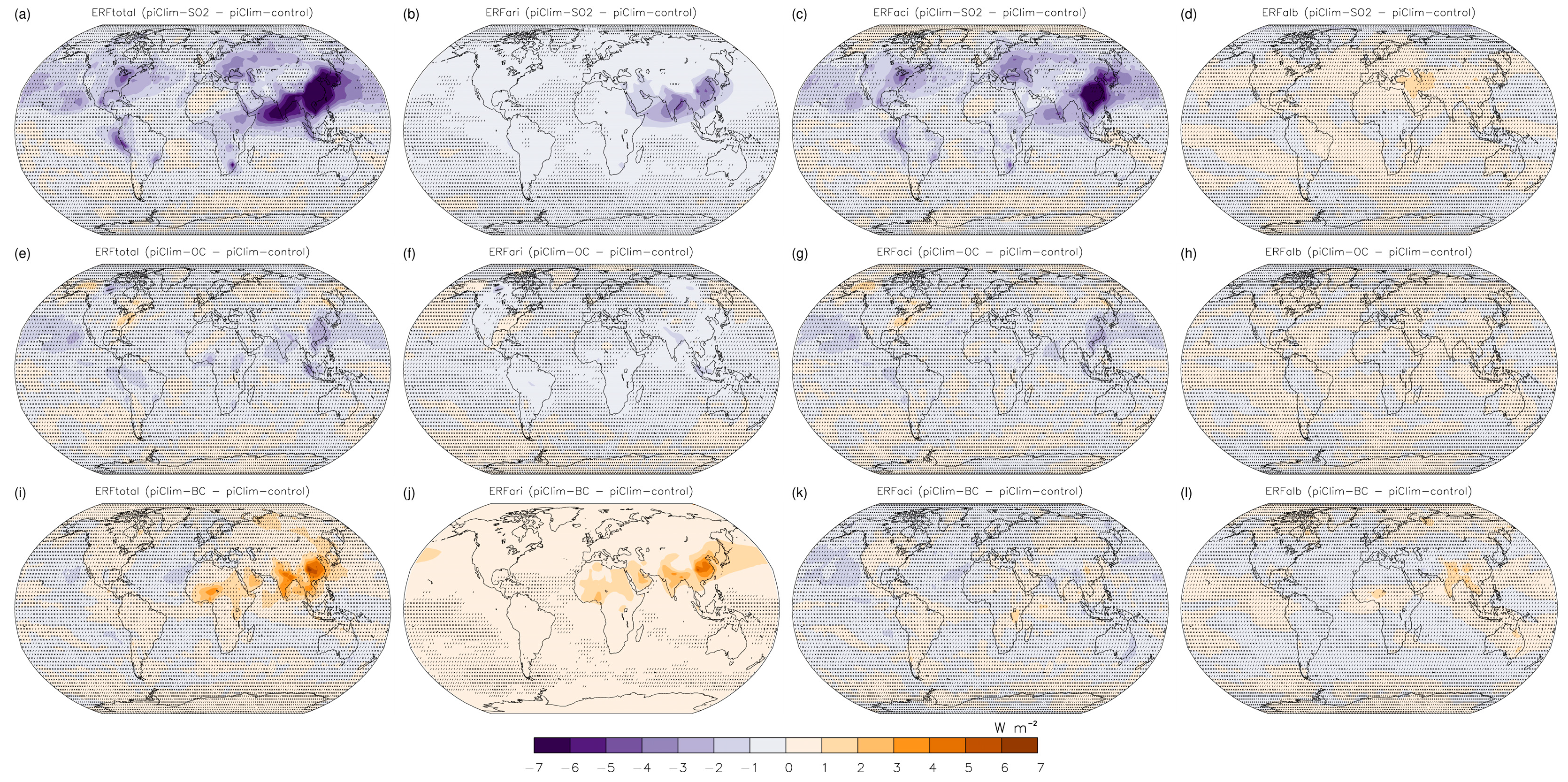
The decomposition of ERFtotal for piClim-BC, piClim-OC, and piClim-SO2 is presented in Figure 2.
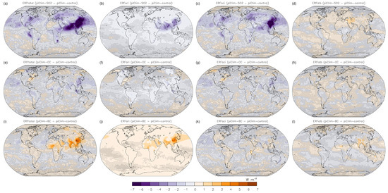
Figure 2.
(a,e,i) ERFtotal, (b,f,j) ERFari, (c,g,k) ERFaci, and (d,h,l) ERFalb pattern at TOA for piClim-SO2 (top row), piClim-OC (middle row), and piClim-BC (bottom row). Colored areas without markings indicate robust changes, while “/” and “X” symbols indicate non-robust changes and conflicting signals, respectively.
BC induces a positive global mean ERFtotal at TOA, peaking mainly over East and South Asia. The BC ERFtotal is driven by ERFari, which is positive all over the globe. Sulphates cause a negative global mean ERFtotal over the NH, especially over emission sources and downwind regions. As in the all-aerosol experiments, sulphate ERFaci drives the bulk of ERFtotal caused by sulphates. OC exerts a less negative global mean ERFtotal than sulphates, with negative peaks over Southeast Asia.
In Figure 3, the time evolution of ERFtotal and its components during the 1850–2014 period are shown for the entire globe and for five regions of interest from the IPCC AR6 ATLAS [12], namely East North America (ENA), Mediterranean (MED), West and Central Europe (WCE), South Asia (SAS), and East Asia (EAS), the boundaries of which are shown in the embedded map.
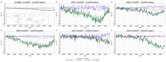
Figure 3.
Time evolution of the ERF components during 1850–2014. The results are shown for the histSST experiment on global scale (a), and over WCE (b), MED (c), ENA (d), SAS (e), and EAS (f).
Globally, aerosol ERF reaches its negative peak around 1980, with a trend towards more positive values by the end of the historical period. The dominant role of ERFaci is prominent, as it closely follows ERFtotal, while ERFari and ERFalb undergo much smaller changes. During the mid-1970s and early 1980s ERFtotal receives its most negative values over ENA, WCE, and MED. ERFtotal exhibits a strongly decreasing trend over EAS, while it shows a continuous increase in magnitude over SAS since the 1930s.
4. Conclusions
The ERF caused by anthropogenic aerosols was investigated using fixed-SST simulations from seven different ESMs participating in CMIP6 [9]. The total ERF was split into three main components (ERFari, ERFaci, ERFalb) using the method by Ghan [10]. All-aerosol ERFtotal is globally negative, mainly over the NH, with pronounced negative peaks over aerosol emission sources and downwind regions. Sulphates cause a negative ERFtotal globally and drive the spatial distribution of the all-aerosol radiative forcing at TOA. The OC ERFtotal is also negative, but much weaker in magnitude than the sulphate ERFtotal. On the other hand, BC exerts a globally positive ERFtotal driven by a strong ERFari all over the globe. Finally, changes in transient ERF were investigated on global scale and over five NH regions of interest during the 1850–2014 period. ERFtotal shows an increasing trend after 1980 over ENA, WCE, and MED, whereas ERFtotal shows a continuous decreasing trend over SAS and EAS after the 1950s.
Author Contributions
Conceptualization, P.Z., A.K.G. and D.A.; methodology, P.Z., A.K.G. and A.K.; software, A.K. and A.K.G.; formal analysis, A.K.; investigation, A.K., A.K.G. and P.Z.; data curation, A.K.; writing—original draft preparation, A.K.; writing—review and editing, A.K., A.K.G., D.A., R.J.A., V.N. and P.Z.; visualization, A.K., A.K.G. and P.Z.; supervision, P.Z.; project administration, P.Z. and A.K.G. All authors have read and agreed to the published version of the manuscript.
Funding
This research received no external funding.
Institutional Review Board Statement
Not applicable.
Informed Consent Statement
Not applicable.
Data Availability Statement
All data used in this study are freely available from the CMIP6 repository on the Earth System Grid Federation nodes (https://esgf-node.llnl.gov/search/cmip6/, accessed on 20 December 2022).
Acknowledgments
The authors acknowledge the World Climate Research Programme, which promoted and coordinated CMIP6 through its Working Group on Coupled Modelling. The authors thank the climate modelling groups (listed in Table 1) for producing and making available their model output, the Earth System Grid Federation (ESGF) for archiving the data and providing access, and the multiple funding agencies who support CMIP6 and ESGF.
Conflicts of Interest
The authors declare no conflict of interest.
References
- Boucher, O.; Randall, D.; Artaxo, P.; Bretherton, C.; Feingold, G.; Forster, P.; Kerminen, V.-M.; Kondo, Y.; Liao, H.; Lohmann, U.; et al. Clouds and Aerosols. In Climate Change 2013: The Physical Science Basis. Working Group I Contribution to the Fifth Assessment Report of the Intergovernmental Panel on Climate Change; Stocker, T.F., Qin, D., Plattner, G.-K., Tignor, M., Allen, S.K., Boschung, J., Nauels, A., Xia, Y., Bex, V., Midgley, P.M., Eds.; Cambridge University Press: Cambridge, UK; New York, NY, USA, 2013; pp. 571–658. [Google Scholar]
- Bellouin, N.; Quaas, J.; Gryspeerdt, E.; Kinne, S.; Stier, P.; Watson-Parris, D.; Boucher, O.; Carslaw, K.S.; Christensen, M.; Daniau, A.-L.; et al. Bounding Global Aerosol Radiative Forcing of Climate Change. Rev. Geophys. 2020, 58, e2019RG000660. [Google Scholar] [CrossRef]
- Szopa, S.; Naik, V.; Adhikary, B.; Artaxo Netto, P.E.; Berntsen, T.; Collins, W.D.; Fuzzi, S.; Gallardo, L.; Kiendler-Scharr, A.; Klimont, Z.; et al. Short-Lived Climate Forcers. In Climate Change 2021: The Physical Science Basis. Contribution of Working Group I to the Sixth Assessment Report of the Intergovernmental Panel on Climate Change; Masson-Delmotte, V., Zhai, P., Pirani, A., Connors, S.L., Péan, C., Berger, S., Caud, N., Chen, Y., Goldfarb, L., Gomis, M.I., et al., Eds.; Cambridge University Press: Cambridge, UK; New York, NY, USA, 2021; pp. 817–922. [Google Scholar]
- Lund, M.T.; Samset, B.H.; Skeie, R.B.; Watson-Parris, D.; Katich, J.M.; Schwarz, J.P.; Weinzierl, B. Short Black Carbon Lifetime Inferred from a Global Set of Aircraft Observations. npj Clim. Atmos. Sci. 2018, 1, 31. [Google Scholar] [CrossRef]
- Haywood, J.; Boucher, O. Estimates of the Direct and Indirect Radiative Forcing Due to Tropospheric Aerosols: A Review. Rev. Geophys. 2000, 38, 513–543. [Google Scholar] [CrossRef]
- Lohmann, U.; Feichter, J. Global Indirect Aerosol Effects: A Review. Atmos. Chem. Phys. 2005, 5, 715–737. [Google Scholar] [CrossRef]
- Ramaswamy, V.; Collins, W.; Haywood, J.; Lean, J.; Mahowald, N.; Myhre, G.; Naik, V.; Shine, K.P.; Soden, B.; Stenchikov, G.; et al. Radiative Forcing of Climate: The Historical Evolution of the Radiative Forcing Concept, the Forcing Agents and Their Quantification, and Applications. Meteorol. Monogr. 2019, 59, 14.1–14.101. [Google Scholar] [CrossRef]
- Forster, P.; Storelvmo, T.; Armour, K.; Collins, W.; Dufresne, J.-L.; Frame, D.; Lunt, D.J.; Mauritsen, T.; Palmer, M.D.; Watanabe, M.; et al. The Earth’s Energy Budget, Climate Feedbacks, and Climate Sensitivity. In Climate Change 2021: The Physical Science Basis. Contribution of Working Group I to the Sixth Assessment Report of the Intergovernmental Panel on Climate Change; Masson-Delmotte, V., Zhai, P., Pirani, A., Connors, S.L., Péan, C., Berger, S., Caud, N., Chen, Y., Goldfarb, L., Gomis, M.I., et al., Eds.; Cambridge University Press: Cambridge, UK; New York, NY, USA, 2021; pp. 923–1054. [Google Scholar]
- Eyring, V.; Bony, S.; Meehl, G.A.; Senior, C.A.; Stevens, B.; Stouffer, R.J.; Taylor, K.E. Overview of the Coupled Model Intercomparison Project Phase 6 (CMIP6) Experimental Design and Organization. Geosci. Model Dev. 2016, 9, 1937–1958. [Google Scholar] [CrossRef]
- Ghan, S.J. Technical Note: Estimating Aerosol Effects on Cloud Radiative Forcing. Atmos. Chem. Phys. 2013, 13, 9971–9974. [Google Scholar] [CrossRef]
- Collins, W.J.; Lamarque, J.-F.; Schulz, M.; Boucher, O.; Eyring, V.; Hegglin, M.I.; Maycock, A.; Myhre, G.; Prather, M.; Shindell, D.; et al. AerChemMIP: Quantifying the Effects of Chemistry and Aerosols in CMIP6. Geosci. Model Dev. 2017, 10, 585–607. [Google Scholar] [CrossRef]
- Gutiérrez, J.M.; Jones, R.G.; Narisma, G.T.; Muniz Alves, L.; Amjad, M.; Gorodetskaya, I.V.; Grose, M.; Klutse, N.A.B.; Krakovska, S.; Li, J.; et al. Atlas. In Climate Change 2021: The Physical Science Basis. Contribution of Working Group I to the Sixth Assessment Report of the Intergovernmental Panel on Climate Change; Masson-Delmotte, V., Zhai, P., Pirani, A., Connors, S.L., Péan, C., Berger, S., Caud, N., Chen, Y., Goldfarb, L., Gomis, M.I., et al., Eds.; Cambridge University Press: Cambridge, UK; New York, NY, USA, 2021; pp. 1927–2058. [Google Scholar]

Disclaimer/Publisher’s Note: The statements, opinions and data contained in all publications are solely those of the individual author(s) and contributor(s) and not of MDPI and/or the editor(s). MDPI and/or the editor(s) disclaim responsibility for any injury to people or property resulting from any ideas, methods, instructions or products referred to in the content. |
© 2023 by the authors. Licensee MDPI, Basel, Switzerland. This article is an open access article distributed under the terms and conditions of the Creative Commons Attribution (CC BY) license (https://creativecommons.org/licenses/by/4.0/).