Abstract
High horizontal resolution regional climate model simulations serve as forcing data for crop and dynamic vegetation models, for generating possible scenarios of the future effects of climate change on crop yields and pollinators. Here, we performed convection-permitting hindcast simulations with the regional climate model COSMO5.0-CLM15 (CCLM) from 1979 to 2015, and the first year was considered as a spin-up period. The model was driven with hourly ERA5 data, which were the latest climate reanalysis product by ECMWF, and directly downscaled to a 3 km horizontal resolution over Central Europe. The land-use classes were described by ECOCLIMAP, and the soil type and depth were described by HWSD. The evaluation was carried out in terms of temperature, precipitation, and climate indices, comparing CCLM output with the gridded observational dataset HYRAS from the German Weather Service. While CCLM inherits a warm and dry summer bias found in its parent model, it reproduces the main features of the recent past climate of Central Europe, including the seasonal mean climate patterns and probability density distributions. Furthermore, the model reproduced climate indices for temperature like growing season length, growing season start date, number of summer days. The results highlighted the possibility of directly downscaling ERA5 data with regional climate models, avoiding the multiple nesting approach and high computational costs. This study adds confidence to convection-permitting climate projections of future changes in agricultural climate indices.
1. Introduction
Climate change is occurring at a fast pace. Many sectors are affected by present and future global warming, which is projected by climate models. Climate change information is needed at regional and local scales for adaption and mitigation strategies. Furthermore, future scenarios concerning the effects of climate change on crop yields and pollinators are still in its infant shoes. One reason among others is that the climate forcing data of a regional climate model to drive dynamic vegetation models are too coarse to generate local scale yield estimates, and a large precipitation bias compared to observational data of about 40% is inherent in the coarse climate model data [1]. Statistical bias correction of the forcing data for impact models introduces another uncertainty into the local weather statistics.
The horizontal resolution of regional climate models decreased in the recent past decades in a coordinated ensemble of climate simulations, projects from 50 km (PRUDENCE project [2]) to 25 km (ENSEMBLES project) and 12 km (PRINCIPLES and EURO-CORDEX project [3]). These projects assessed the uncertainty of RCM projections and impact assessment studies, by evaluating the systematic model behavior and biases [4] found only small differences in seasonal mean quantities between 50 km and 12 km horizontal resolution simulations. At the same time, convection-permitting simulations emerged at a kilometer-scale grid [5]. These studies were conducted for the recent past, as well as for projected future conditions and over different geographical regions at horizontal resolutions below 4 km, in which deep convection parameterization was switched off. Improvements were shown for land-atmosphere couplings, temperature representation, the timing and diurnal cycle of precipitation, and the spatial structure of temperature and precipitation [6,7,8,9].
Convection-permitting regional climate models at a few kilometers scale offer a tool to force dynamic vegetation models at local and regional scales on climate time scales without bias correction, assuming that the bias is in the uncertainty range of observations. Such high horizontal resolution simulations realistically capture convection and snowfall in Europe [1,10,11] and over the Rocky Mountains in the U.S. [12,13]. Investigations of climate and climate change impacts on yields and biodiversity would benefit from such high-resolution simulations at the climate time scale.
Inherent are the computational costs of such high horizontal resolution simulations. Multiple nesting steps are performed to reach the kilometer scale. A way around would be direct downscaling experiments. The first results of direct downscaling simulations forced by ERA-Interim reanalysis generated realistically different convection events over an extended domain, covering the Alps in Europe [1]. This is a promising way forward for reducing computational costs.
Multisectoral analysis of climate and land-use change impacts on pollinators, plant diversity, and crops yields (MAPPY) project, for the first time, combines diverse research sectors in a coordinated manner, using convection-permitting simulations for impact assessments on crop yields and pollinators. Central Europe and Spain were defined as target areas for these experimental efforts.
In this manuscript, we present the first multi-decade climate evaluation simulations at a convection-permitting resolution, using ERA5 reanalysis as forcing. The main goal was to evaluate this multi-decade-long simulation against available high-resolution observations. Here, we show the benefit of convection-permitting simulations from the direction downscaling experiments for agricultural-related climate indices over Central Europe. ERA5 reanalysis data were directly downscaled with the regional climate model COSMO-CLM [14], for the period of 1980 to 2015.
Section 2 of this manuscript represents the regional climate model, data, and methods used in this study. In Section 3, results on the evaluation of precipitation and temperature and their agricultural-related climate indices are provided and discussed. Summary and conclusions are provided in Section 4.
2. Methods
2.1. Model
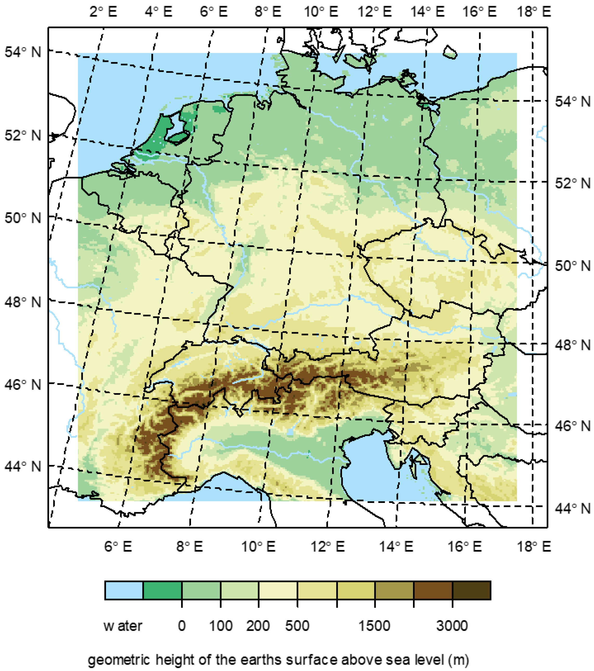
Simulations were conducted as a direct downscaling experiment at a convection-permitting horizontal resolution (about 3 km) over Central Europe, within the frame of MAPPY. The region of the simulation domain is shown in Figure 1. The limited-area model used in this study was the COSMO model [15] in climate mode [14], designed for applications for the meso-β to the meso-γ scales. The version used was COSMO-CLM v5.15. The selection of different dynamical and physical parameterization schemes allowed the application of the model for a wide range of spatial and temporal scales. The model integrated the fully compressible, non-hydrostatic thermo-dynamical equations in a moist atmosphere. The equations were solved numerically on an Arakawa-C staggered grid [16] in rotated coordinates, with a Runge-Kutta time-stepping scheme [17]. The model used a vertical terrain-following height coordinate [18]. A one-moment microphysics scheme including five categories of hydrometeors (cloud, rain, snow, ice, and graupel) was used for the parameterization of precipitation. Soil processes were presented by the multi-layer soil model TERRA-ML [19]. The simulations used a modified Tiedtke parameterization of shallow convection. Deep convection was switched off, allowing the resolution of convective processes. The radiative transfer scheme was based on [20], and a turbulent kinetic energy-based surface transfer and planetary boundary layer parameterization [21] was applied. The land-use classes were described by ECOCLIMAP, and the soil type and depth by HWSD.
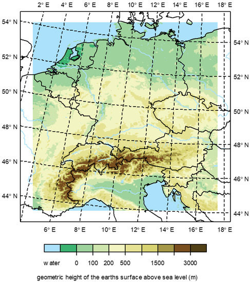
Figure 1.
Orography of the model domain covering Central Europe, without the sponge zone.
Simulation results were investigated for performance under present-day climate conditions. Thus, hourly ERA5 reanalysis [22] were downscaled for multiple decades from 1980 to 2015. ERA5 is the fifth-generation model reanalysis of the global climate from the European Centre for Medium-range Weather Forecasts (ECMWF). The spin-up year 1979 was excluded from the analysis. A region of 23 grid points at each side was removed to exclude any lateral boundary artifacts.
2.2. Statistical Analysis
High-resolution observational precipitation and temperature datasets were used for the evaluation analysis. The daily gridded datasets at five-kilometer horizontal resolution were from HYRAS [23], which was available over entire Germany and the adjacent regions covering the period 1951–2015. It was generated using station data. Note that gridded observational data included a bias in real observations. Shortcomings, for example, could be associated with underestimation of precipitation or using interpolation methods.
Simulated temperature and precipitation were evaluated for absolute and relative biases, respectively, relative to the observations. The region selected depended on the coverage of the observational data of HYRAS. The absolute bias was the difference of model minus observations. The relative bias was the difference of model minus observations divided by observations. The simulation results were remapped to the observational grid using bi-linear remapping before the analysis. This ensured a grid-cell-by-grid-cell comparison between model and observations.
The analysis was done for the climate indices listed in Table 1. These climate indices for temperature and precipitation were related to droughts, floods, heat/cold waves, and agriculture-specific events. We evaluated the CCLM simulation based on these indices. Often the RMSE (root-mean-square error) between the simulations and the observations was calculated to reflect the quality of simulations. As the selected indices had different units and ranges, here we calculated the standardized RMSE, which was adopted from [24].
where g indicates grid point; I indicates the given index, obs is the observational data, and sim is the simulations data. The climate index was rated as well-performing when the standardized RMSE value was below 0.5, and as biased otherwise, as suggested by [24].

Table 1.
Description and definition of the climate indices used in this study. (PR: daily precipitation; TX: daily maximum temperature; TN: daily minimum temperature; and TG: daily mean temperature).
3. Results and Discussion
Here, we showed the evaluation results between the simulated climate variables (temperature and precipitation) and the observed ones, concerning the annual cycle, spatial distribution, PDF (probability density function), and the above-mentioned climate indices.
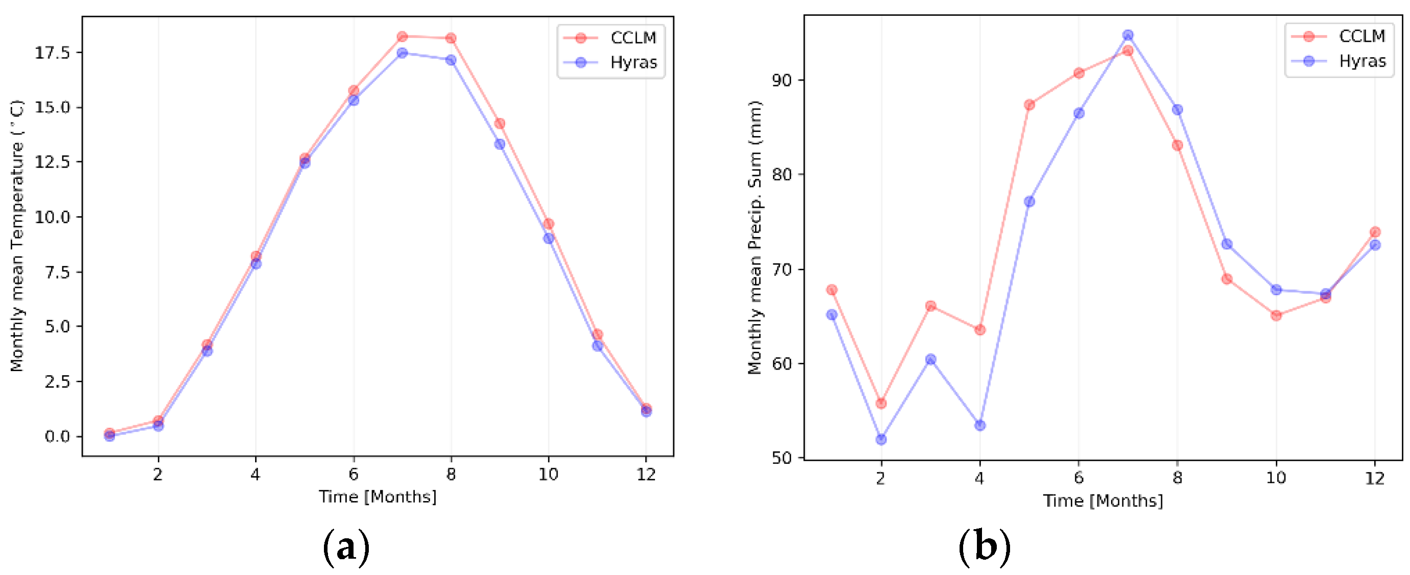
The observed annual cycle was well reproduced in the model, with a small bias range (Figure 2). The temperature biases ranged between 0–1.0 °C, depending on the season and the precipitation biases range between −5% and 20%. In detail, the simulated summer tended to be 0.5–1.0 °C warmer than the observed one, and the simulated winter was almost as cold as the observed one (biases below 0.3 °C). For precipitation, the modeled spring season tended to be wetter (10–20%) and the autumn tended to be slightly drier (biases within −10%).
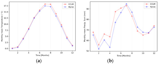
Figure 2.
Annual cycle of (a) temperature (°C) and (b) precipitation (mm/month) for model simulations and observation data.
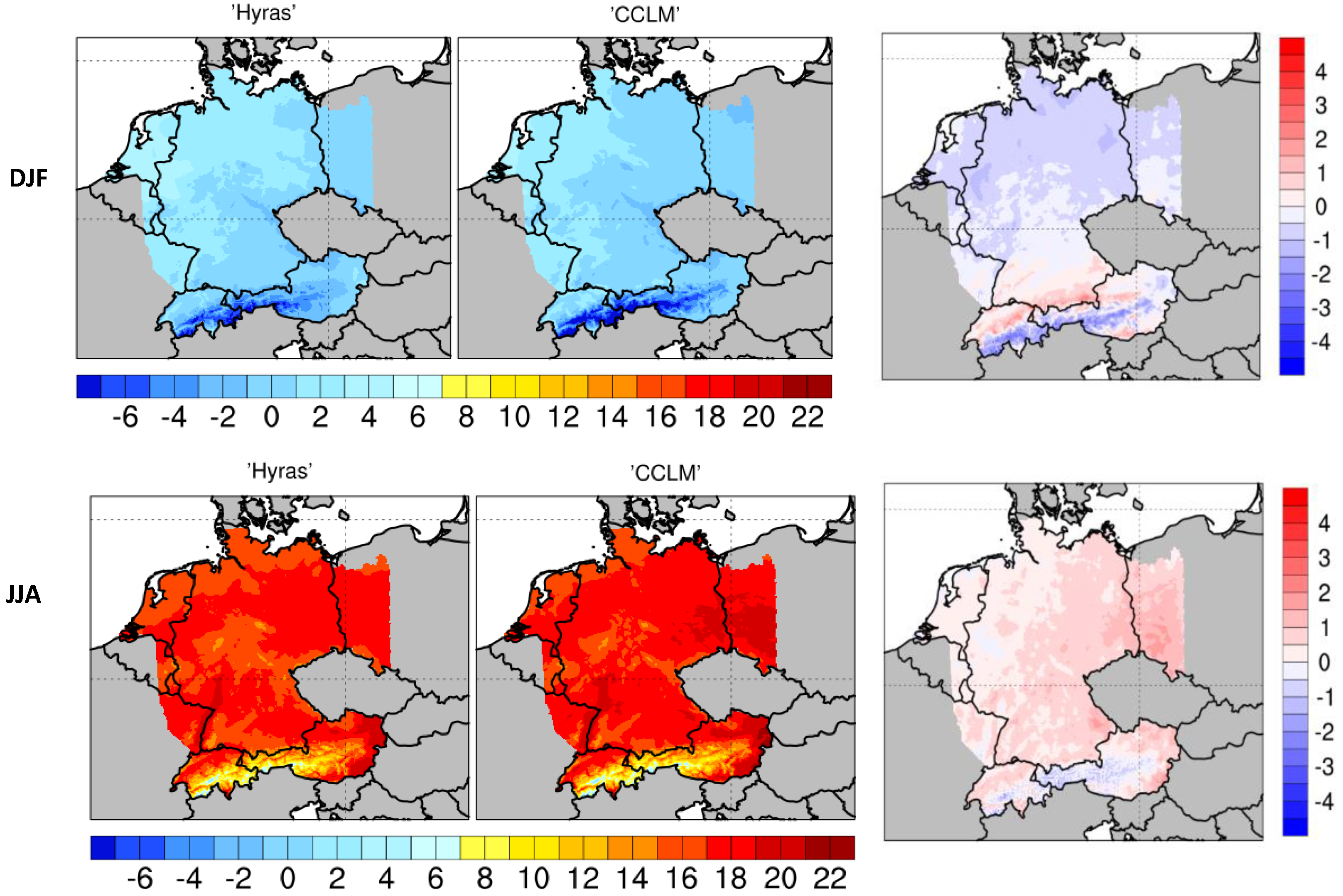
The spatial distribution of daily precipitation and temperature showed good agreement with model simulations (Figure 3 and Figure 4). The results are presented for the winter and summer seasons. Most of the northern region tended to be colder in winter (biases within 1.0 °C) and slightly warmer in summer (biases within 0.5 °C). The northern part of the Alps was constantly warmer and the southern part of the Alps was colder in the model (biases ranged between −2 °C and 2 °C). For precipitation, the most western part of the domain tended to be drier and the eastern part was wetter in the model, and the Alps region showed the highest wet biases. The bias was higher in the winter season than in summer. The winter season was dominated by mid-latitude storms, whereas isolated, convective events occurred in the summer season. High precipitation in the model simulations occurred in regions with high orography in both winter and summer. Some of these biases might be inherited by the driving model.

Figure 3.
The spatial pattern of mean seasonal temperature for the observation and the simulation (left panel) and mean seasonal temperature bias (Tcclm-Thyras, °C) for the period 1980–2015. Upper rows—winter (DJF), and lower rows—summer (JJA).
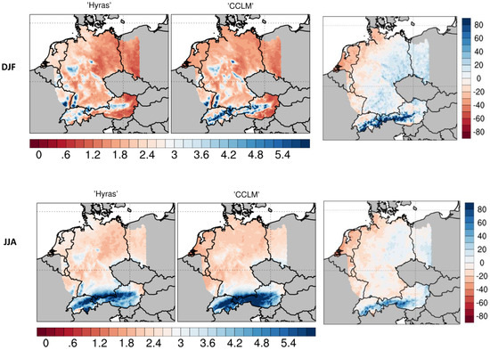
Figure 4.
As Figure 3 but for spatial pattern of daily precipitation and the mean relative seasonal precipitation bias ((Pcclm-Phyras)/Phyras, %).
Simulated precipitation amounts were higher over the Alps, especially in winter, as compared to observations. Precipitation all year round and snow in winter was difficult to measure in the Alps. Furthermore, wind introduced a systematic rain gauge under-catch. Most stations in mountainous regions were located in valleys, which increased the uncertainty estimates of the mountain top and particularly the mountain slopes. This might be the reason why the observations seemed to be lower over the Alps, as compared to the 3 km simulation. Recent studies showed that the 3 km model might estimate snowfall better than observations due to its ability to capture the main vertical motion associated with snow formation at these scales [25] and improvements in the microphysical parameterizations [26].
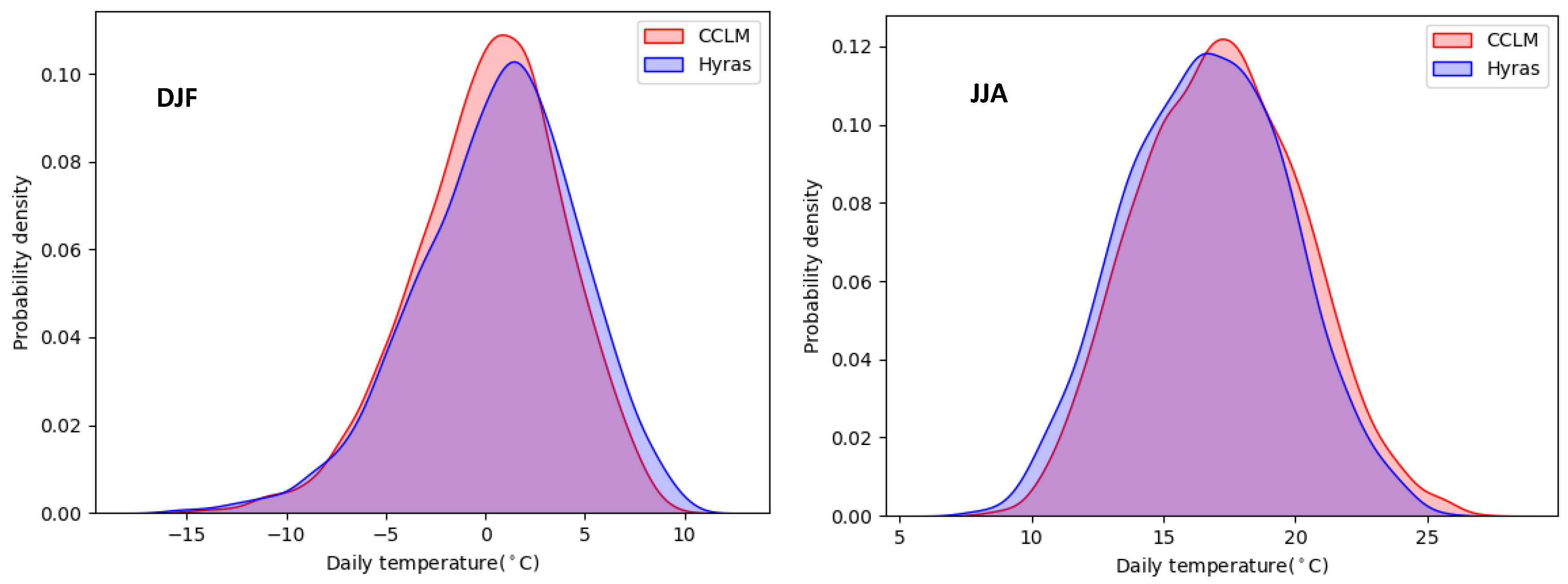
Figure 5 and Figure 6 show the PDF (probability density function) of averaged daily temperature and precipitation over the domain, in the winter and summer seasons. The domain experienced slightly fewer warm events in the winter season and less cold- and more warm events in the summer season in the model. The simulation well reproduced the PDF of the observed precipitation events in the winter season. In the summer season, the model generated more extreme precipitation than the observations.

Figure 5.
Probability density function of simulated (red) and observed (blue) daily mean temperature over the domain. Left—winter (DJF), right—summer (JJA).
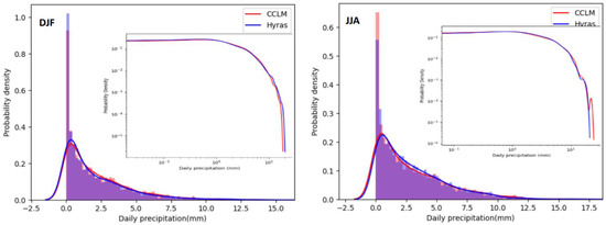
Figure 6.
Probability density function of simulated (red) and observed (blue) daily precipitation over the domain. Left—winter (DJF), right—summer (JJA).
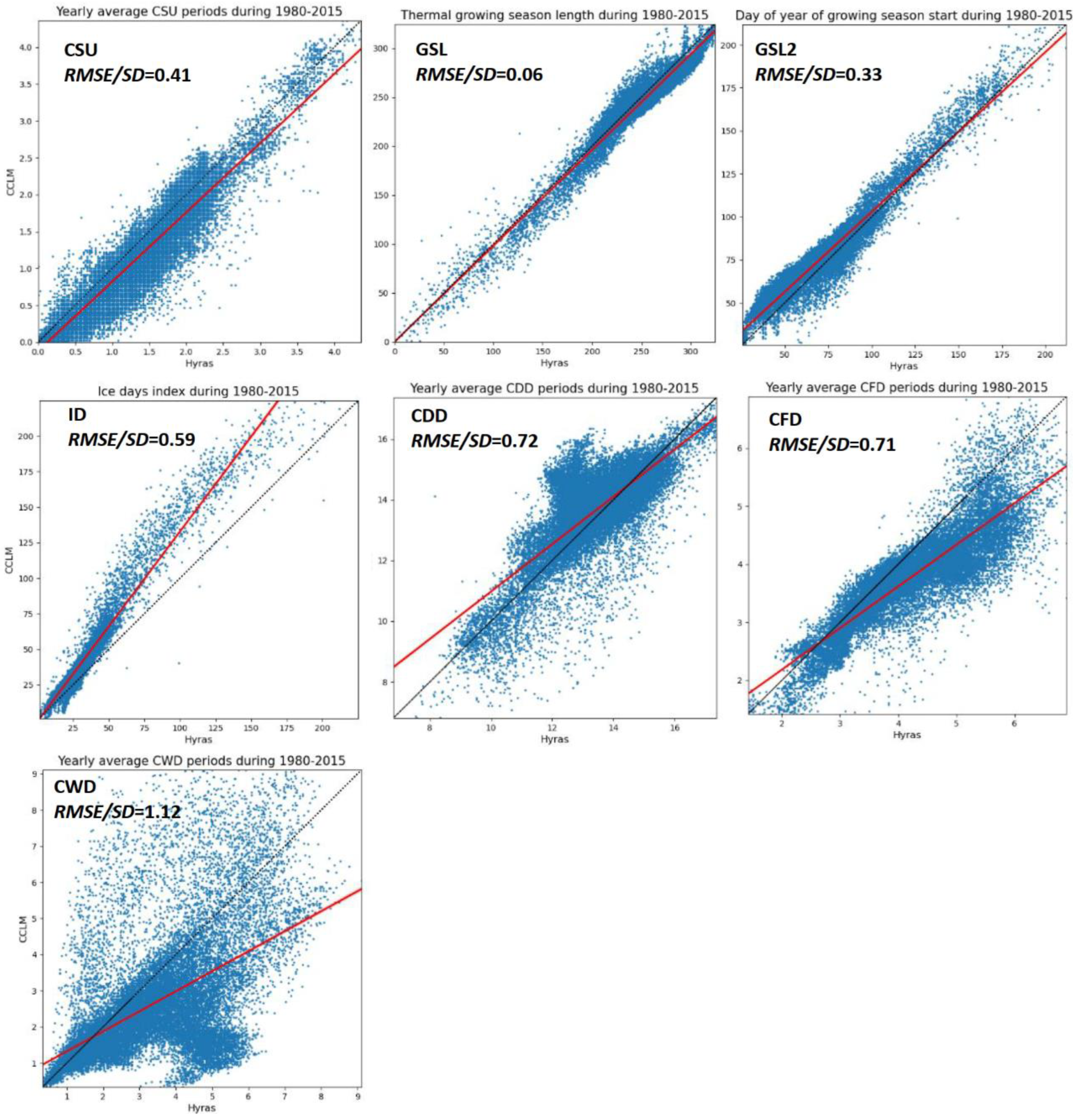
Both the starting day of the growing season and the growing season length revealed a good performance with standardized RMSEs below 0.5, see Figure 7. Heatwave events (indicated by CSU) were well captured in the model with standardized RMSEs also below 0.5. Meanwhile, the model tended to generate fewer cold waves and droughts at most grid points (the simulated CDD and CFD values were smaller than the observed ones). The simulated ice days occurred more frequently than in the observations. The model somehow failed to capture the floods, as the simulated CWD was different from the observed ones at many grid points.

Figure 7.
Evaluation of the climate indices, shown as scatter plots of observed (x-axis) and simulated (y-axis) values during 1980–2015. The indicated performance metric is defined as the standardized RMSE divided by the standard deviation of observed values across grid points (RMSE/SD < 0.5: well simulated; RMSE/SD > 0.5: relatively worse performance). Redline—the linear trend; the black dashed line—the perfect correlation between observed and simulated data.
Generally, the analysis showed that in most regions and for most indices the uncertainty ranges were small for convection-permitting simulations. The spatial representation of precipitation and temperature was very similar to observations.
4. Summary and Conclusions
Simulated precipitation and temperature were evaluated against observations in this study for their biases and agricultural-related climate indices of a new high-resolution climate simulation, with a direct-downscaling approach at a 3 km horizontal resolution. The simulation was driven by ERA5 reanalysis integrated over a 36-year long period. The model performance was analyzed by the absolute and relative biases and indices, which are important for agriculture. Generally, the spatial patterns and variability were well represented by the kilometer-scale simulation on daily time scales. The uncertainty ranges were reduced by half with this high-resolution simulation, as compared to the EURO-CORDEX simulations with a coarser horizontal resolution, see [4]. The benefit of convection-permitting simulations was that the model got rid of the uncertainty due to the deep convection scheme since the deep convection parameterization was switched off. A more realistic orography and land-use added further value to kilometer-scale simulations for providing local-scale climate information.
The direct downscaling simulations performed realistically and could be recommended without the intermediate nest. Downscaling directly from reanalysis without an intermediate nest has a high downscaling ratio, and could introduce significant lateral boundary artifacts. However, since the lateral boundaries were far away, and the simulation domain was big enough, it was not an issue.
Further simulations and analysis are to be performed over Spain and the future period, until 2070.
Institutional Review Board Statement
Not applicable.
Informed Consent Statement
Not applicable.
Acknowledgments
The project MAPPY is part of AXIS, an ERA-NET initiated by JPI Climate, and funded by national agencies (DLR/BMBF, DE, Grant No. 01LS1907A-C) with co-funding by the Horizon 2020 - the Framework Programme for Research and Innovation (2014-2020) of the European Union. Computational resources were made available by the German Climate Computing Center (DKRZ) through support from the German Federal Ministry of Education and Research (BMBF). This research was done in collaboration with the CLM-community.
References
- Ban, N.; Brisson, E.; Caillaud, C.; Coppola, E.; Pichelli, E.; Sobolowski, S.; Adinolfi, M.; Alias, A.; Anders, I.; Bastin, S.; et al. The first multi-model ensemble of regional climate simulations at the kilometer-scale resolution, Part I: Evaluation of precipitation. Clim. Dyn. 2021, 57, 275–303. [Google Scholar] [CrossRef]
- Christensen, J.; Carter, T.; Mea, R. Evaluating the performance and utility of regional climate models: The PRUDENCE project. Clim. Chang. 2007, 81, 1–6. [Google Scholar] [CrossRef]
- Giorgi, F. Thirty years of regional climate modeling: Where are we and where are we going next? J. Geophys. Res. Atmos. 2019, 124, 5696–5723. [Google Scholar] [CrossRef]
- Kotlarski, S.; Keuler, K.; Christensen, O.B.; Colette, A.; Deque, M.; Gobiet, A.; Goergen, K.; Jacob, D.; Luüthi, D.; van Meijgaard, E.; et al. Regional climate modeling on European scales: A joint standard evaluation of the EURO-CORDEX RCM ensemble. Geosci. Model. Dev. Discuss. 2014, 7, 217–293. [Google Scholar] [CrossRef]
- Prein, A.F.; Langhans, W.; Fosser, G.; Ferrone, A.; Ban, N.; Goergen, K.; Keller, M.; Tölle, M.; Gutjahr, O.; Feser, F.; et al. A review on regional convection-permitting climate modeling: Demonstrations, prospects, and challenges. Rev. Geophys. 2015, 53, 323–361. [Google Scholar] [CrossRef] [PubMed]
- Kendon, E.J.; Roberts, N.M.; Fowler, H.J.; Roberts, M.J.; Chan, S.C.; Senior, C.A. Heavier summer downpours with climate change revealed by weather forecast resolution model. Nat. Clim. Chang. 2014, 4, 570–576. [Google Scholar] [CrossRef]
- Ban, N.; Schmidli, J.; Schaär, C. Evaluation of the convection-resolving regional climate modeling approach in decade-long simulations. J. Geophys. Res. Atmos. 2014, 119, 7889–7907. [Google Scholar] [CrossRef]
- Tölle, M.H.; Gutjahr, O.; Thiele, J.; Busch, G. Increasing bioenergy production on arable land: Does the regional and local climate respond? J. Geophys. Res. Atmos. 2014, 119, 2711–2724. [Google Scholar] [CrossRef]
- Tölle, M.H.; Schefczyk, L.; Gutjahr, O. Scale dependency of regional climate modeling of current and future climate extremes in Germany. Theor. Appl. Climatol. 2018, 134, 829–848. [Google Scholar] [CrossRef]
- Leutwyler, D.; Luüthi, D.; Ban, N.; Fuhrer, O.; Schär, C. Evaluation of the convection-resolving climate modeling approach on continental scales. J. Geophys. Res.-Atmos. 2017. [Google Scholar] [CrossRef]
- Coppola, E.; Sobolowski, S.; Pichelli, E.; Raffaele, F.; Ahrens, B.; Anders, I.; Ban, N.; Bastin, S.; Belda, M.; Belusic, D.; et al. A first-of-its-kind multi-model convection permitting ensemble for investigating convective phenomena over europe and the mediterranean. Clim. Dyn. 2020, 1–32. [Google Scholar] [CrossRef]
- Rasmussen, R.; Liu, C.; Ikeda, K.; Gochis, D.; Yates, D.; Chen, F.; Tewari, M.; Barlage, M.; Dudhia, J.; Yu, W.; et al. High-resolution coupled climate runoff simulations of seasonal snowfall over colorado: A process study of current and warmer climate. J. Clim. 2011, 24, 3015–3048. [Google Scholar] [CrossRef]
- Liu, C.; Ikeda, K.; Rasmussen, R.; Barlage, M.; Newman, A.J.; Prein, A.F.; Chen, F.; Chen, L.; Clark, M.; Dai, A.; et al. Continental-scale convection-permitting modeling of the current and future climate of North America. Clim. Dyn. 2017, 49, 71–95. [Google Scholar] [CrossRef]
- Rockel, B.; Will, A.; Hense, A. The regional climate model COSMO-CLM (CCLM). Meteorologische Zeitschrift 2008, 17, 347–348. [Google Scholar] [CrossRef]
- Baldauf, M.; Seifert, A.; Förstner, J.; Majewski, D.; Raschendorfer, M.; Reinhardt, T. Operational convection-scale numerical weather prediction with the COSMO model: Description and sensitivities. Mon. Weather Rev. 2011, 139, 3887–3905. [Google Scholar] [CrossRef]
- Arakawa, A.; Lamb, V. Computational design of the basic dynamical processes in the UCLA general circulation model. In Methods in Computational Physics: General Circulation Models of the Atmosphere; Chang, J., Ed.; Academic Press: New York, NY, USA, 1977; Volume 17, pp. 173–265. [Google Scholar] [CrossRef]
- Wicker, L.J.; Skamarock, W.C. Time-Splitting Methods for Elastic Models Using Forward Time Schemes. Mon. Weather Rev. 2002, 130(8), 2088–2097. [Google Scholar] [CrossRef]
- Doms, G.; Baldauf, M. A Description of the Non-Hydrostatic Regional COSMO Model, Part I: Dynamics and Numerics; Offenbach: Germany, 2015. [Google Scholar]
- Schrodin, E.; Heise, E. A New Multi-Layer Soil Model; COSMO Newsletter No. 2:149–151; German Weather Service: Offenbach: : Germany, 2002. [Google Scholar]
- Ritter, B.; Geleyn, J.F. A comprehensive radiation scheme for numerical weather prediction models with potential applications in climate simulations. Mon. Weather Rev. 1992, 120, 303–325. [Google Scholar] [CrossRef]
- Raschendorfer, M. The New Turbulence Parametrization of LM; COSMO Newsletter No. 1:90-98; German Weather Service: Offenbach: Germany, 2001. [Google Scholar]
- Hersbach, H.; de Rosnay, P.; Bell, B.; Schepers, D.; Simmons, A.; Soci, C.; Abdalla, S.; Alonso-Balmaseda, M.; Balsamo, G.; Bechtold, P.; et al. Operational Global Reanalysis: Progress, Future Directions and Synergies with NWP; ERA Report Series 27; ECMWF: Reading, UK, 2018. [Google Scholar]
- Razafimaharo, C.; Krähenmann, S.; Höpp, S.; Rauthe, M.; Deutschländer, T. New high-resolution gridded dataset of daily mean, minimum, and maximum temperature and relative humidity for Central Europe (HYRAS). Theor. Appl. Climatol. 2020, 142, 1531–1553. [Google Scholar] [CrossRef]
- Tschurr, F.; Feigenwinter, I.; Fischer, A.M.; Kotlarski, S. Climate Scenarios and Agricultural Indices: A Case Study for Switzerland. Atmosphere 2020, 11, 535. [Google Scholar] [CrossRef]
- Lundquist, J.; Hughes, M.; Gutmann, E.; Kapnick, S. Our Skill in Modeling Mountain Rain and Snow is Bypassing the Skill of Our Observational Networks. Bull. Am. Meteorol. Soc. 2020, 100, 2473–2490. [Google Scholar] [CrossRef]
- Liu, X.; Xie, S.; Boyle, J.; Klein, S.A.; Shi, X.; Wang, Z.; Lin, W.; Ghan, S.J.; Earle, M.; Liu, P.S.K.; et al. Testing cloud microphysics parameterizations in NCAR CAM5 with ISD AC and M-PACE observations. J. Geophys. Res. 2011, 116. [Google Scholar] [CrossRef]
Publisher’s Note: MDPI stays neutral with regard to jurisdictional claims in published maps and institutional affiliations. |
© 2020 by the authors. Licensee MDPI, Basel, Switzerland. This article is an open access article distributed under the terms and conditions of the Creative Commons Attribution (CC BY) license (https://creativecommons.org/licenses/by/4.0/).

