Integrated Parametric Graph Closure and Branch-and-Cut Algorithm for Open Pit Mine Scheduling under Uncertainty

Abstract

Open pit mine production scheduling is a computationally expensive large-scale mixed-integer linear programming problem. This research develops a computationally efficient algorithm to solve open pit production scheduling problems under uncertain geological parameters. The proposed solution approach for production scheduling is a two-stage process. The stochastic production scheduling problem is iteratively solved in the first stage after relaxing resource constraints using a parametric graph closure algorithm. Finally, the branch-and-cut algorithm is applied to respect the resource constraints, which might be violated during the first stage of the algorithm. Six small-scale production scheduling problems from iron and copper mines were used to validate the proposed stochastic production scheduling model. The results demonstrated that the proposed method could significantly improve the computational time with a reasonable optimality gap (the maximum gap is 4%). In addition, the proposed stochastic method is tested using industrial-scale copper data and compared with its deterministic model. The results show that the net present value for the stochastic model improved by 6% compared to the deterministic model.

1. Introduction

Open pit mine production scheduling is a multicycle priority constraint knapsack problem, usually suitable for mixed-integer linear programming (MILP) frameworks [1,2]. The production schedule begins with the geological block model, which is represented as a three-dimensional array of blocks. Each block represents the volume of material that can be mined. The size of the blocks in the block model is determined considering the exploration drilling patterns, geological conditions, and the size of the mining equipment to be used. The information obtained from the exploration drilling is used to interpolate weight and metal content for each block [3].

For production scheduling, the mining blocks are represented by their weights, economic values (net profit from the block), ore contents (weight of the block with positive economic value), and metal contents (amount of metal released after processing ore block). During production scheduling, several decisions are made to maximize the profit, e.g., whether a given block will be mined or not, when it will be mined, etc. [4]. Once a block is specified for mining, a different destination or processing method may be determined for the block. The process of determining the time and the order of extraction by period is called mine production scheduling [5].

During production scheduling, mining blocks are assigned to different periods to maximize total discounted profits during the mining life, subject to operational constraints. These constraints are slope angle, mining capacity, processing capacity, and many more. Production scheduling in open pit mines is a complex task, especially for a large number of mining blocks and significant life of mine [6]. Typically, open pit mine production scheduling is addressed by mixed integer programming [6,7]. However, finding the best production plan is always a complex task due to a large number of integer variables and constraints. Moreover, the mining reserve estimation process is associated with both internal and external uncertainties, making the mining project a risky investment decision. The complexity of the problem is further increased with these uncertainties associated with the different parameters of the mining block.

Traditionally, the mine production scheduling problem is solved for deterministic models without considering any uncertainties associated with the deposits, leading to the inaccurate deposit assessment [8,9,10,11,12]. However, uncertainties and risks are well understood within the mining community. Therefore, stochastic models attract more attention as they are more realistic and relevant to dealing with uncertainty and risk. One standard approach to solve the stochastic problems is to evaluate the revenue at different scenarios and minimize deviations from the production targets [7,13,14,15]. Dimitrakopoulos et al. [16] solved the mine production scheduling problem under grade uncertainty by capturing maximum potential and minimizing downside risk. Abdel Sabour et al. [13] solved the stochastic mine production scheduling problem using a ranking system for selecting technically feasible mine designs under grade uncertainty and operating flexibility. Boland et al. [17] reduced the geological risk using a multistage stochastic programming approach. Dimitrakopoulos and Ramazan [18] optimized a mine production scheduling problem using stochastic integer programming to consider grade uncertainty. Dimitrakopoulos [19] developed robust stochastic schedules to maximize the NPV and metal production and minimize not meeting targets and related losses by integrating stochastic modeling for grade uncertainty. Groeneveld and Topal [20] solved the stochastic mine production scheduling problem by combining mixed-integer programming and Monte Carlo simulation to increase the flexibility of the mine design. Lamghari and Dimitrakopoulos [11] solved a production scheduling problem under metal uncertainty using Tabu search. Leite and Dimitrakopoulos [21] used a stochastic scheduling approach based on simulated annealing to generate a production schedule under grade uncertainty. Ramazan and Dimitrakopoulos [7] proposed a two-stage stochastic integer programming (SIP) model to maximize the net present value (NPV) of the production plan while minimizing the risk of nonconforming production targets. Khan and Niemann-Delius [22] used particle swarm optimization, and Shishvan and Sattarvand [23] used ant colony optimization for long-term production planning. Goodfellow and Dimitrakopoulos [24] proposed the global optimization of open pit mine extraction sequence under grade uncertainty by using a combination of particle swarm optimization, sequential annealing, and differential evolution.

Recently, different hybrid algorithms have been introduced to solve mine production scheduling problems. Montiel and Dimitrakopoulos [25] demonstrated with a copper mine dataset that the hybrid method could increase the expected net present value by 30% compared to a solution generated with standard industry practice. Two different metaheuristic techniques based on particle swarm optimization (PSO) and the bat algorithm are proposed to solve the stochastic open pit mine scheduling problem [26]. A new hyper-heuristic algorithm that combines elements from reinforcement learning and tabu search is introduced by Lamghari and Dimitrakopoulos [27], which shows improvement in solution quality and computational time. Paithankar and Chatterjee [28] present a hybrid method using maximum flow and genetic algorithm to determine the optimal extraction sequence. Their results with benchmark datasets show the hybrid method can improve production scheduling performance. Chatterjee and Dimitrakopoulos [29] proposed a new method for open pit mine production scheduling under geological uncertainty, where the production schedule is generated by solving sequentially instead of solving the whole problem at once. Paithankar et al. [30] presented a mathematical model to simultaneously optimize the extraction sequence and cut-off grade policies for the stochastic problem considering grade uncertainty and stockpiling. Senécal and Dimitrakopoulos [31] presented a new mathematical formulation using a parallel multi-neighborhood Tabu search metaheuristic. The method addresses a stochastic mine production scheduling with supply uncertainty problem with multiple processing streams, and the destination for each block is formulated as a variable. Tolouei et al. [32] presented two hybrid models between augmented Lagrangian relaxation (ALR) and a particle swarm optimization (PSO) and ALR and bat algorithm (BA) to improve the performance and accelerate the convergence of the long-term production scheduling problem under the condition of grade uncertainty. Paithankar et al. [33] solved a mining complex problem using a combination of the maximum flow and a genetic algorithm. The method optimizes the extraction sequence and uses Lane’s algorithm for dynamic cut-off grade optimization to determine the flow of extracted material into various destination streams. Danish et al. [34] integrated the stockpiling option in the production scheduling process using a greedy heuristic with a simulated annealing algorithm. Fathollahzadeh et al. [35] developed and implemented an innovative mixed-integer programming model for an open pit mining operation. In their approach, a range of pre-processing techniques separates the desirable (i.e., high-grade) and undesirable (i.e., low-grade or uneconomic) materials to ensure the delivery of only selected desirable quantities to the process plant.

This research proposed a new open pit mine production scheduling algorithm under geological uncertainty. A sequential parametric graph closure combined with a branch-and-cut algorithm is proposed to generate production schedules. The proposed approach is a two-step process by considering the mine production scheduling problem as a series of stochastic graph closures with resource constraints problems. For the first step, the parametric minimum cut algorithm is applied in an iterative procedure to solve the stochastic graph closure problem. The parametric minimum cut is stopped when all resource constraints are marginally violated. In a second step, a branch-and-cut algorithm is applied on the violated closure graph, generated in the first step, to obtain a solution that respects resource constraints associated with a production schedule. Geological uncertainty is accounted for in the schedule through multiple simulated orebody models. The proposed method is validated by solving various small-scale mining production scheduling problems. To show the efficiency of the proposed stochastic method, an industrial scale data set is used from a copper mine for production scheduling and compared with the deterministic model.

2. Methodology

Mine production scheduling with various operational constraints is usually comprised of several hundreds of thousands of mining blocks that have to be scheduled, subject to temporal, spatial, and resource constraints to maximize total profit from the mine. Temporal constraints consist of assignment constraints; all mining blocks have to be assigned with a production period once and only once. The production scheduling problem can be formulated as a two-stage stochastic mixed-integer programming model [11,36]. In the first stage, one determines a set of blocks for each period of the horizon to be mined respecting the minimum and maximum mining limits. Each block in each set is scheduled exactly once after all its predecessors. In this stage, the block category, i.e., ore or waste, and quantity of metal within the block are uncertain. In the second stage, for each scenario uncertainty is revealed. For example, in some periods, the total quantity of ore required for processing may do not meet the minimum processing plant requirements, while in other periods it exceeds the processing plant capacity. This can be true for the metal recovery from the processed ore blocks. The following parameters and decision variables are used for formulating the open pit mine production scheduling:

$c_{its}=\frac{c_{is}}{{(1+d)}^t}=$ Block economic value of block $i$ from simulation $s$ if mined at period $t$.

$c_{is}=$ Economic value of block $i$ from simulation $s$.

$d=$ discounted rate.

$N=$ The number of blocks considered for scheduling.

$i=$ Block index, $i=1,\dots ,N$.

$T=$ The number of periods over which blocks are being scheduled (horizon).

$t=$ period index, $t=1,\dots ,T$.

$P_i=$ The set of predecessors of block $i$; i.e., blocks that should be removed before $i$ can be mined. Note that if block $p$ is a predecessor of block $i$, then $i$ is called a successor of $p$.

$s_i=$ The set of successors of block $i$.

$w_i=$ The weight of block $i$.

 $o_{i_s}=\left\{\begin{array}{c}1\mathrm{if}\mathrm{block}i\mathrm{is}\mathrm{ore}\mathrm{block}\mathrm{in}\mathrm{simulation}s\\ 0\mathrm{otherwise}\end{array}\right.$

$m_i=$ The amount of metal in block $i$.

$S=\mathrm{The}\mathrm{number}\mathrm{of}\mathrm{scenarios}\mathrm{used}\mathrm{to}\mathrm{model}\mathrm{geology}\mathrm{uncertainties}.$

$s=$ Scenario index, $s=1,\dots ,S$.

$\overline{W_t}=$ The maximum weight of material at period $t$.

$\underset{\_}{W_t}=$ The minimum weight of material at period $t$.

$\underset{\_}{O_t}=$ Minimum weight of ore required to feed the processing plant during period $t$.

$\overline{O_t}=$ Maximum weight of ore that can be processed in the plant during period $t$ (processing plant capacity).

$v_t^{o-}=\frac{v^{o-}}{{(1+d_2)}^t}=$ Unit shortage cost that can be associated with failure to meet $\underset{\_}{O_t}$ during period $t$ ($v^{o-}$ is the undiscounted unit shortage cost, and $d_2$ represent the risk discount rate).

$v_t^{o+}=\frac{v^{o+}}{{(1+d_2)}^t}=$ Unit surplus cost incurred if the total weight of the ore blocks mined during period $t$ exceeds $\overline{O_t}$.

$\underset{\_}{M_t}=$ Minimum amount of metal that should be produced during period $t$.

$\overline{M_t}=$ Maximum amount of metal that can be sold during period $t$ (metal demand).

$v_t^{m-}=\frac{v^{m-}}{{(1+d_2)}^t}=$ Unit shortage cost associated with failure to meet $\underset{\_}{M_t}$ during period $t$.

$v_t^{m+}=\frac{v^{m+}}{{(1+d_2)}^t}=$ Unit surplus cost incurred if the metal production during period $t$ exceeds $\overline{M_t}$.

$d_{ts}^{o-}=$ Shortage of ore at a discounted cost during period $t$ in simulation $s$.

$d_{ts}^{o+}=$ Surplus of ore at a discounted cost during period $t$ in simulation $s$.

$d_{ts}^{m-}=$ Shortage of metal for selling at a discounted cost during period $t$ in simulation $s$.

$d_{ts}^{m+}=$ Surplus of metal for selling at a discounted cost during period $t$ in simulation $s$.

2.1. Open Pit Mine Production Scheduling (OPMPS) Formulation under Uncertainty

Let $x_i$ is a mining block of an open pit mine, where $x_i\in X$ and $X$ is the set of all blocks in a deposit. Mine production scheduling can be formulated as stochastic integer programs (SIP) with time-indexed binary variables $x_{it},i\in N,t=\left\{1,\dots ,T\right\}$ which are defined by $x_{it}=1$ if mining block is extracted at time $t$ and $x_{it}=0$ otherwise. The objective of the proposed model is maximizing the profit for all simulation $S$ by assigning $N$ blocks in $T$ production periods and minimizing the deviation from production target. To mitigate the deviation, a penalty term for each simulation $S$ and each production period $T$ is introduced in the objective function such that if the schedule deviates from the specific production target, the objective function value will be penalized. The objective function of the proposed OPMPS is presented in Equation (1) with all constraints function Equations (2)–(6).

$$\left.\mathit{max} \frac{1}{s}\left\{{\displaystyle \sum }_{s=1}^S{\displaystyle \sum }_{t=1}^T{\displaystyle \sum }_{i=1}^N{c}_{its}{x}_{it}-{\displaystyle \sum }_{s=1}^S{\displaystyle \sum }_{t=1}^T\left(v_t^{o-}{d}_{ts}^{o-}+v_t^{o+}{d}_{ts}^{o+}+v_t^{m-}{d}_{ts}^{m-}+v_t^{m+}{d}_{ts}^{m+}\right)\right.\right\}$$

(1)

Subject to:

Reserve constraints—A block can be mined at most once during the mine life, which is defined as:

$${\displaystyle \sum }_{t=1}^T{x}_{it}\le 1i=1,\dots ,N$$

(2)

Slope constraints—A block cannot be extracted before its predecessor. Indeed, all the blocks overlying it referred to as its predecessors have to be removed beforehand to have access to a given block.

$$x_{it}-{\displaystyle \sum }_{\tau =1}^t{x}_{p\tau }\le 0p\in P_i,t=1,\dots ,T$$

(3)

Mining constraints—The total weight of blocks (waste and ore) mined during each period should be at least equal to a minimum value to avoid having an unbalanced mining flow throughout the periods. Additionally, the total weight should not be more than the mining equipment capacity during that period.

$$\begin{gathered} {\displaystyle \sum }_{i=1}^N{w}_i{x}_{it}\le \overline{W_t}t=1,\dots ,T \\ {\displaystyle \sum }_{i=1}^N{w}_i{x}_{it}\ge \underset{\_}{W_t}t=1,\dots ,T \end{gathered}$$

(4)

Processing constraints—The total weight of ore blocks mined during each period should be at least equal to a minimum amount of ore required to feed the processing plant, but it should not exceed the processing plant capacity. Note that we assume that ore blocks are processed during the same period when they are mined.

$$\begin{gathered} {\displaystyle \sum }_{i=1}^N{o}_{is}{w}_i{x}_{it}+d_{ts}^{o-}\ge \underset{\_}{O_t}t=1,\dots ,T,s=1,\dots ,S \\ {\displaystyle \sum }_{i=1}^N{o}_{is}{w}_i{x}_{it}-d_{ts}^{o+}\le \overline{O_t}t=1,\dots ,T,s=1,\dots ,S \end{gathered}$$

(5)

Metal production constraints—During each period, the amount of metal recovered from the ore blocks processed should not exceed the amount sold during this period and should not be less than a minimum amount.

$$\begin{gathered} {\displaystyle \sum }_{i=1}^N{o}_{is}{m}_{is}{x}_{it}+d_{ts}^{m-}\ge \underset{\_}{M_t}t=1,\dots ,T,s=1,\dots ,S \\ {\displaystyle \sum }_{i=1}^N{o}_{is}{m}_{is}{x}_{it}-d_{ts}^{m+}\le \overline{M_t}t=1,\dots ,T,s=1,\dots ,S \end{gathered}$$

(6)

Decision variables

$$x_{it}=0\mathrm{or}1i=1,\dots ,N,t=1,\dots ,T$$

$$d_{ts}^{o-} d_{ts}^{o+} d_{ts}^{m-} d_{ts}^{m+} \ge 0t=1,\dots ,T,s=1,\dots ,S$$

$x_{it}$ are the first stage decision variables. They are scenario-independent and must be fixed with knowing the values of uncertain parameters. The deviation variables $d_{ts}^{o-},d_{ts}^{o+},d_{ts}^{m-},d_{ts}^{m+}$ are the second stage decision variables and depend on the realization of uncertainty and values of first stage decision variables.

Where,

$$x_{it}=\left\{\begin{array}{c}1\mathrm{if}\mathrm{block}i\mathrm{is}\mathrm{mined}\mathrm{during}\mathrm{period}t\\ 0\mathrm{otherwise}\end{array}\right.$$

2.2. Approximating the OPMPS by Solving Sequentially

The above stochastic OPMPS has significantly high number of integer decision variables (number of mining blocks and production periods). Thus, the problem cannot be solved optimally within a reasonable amount of time. The computational time of the stochastic OPMPS can be reduced by solving the production scheduling problem sequentially (period by period). The same formulation of Section 2.1 can solve the approximate problem (period by period) considering $T=1$. The solution of approximate formulation, when solved for the first period, the solution provides the decision of whether a block will be extracted in period one or not. For the first period solution the set of blocks that have the decision variable value of 1 will be assigned to extract in the first period. These blocks will be eliminated from the of blocks $N$ and the approximate formulation for the next period is solved using the remaining blocks. The process is repeated until no single block is left in the deposit, which can be extracted profitably. The approximate algorithm is unable to generate an optimal solution but can produce a solution quickly. The approximate formulation for the stochastic OPMPS for the first period can be written as:

$$\mathit{max} \frac{1}{s}\{{\displaystyle \sum }_s^S{\displaystyle \sum }_{i=1}^N{c}_{is}{x}_i-{\displaystyle \sum }_{s=1}^S\left(v_1^{o-}{d}_s^{o-}+v_1^o{d}_s^{o+}+v_1^{m-}{d}_s^{m-}+v_1^{m+}{d}_s^{m+}\right)\}$$

(7)

Subject to

$$x_i-x_p\le 0i=1,\dots ,N, p\in P_i$$

(8)

$$\begin{gathered} {\displaystyle \sum }_{i=1}^N{w}_i{x}_i\le \overline{W} \\ {\displaystyle \sum }_{i=1}^N{w}_i{x}_i\ge \underset{\_}{W} \end{gathered}$$

(9)

$$\begin{gathered} {\displaystyle \sum }_{i=1}^N{o}_{is}{w}_{is}{x}_i+d_s^{o-}\ge \underset{\_}{O}s=1,\dots ,S \\ {\displaystyle \sum }_{i=1}^N{o}_{is}{w}_{is}{x}_i-d_s^{o+}\le \overline{O}s=1,\dots ,S \end{gathered}$$

(10)

$$\begin{gathered} {\displaystyle \sum }_{i=1}^N{o}_{is}{m}_{is}{x}_i+d_s^{m-}\ge \underset{\_}{M}s=1,\dots ,S \\ {\displaystyle \sum }_{i=1}^N{o}_{is}{m}_{is}{x}_i-d_s^{m+}\le \overline{M}s=1,\dots ,S \end{gathered}$$

(11)

$$x_i\in \left\{0,1\right\}, i\in N$$

(12)

Although the approximate formulation can reduce the computational complexity of the actual stochastic OPMPS; still the new formulation is NP-hard due to the constraints of Equations (9)–(11). However, it can be observed from the formulation that if Equations (9)–(11) can be eliminated from the constraints set, the optimization formulation will be a graph closure problem that can be solved optimally by any graph cut algorithm within a reasonable amount of time.

2.3. Solving Parametric Stochastic Graph Closure Problem

It is observed from Section 2.2 that if Equations (9)–(11) can be eliminated, then the problem can be solved by any graph closure algorithm. It is noted that the objective function of Equation (7) with constraints of Equation (8) only provides the ultimate pit. In this research, a parametric graph closure is proposed for marginally violating the upper limit constraints of Equations (9)–(11). The network flow algorithm is applied for the parametric open pit graph closure problem using the maximum flow minimum cut algorithm. The nodes in the graph are the mining blocks in the ore body model and these nodes are connected by Arcs. These arcs bear the capacity between the nodes. The goal of the maximum flow algorithm is to cut the arcs which carry the least capacity.

In the mining block model, the positive-valued blocks $(c_{i,s}>0)$ represent ore blocks, whereas negative-valued or zero-valued $\left(c_{i,s}\le 0\right)$ blocks represent waste blocks. Each block is considered as a node of the directed graph. There are two special nodes: a source ($\overline{s}$) and a sink ($\overline{t}$). The source node is connected to all nodes designated as ore blocks, and the capacities of those arcs are the ore blocks’ economic values $\left(c_{i,s}\right)$. On the other hand, all nodes identified as waste blocks in the model are connected to the sink node, and the capacities of those arcs are the absolute value of the waste blocks’ economic values $\left(\left|c_{i,s}\right|\right)$. To mine given block $i$, a set of overlying blocks need to be extracted first. This can be achieved by maintaining slope constraints, as presented in Equation (14). Slope constraints are obeyed by identifying the overlying blocks that need to be extracted before extracting the target block. Therefore, in the graph, arcs are placed from block $i$ to those overlying blocks with capacities of infinity ($\infty$). The infinite value of slope constraint arcs ensures that these arcs will never be in the minimum cut. Additionally, a set of new bi-directional infinite capacity arcs ($\infty$) are placed amongst the same block from different simulations to ensure that if a block $i$ is going to be extracted from one simulation, the same block $i$ needs to be removed from all other simulations. After constructing the graph, the graph problem can be solved using any maximum flow minimum cut algorithm. The solution of the proposed graph cut method provides the ultimate pit of an open pit mine.

The parametric formulation of the proposed stochastic graph closure algorithm can be presented as:

$$\Phi \left(\lambda \right)=\mathit{max}\frac{1}{S}{\displaystyle \sum }_s^S{\displaystyle \sum }_{i=1}^N{d}_{i,s}{x}_i$$

(13)

where, $d_{i,s}=\lambda \ast c_{i,s}\mathrm{if}{c}_{i,s}>0;d_{i,s.}=c_{i,s} \mathrm{otherwise}$

$$x_i-x_p\le 0i=1,\dots ,N,p\in P_i$$

(14)

$$x_i=0\mathrm{or}1i=1,\dots ,N, t=1$$

The parameter $\lambda$ plays a vital role in the parametric stochastic graph closure problem. When the $\lambda$ value is 1, the above formulation will generate an ultimate pit, while with a small $\lambda$ value, a smaller size pit can be created. When the value of $\lambda$ is 0, no block from the block model will be selected for extraction. Therefore, it can be decided that the value of $\lambda$ will be ranging from 0 to 1. The multiplier $\lambda$ is a parameterization factor bounded within [0, 1]. The parameterization approach aims to find a suitable $\lambda$ value so that a solution can be achieved that marginally violates all upper limit resource constraints for all simulated orebody models. For a given $\lambda$ value, the objective function of Equation (13) can be solved by a minimum cut algorithm.

The parameter $\lambda$, a multiplier of the capacity of the arcs in the directed graph, plays a crucial role in producing the solution. The arbitrary choice of $\lambda$ may provide a solution with significant deviation from the target limit, which is undesirable from a computational point of view for the next stage of the algorithm. After constructing the graph, any minimum cut algorithm can be applied to maximize the objective function of Equation (13) for a given $\lambda$ value. The obtained solution will not respect the resource constraints of the production schedule for any specific production period. Although the parametric graph closer cannot generate a solution that respects all resource constraints from all simulations; however, it can create a solution that marginally violates the upper limit of all constraints, which can repair in the second stage of the proposed algorithm. To generate a solution that marginally violates the upper limit constraints from all simulations, the $\lambda$ value is selected by an iterative algorithm. The algorithm starts with $\lambda =0$ and goes through the loop to update $\lambda$ value by $0<\lambda \le 1$ until all resource constraints are marginally violated in all scenarios S.

The following pseudo-code is followed for generating the violated solution

Steps:

• Define the variable $\lambda$ such that $0<\lambda <1$.
• Initialize $\lambda =0$.
• Set $best\_Minin{g}_s=0$; $best\_Or{e}_s=0$; and $best\_Meta{l}_s=0$ at $\lambda =0$ for scenario $s$.
• If $\left(\left(best\_Minin{g}_s\le \overline{W}\right)\left|\left|\left(best\_Or{e}_s\le \overline{O}\right)\right|\right|\left(best\_Meta{l}_s\le \overline{M}\right),\forall s\right)$
  Solve $\Phi \left(\lambda \right)=\mathit{max}\frac{1}{S}{{\displaystyle \sum }}_s^S{{\displaystyle \sum }}_{i=1}^N{d}_{i,s}{x}_i$ using a minimum cut algorithm
  For $\forall s$, calculate
  $best\_Minin{g}_s={{\displaystyle \sum }}_{i=1}^N{w}_i{x}_i$;
  $best\_Or{e}_s={{\displaystyle \sum }}_{i=1}^N{o}_{is}{w}_{is}{x}_i$;
  $best\_Meta{l}_s={\displaystyle \sum _{i=1}^N}{o}_{is}{m}_{is}{x}_i$
  Update value of $\mathsf{\lambda }$ by $∆\mathsf{\lambda }$ i.e., λ = λ +∆λ.
• Go to step 4.
• End.

2.4. Repair Algorithm for Generating Feasible Solution

The parametric graph cut algorithm generates a solution that violates all the upper limit constraints from mining, processing, and metal production. It is impossible to develop a feasible schedule for a specific production period without respecting these constraints. To produce a feasible schedule, stochastic integer programming will be formulated using the set of blocks at the source side of the cut from the minimum cut algorithm after the final iteration, as discussed in the previous section. The updated SIP formulation can be presented as:

$$\mathit{max} \frac{1}{s}\{{\displaystyle \sum }_s^S{\displaystyle \sum }_{i=1}^{N_1}{c}_{is}{x}_i-{\displaystyle \sum }_{s=1}^S\left(v_1^{o-}{d}_s^{o-}+v_1^{o+}{d}_s^{o+}+v_1^{m-}{d}_s^{m-}+v_1^{m+}{d}_s^{m+}\right)\}$$

(15)

Subject to

$$x_j\in \left\{0,1\right\},j\in N_1$$

(16)

$$x_j-x_p\le 0j=1,\dots ,N_1,p\in P_j$$

(17)

$$\begin{gathered} {\displaystyle \sum }_{j=1}^{N_1}{w}_j{x}_j\le \overline{W} \\ {\displaystyle \sum }_{j=1}^{N_1}{w}_j{x}_j\ge \underset{\_}{W} \end{gathered}$$

(18)

$$\begin{gathered} {\displaystyle \sum }_{j=1}^{N_1}{o}_{js}{w}_j{x}_j+d_s^{o-}\ge \underset{\_}{O},s=1,\dots ,S \\ {\displaystyle \sum }_{j=1}^{N_1}{o}_{js}{w}_j{x}_j-d_s^{o+}\le \overline{O},s=1,\dots ,S \end{gathered}$$

(19)

$$\begin{gathered} {\displaystyle \sum }_{j=1}^{N_1}{o}_{js}{m}_{js}{x}_j+d_s^{m-}\ge \underset{\_}{M},s=1,\dots ,S \\ {\displaystyle \sum }_{j=1}^{N_1}{o}_{js}{m}_{js}{x}_j-d_s^{m+}\le \overline{M},s=1,\dots ,S \end{gathered}$$

(20)

where, $N_1$ is the number of blocks that belong to the minimum cut solution. Since, $N_1<<N$, the computational time of SIP will be significantly very less. The branch-and-cut algorithm will be used for solving the above SIP. The SIP solutions which will be having $x_i=1$ are assigned to extract in period 1. Those blocks $\left(x_i=1\right)$ will be eliminated from the actual set of blocks $\left(N\right)$ to use for solving the problem for the next period. This process will be repeated until all blocks which can be eliminated profitably are assigned a production period.

3. Results

Two different data sets are used; each set includes three different problems based on real-life data from our industry partners. Problems set 1 (P1) are from a copper deposit, and problems set two (P2) are from an iron deposit. The block size for problem P1 is 20 × 20 × 10 m, and problem P2 is 25 × 25 × 5 m. The weight of each block for problem P1 is 11,440 tons, and problem P2 is 8937.5 tons. All six problems are specified in

Table 1. Set of problems for the validation of our proposed method.

Set	Problem	Number of Blocks (N)	Number of Period (T)	Number of Simulation (S)
P1 Deposit type: Copper Block size: 20 × 20 × 10 m Block weight: 11,440 tons	C1	4667	3	20
	C2	8657	5	20
	C3	14,704	8	20
P2 Deposit type: Iron Block size: 25 × 25 × 5 m Block weight: 8937.5 tons	I1	6555	3	20
	I2	15,219	7	20
	I3	24,135	11	20

. All problems are relatively smaller size problems. The purpose of using smaller size problems is twofold. First, we can assess how the proposed method scales with the problem size, and second, determine the limit of problem size up to which the commercial solver CPLEX can solve the problem in a reasonable amount of time. The mathematical models are developed using an HP system with Intel(R) Core™ i7-4790 Processor, windows 7, 8 GB DDR3 RAM, and 500 GB of HDD. The models are implemented using MATLAB environment and used CPLEX 12.5 solvers.

For each problem set, 20 geostatistical simulation models are generated to capture the geological uncertainty [37]. The economic parameters (unit costs, unit revenues, discount factor) are based on real-life data and are obtained from the study mine. The penalty factors used for over and under-production of materials, ore, and metal are also collected from the mining company. For validation purposes, the proposed method is compared with the sequential process (solve each period sequentially using the branch-and-cut method with CPLEX software) and with those obtained with CPLEX 12.5 for the original formulation of the production schedule. Since some of the problems with the original formulation may take significant computational time, the linear relaxation of the problem is solved to obtain an upper bound solution. Therefore, the computational time that is monitored for the CPLEX is the linear relaxation of the original problem. In

Table 2. Comparison between proposed method, sequential branch-and-bound, and CPLEX.

Set	Problem	%Gap		CPU Time (in Seconds)
		Proposed Method	Sequential Branch-and-Cut Method	Proposed Method	Sequential Branch-and-Cut Method	CPLEX Solver
P1	C1	1.1	1.2	43.7	1271	540
	C2	2.13	2.83	404.1	2920	4468
	C3	3.9	4.95	549.6	3561	99,060
P2	I1	0.87	0.87	55.7	496.5	480.6
	I2	1.6	2.31	865.2	1481	3985
	I3	4.1	5.27	1105	1911	120,527

, the effectiveness of the two variants (our proposed method and sequential branch-and-cut method) for the upper bound’s solution from CPLEX are evaluated. The percentage gap, which measures how far the solution is from the upper bound solution, is calculated for each problem. Therefore, the lower the gap, is better the solution is. The CPU times required by the proposed method, sequential branch-and-bound, and CPLEX are given in seconds in the last three columns of the table. The problems were solved five times, and the average percentage gap and average computational time were presented in Table 2. It is observed from the computational time that the proposed method is significantly fast as compared to the other two approaches. These results are observed for all the problems. Moreover, it can also be observed that the proposed method produces excellent quality solutions for all problem sizes. The results indicate that the %Gap tends to increase with the problem size (this is probably due to the cumulative effect from each sequential problem). It is also observed that the proposed method relatively improved the solution quality over the sequential branch-and-cut method; however, this improvement is not significant. The primary benefit of the proposed approach is that the computational time can significantly be reduced from linear relaxation and even from the sequential branch-and-cut algorithm. It is noteworthy to mention that the proposed solution approach cannot generate an optimum solution since the algorithm solves the problem locally instead of a completely global approach. This is evident from the %Gap in all six problems, even from the smallest problem of the problem set. However, it is noted that our principal aim is to reduce the computational complexity so that we can use this approach for the mining industry, where the problems have a significantly large number of variables.

It is noted here that although the proposed method cannot provide an optimal solution, the percentage gap is reasonably very low for small-scale problems. It is also reasonable to argue that even if for the large-scale deposit with billions of mining blocks with significant large production periods, the proposed approach can provide a solution with feasible computational time due to the sequential approach, where classical methods failed to provide a solution. The results from the proposed research can be used as a good initial solution for other optimization algorithms to improve the quality of the solution if required.

4. Result and Discussion

To show the effectiveness of the proposed model, a case study application from real mining data is performed. The data are collected from a copper deposit from Africa. Due to the confidential agreement with the mining company, the location of the deposit, geological profile, and mining-related information are not disclosed here. Geologically, the deposit is a stratiform copper-cobalt deposit with two principal mineralized zones. The ore body is slightly overturned near the surface with a dip of 30–45° southwest. The maximum depth of the deposit is 250 m. The primary copper minerals occur as thin, discontinuous bands in two different part of the ore bodies. As a consequence of hydrothermal activity and supergene enrichment, the ore body has been partially oxidized. The ore body is divided into three ore types: oxide, mixed, and sulfide. A total of 462 boreholes are available from the company for creating the borehole database. The drilling covers a rectangular shape on a 50 × 50 m pseudo-regular grid, 1600 × 900 square meters. The average length of the boreholes is about 100 m. Ore section interpretation, ore body modeling, and resource evaluation is performed using this database. For statistical and geostatistical work, all the assay data is composited at an interval of 1 m within the ore body. Direct block simulation techniques are used to generate an orebody model [38,39]. The block model simulation is developed with the block size of 20 × 20 × 10 m, where the block size was selected using the method proposed by Hekmat et al. [40]. A total of 20 equiprobable orebody simulation models for copper is generated to incorporate geological uncertainties [41,42]. A total number of 16,532 blocks are simulated for this research study. The geology model and block model of the case study deposit can be found elsewhere [43].

To generate a production schedule, the block economic value of the individual block ($c_{i,s}$) is calculated using the following Equation:

$$C_{i,s}=\left\{\begin{array}{c}Net revenue-MC-PC,\mathrm{if}Net revenu{e}_i>PC\\ -M{C}_i,\mathrm{otherwise}\end{array}\right.$$

(21)

where, $Net revenue=A_i^s\times G_{i,s}\times REC\times \left(\mathrm{Price}\text{-}\mathrm{Selling}\mathrm{Cost}\right)$; $MC$ is the mining cost, $PC$ is the processing cost, $A_i^s$ is the tonnage of block $i$ from scenario $s$, $G_{i,s}$ is the grade of block $i$ from scenario $s$, and $REC$ is the recovery.

The general information of the copper deposit and the associated scheduling parameters are obtained from the study mine and presented in

Table 3. Details of economic parameters and constraints values.

Description	Values
Slope angle (degree)	45°
Recovery (%) (REC)	0.9
Discount (%)	0.10
Price of metal (USD/pound)	1.9
Selling cost of ore (USD/pound)	0.3
Processing cost of ore (USD/ton) (PC)	6
Mining cost of rock (USD/ton) (MC)	0.6
Block mass or tonnage (ton) (A)	11,440
$\mathrm{Mining}\mathrm{constraints}\mathrm{upper}\mathrm{bound}\left(\mathrm{Million}\mathrm{ton}\right)(\overline{W}$)	25
$\mathrm{Mining}\mathrm{constraints}\mathrm{lower}\mathrm{bound}\left(\mathrm{Million}\mathrm{ton}\right)(\underset{\_}{W}$)	10
$\mathrm{Processing}\mathrm{constraints}\mathrm{upper}\mathrm{bound}\left(\mathrm{Million}\mathrm{ton}\right)(\overline{O}$)	8
$\mathrm{Processing}\mathrm{constraints}\mathrm{lower}\mathrm{bound}\left(\mathrm{Million}\mathrm{ton}\right)(\underset{\_}{O}$)	7
$\mathrm{Metal}\mathrm{production}\mathrm{constraints}\mathrm{upper}\mathrm{bound}\left(\mathrm{ton}\right)(\overline{M}$)	50,000
$\mathrm{Metal}\mathrm{production}\mathrm{constraints}\mathrm{lower}\mathrm{bound}\left(\mathrm{ton}\right)(\underset{\_}{M}$)	45,000
$\mathrm{Unit}\mathrm{shortage}\mathrm{cost}\mathrm{of}\mathrm{ore}\mathrm{production}(\$/\mathrm{ton})(v^{o-}$)	15
$\mathrm{Unit}\mathrm{surplus}\mathrm{cost}\mathrm{of}\mathrm{ore}\mathrm{production}(\$/\mathrm{ton})(v^{o+}$)	15
$\mathrm{Unit}\mathrm{shortage}\mathrm{cost}\mathrm{of}\mathrm{metal}\mathrm{production}(\$/\mathrm{ton})(v^{m-}$)	20
$\mathrm{Unit}\mathrm{surplus}\mathrm{cost}\mathrm{of}\mathrm{metal}\mathrm{production}(\$/\mathrm{ton})(v^{m+}$)	20

.

The directed graph is first constructed using the block economic values of 20 simulated orebody models (scenarios) to generate the production schedule. The block economic values ($c_{i,s}$) are calculated using Equation (21) with multiplier parameter λ. As described in the methodology, a directed graph is constructed, where ore blocks are connected with the source node and waste blocks are connected to the sink node. The slope constraints are maintained by infinite capacity arcs between the underlying block to overlying predecessor blocks. The slope angle of the study mine with moderately-strength rock is 45º; thus infinity capacity arcs are directed from an underlying block to nine overlying neighbor blocks. A high positive number is chosen to maintain the infinite arc capacities. After generating the directed graph, a solution is generated that marginally violates all upper limit mining, processing, and metal production constraints by using the parameterization algorithm described in Section 2.3. As discussed in Section 2.4, a repair algorithm is then applied to the general final production schedule for period 1. Results demonstrated that a total number of 1150 blocks are scheduled in period 1. The remaining blocks 15,382 (i.e., 16,532–1150) are then used for the production schedule of period 2 using the same method. Finally, the results show that the mine can produce profitably for nine years by extracting a total number of 15,848 blocks. The proposed method extract 1150, 1510,1752,1665, 2185, 2185, 1813, 2164, 1423 number of blocks from period 1 to period 9, respectively. A total number of 684 blocks are not being mined at the mine life. 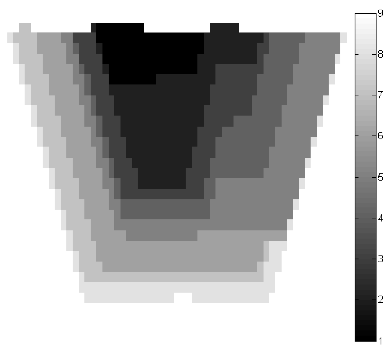Figure 1 presents an East–West section of the production schedule of the study mine as seen from the Figure that slope constraints are properly respected in this proposed study.

The scheduling of the case study presented here is not possible to solve optimally using any commercial solver. Therefore, it is difficult to calculate the optimality gap of our proposed method for the actual mining problem. However, Section 3 has been shown with several problems and comparisons with the upper bound solution. The proposed approach is very close to the upper bound solution with a maximum gap of 4%. Therefore, it can be considered that the generated production schedule for the case study mine is near the optimum solution. Additionally, the total time required for solving the nine years production schedule is 551.4 s; thus, the algorithm is computationally efficient to solve significantly large mine scheduling problems.

After generating the production schedule, the risk profile for mining production is calculated. The minimum, maximum, and average of production from mine are derived from 20 simulations and presented in Figure 2. As observed in Figure 2, the mining capacity in different production periods is within the production limits of the study mine. It is also seen from Figure 2 that the general trend of production is showing an increasing value. This is due to minimizing the penalty of over-production of ore and metal in the initial production periods. The stripping ratio (ore by waste) is also calculated from the production schedule, and it is observed that the stripping ratio is showing a decreasing trend. This result is reasonably expected, similar to other stochastic production schedule models. Therefore, the proposed method is extracting more ores in the initial periods and deferring the waste extraction for the later periods, which eventually increases the cash inflow from the initial mining time.

Similar to mining production, the risk profile for ore processing is calculated from 20 simulations and presented in Figure 3. It is observed from Figure 3 that ore production is maintaining a steady production rate to feed the process plant and achieve the processing capacity. From year 1 to year 8, the average ore production is slightly higher than upper limit target production; whereas, the ore production in the last period is significantly less than the target production limit. The underproduction of ore in the last period is due to the non-availability of enough ore within the remaining pit. The overproduction from year 1 to year eight is penalized; however, those penalties are compensated by revenue generated from those over-productions of ore.

Similar to mining and ore production, the risk profile of metal production is also calculated and presented in Figure 4. The results show that the metals are over-produced in period 1, slightly under-produced from year 2 to year 8, and significantly under-produced in the last period. The over-production in period 1 generates considerably more revenue, thus compensating the penalty due to the over-production. The reason for slightly underproduction from period 2 to period 8 is to minimize the penalty due to the ore production and metal production together. It can be overserved from Figure 3 that ore is over-produced during period 2 to period 8. So, suppose the algorithm tries to produce more metal to stay within the boundary of the metal production target. In that case, it needs to increase the ore production, which eventually introduces more penalties due to the over-production of ore. Therefore, the algorithm optimizes the over-production of ore and under-production of metal so that the mine produces maximum discounted cash flow. Similar to the ore production risk profile, the underproduction of metal in the last period is due to the non-availability of enough metal within the remaining pit of the deposit.

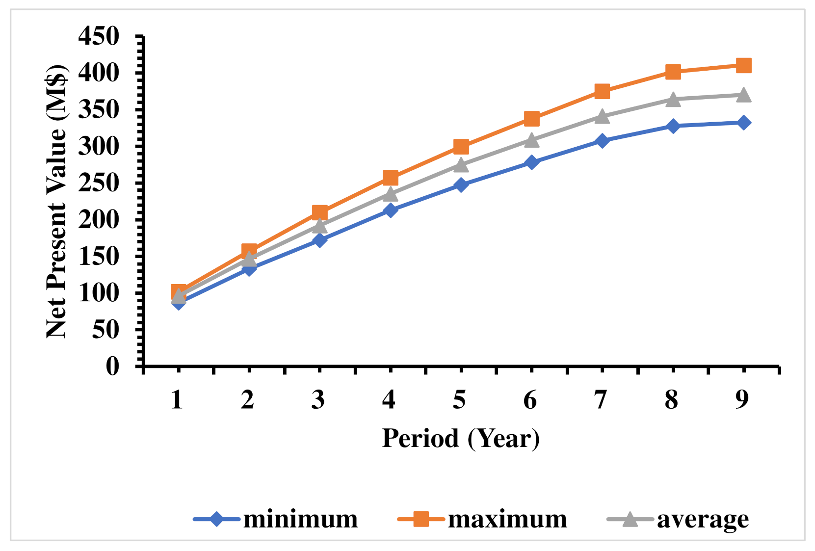
The net present value (NPV) is calculated for determining the risk in the economics. The risk profile using the minimum, maximum and expected NPV is calculated from 20 simulations and presented in Figure 5. The expected NPV generated from the mine is USD 370 million, with a minimum and maximum value of USD 333 million and USD 411 million, respectively. Figure 5 demonstrates that the variability of NPV during the initial period is significantly less compared to the NPV during the later periods. These results reveal that the proposed stochastic model generated revenue with low risk in the initial periods and deferred the risk for the following periods, which are the key benefits of stochastic production scheduling and optimization.

5. Comparison of the Proposed Model with the Sequential Branch-and-Cut Algorithm

In this section, the proposed research is compared with the sequential production schedule generated using the branch-and-cut algorithm. The sequential production scheduling approach is more or less similar to our proposed sequential method; the only difference is that, in this case, the branch-and-cut is directly applied to the formulation of Section 2.2. It is noted that our proposed sequential method used a parametric minimum cut (Section 2.3) and branch-and-cut on the solution from the parametric minimum cut (Section 2.4). The results show that the life of the mine in this approach is nine years, which matches the life of mine using the proposed research approach. The only difference is that all mining blocks (16,532) are extracted over the mine life. It should be noted that the method proposed in this research only removed 15,848 blocks, leaving 684 blocks unmined over the mine life. Figure 6 shows the same East–West Section of the mine production schedule generated using the sequential branch-and-cut approach. When comparing this production schedule with the production schedule created using the proposed research approach, it is observed that the sequence of extractions is different from one another. It is also found that the final pit contour is different in these approaches, and the pit goes dipper in the case of sequential branch-and-cut. The reason is fairly evident as sequential branch-and-cut extracts more mining blocks than the proposed parametric minimum cut with a branch-and-cut approach. When the risk profiles are compared, both the methods show similar trends, except the variability of the risk is not steady in sequential branch-and-cut, unlike the proposed research approach. The cumulative discounted cash follow generated from this study mine using the sequential branch-and-cut algorithm is presented in Figure 7. The risk profile of cash flow also shows a similar behavior as the proposed research approach. The expected NPV generated using this approach is USD 370 million, with a minimum and maximum value of USD 328 million and USD 398 million, respectively. The NPV made from this mine using both the methods are precisely the same; however, it should be noted that the proposed parametric minimum cut with branch-and-cut extracts 3% less amount of mining blocks than sequential branch-and-cut.

When compared to the computational time, it is observed that the sequential branch-and-bound takes 3236 s CPU, which is 5.87 times higher than the parametric minimum cut with the branch-and-cut algorithm. This result demonstrated that the proposed research approach is computationally faster and produce an equally good and better solution (some solutions are better in validation study) than the sequential branch-and-cut algorithm.

6. Comparison between Proposed Stochastic and Deterministic Production Schedule

In this section, the proposed stochastic model is compared with its deterministic counterpart to demonstrate the usefulness of stochastic modeling. The primary purpose of this comparison is to show how the results of the stochastic model improve the production schedule in terms of cash flow generation. The deterministic model is generated using a single estimated orebody model. The estimated orebody model is created by averaging 20 simulated ore bodies. The economic parameters and other mining-related parameters are precisely the same. The solution approach for the deterministic approach is the exact approach used in this paper. Figure 8 shows the section of the production schedule generated using the deterministic orebody model. As expected, the extraction sequence is different in the deterministic model from the stochastic model. It is also interesting to observe that the life of the mine in the deterministic case is ten years, which is higher than the stochastic model. It is also seen from the deterministic production schedule that the number of blocks mined over the mine life is 15,327, which is less than the stochastic model. When comparing the net present values (Figure 9), the deterministic model produces USD 348 million discounted cash flow, which is 6.3% less than the expected value from the stochastic production schedule. Therefore, it can be seen that the stochastic production schedule generates more cash flow over the mine life. The other benefit of the stochastic model is that the risk analysis of all the output parameters can be performed, which eventually gives an insight into the uncertainty associated with the model.

7. Conclusions

In this research, an efficient stochastic mine production scheduling approach is proposed using the parametric minimum cut and branch-and-cut algorithms. The proposed method solved the production schedule sequentially period by period, and at each period, the problem is solved using the parametric minimum cut algorithm. If the solution from the parametric minimum cut algorithm violates the upper limits of the resource constraints, then a repair algorithm is used as the branch-and-cut algorithm to respect those constraints. The proposed method is validated with six relatively small test data sets from copper and iron deposits and compared with the linear relaxation of the original stochastic production scheduling problem. The comparative results demonstrate that the proposed approach is computationally very efficient with low optimality gaps.

The proposed method is applied to a copper data set to show the effectiveness of the approach. The results show that the schedule generated respects the resource constraints with a slight deviation at the initial periods. Moreover, the proposed model uses multiple simulated orebodies for optimizing the production schedule in open pit mines; therefore, it accounts for uncertainty in the model. Furthermore, when comparing with a sequential branch-and-cut approach, it shows that both methods generate similar net present value; however, the computational time of the proposed parametric minimum cut with branch-and-cut is significantly lower than the branch-and-cut algorithm. Finally, the comparison with the deterministic model shows that the proposed approach generates 6% more NPV with a 3% bigger pit size.

The main advantage of the proposed algorithm is that it is computationally very fast; thus, integrating uncertainties in production scheduling is feasible on a routine basis. However, the proposed algorithm cannot provide the true optimal solution due to the sequential solution strategy. Therefore, this algorithm is most suitable for the large mine where the traditional integer programming algorithms take considerable computational time. Moreover, due to the computational speed, the proposed algorithm can quickly provide an excellent initial solution in other optimization models, where reasonable initial solutions are needed. Furthermore, if available, the proposed method can use the updated resource model for the later period of the production schedule due to the sequential approach.

Although the formulation and examples presented here are based on geological uncertainty, the same method can be implemented to incorporate other uncertainties, including demand (commodity price, exchange rate, etc.), cost (mining costs, processing costs, etc.), geometallurgy (hardness, recovery, etc.). Moreover, similar to other production scheduling models, the resource model block size has impact on the final solution of the proposed method due to the dilution and ore losses [44]. The sensitivity of the proposed method on the block size can be an interesting future research.