
Rock Fragmentation Prediction Using an Artificial Neural Network and Support Vector Regression Hybrid Approach


Abstract
:1. Introduction
2. Preliminary Background
2.1. Artificial Neural Network (ANN)
2.2. Suport Vector Regression (SVR)
3. Literature Review
4. Data and Methodology
4.1. Data Source and Description

| ID | S/B | H/B | B/D | T/B | Pf | E (Gpa) | ||
|---|---|---|---|---|---|---|---|---|
| En1 | 1.24 | 1.33 | 27.27 | 0.78 | 0.48 | 0.58 | 60 | 0.37 |
| En2 | 1.24 | 1.33 | 27.27 | 0.78 | 0.48 | 0.58 | 60 | 0.37 |
| En3 | 1.24 | 1.33 | 27.27 | 0.78 | 0.48 | 1.08 | 60 | 0.33 |
| Rc1 | 1.17 | 1.5 | 26.2 | 1.08 | 0.33 | 0.68 | 45 | 0.46 |
| Rc2 | 1.17 | 1.5 | 26.2 | 1.12 | 0.3 | 0.68 | 45 | 0.48 |
| Rc3 | 1.17 | 1.58 | 26.2 | 1.22 | 0.28 | 0.68 | 45 | 0.48 |
| Mg1 | 1 | 2.67 | 27.27 | 0.89 | 0.75 | 0.83 | 50 | 0.23 |
| Mg2 | 1 | 2.67 | 27.27 | 0.89 | 0.75 | 0.78 | 50 | 0.25 |
| Mg3 | 1 | 2.4 | 30.3 | 0.8 | 0.61 | 1.02 | 50 | 0.27 |
| Ru1 | 1.13 | 5 | 39.47 | 1.93 | 0.31 | 2 | 45 | 0.64 |
| Ru2 | 1.2 | 6 | 32.89 | 3.67 | 0.3 | 2 | 45 | 0.54 |
| Ru3 | 1.2 | 6 | 32.89 | 3.7 | 0.3 | 2 | 45 | 0.51 |
| Mr1 | 1.2 | 6 | 32.89 | 0.8 | 0.49 | 1.67 | 32 | 0.17 |
| Mr2 | 1.2 | 6 | 32.89 | 0.8 | 0.51 | 1.67 | 32 | 0.17 |
| Mr3 | 1.2 | 6 | 32.89 | 0.8 | 0.49 | 1.67 | 32 | 0.13 |
| Db1 | 1.25 | 3.5 | 20 | 1.75 | 0.73 | 1 | 9.57 | 0.44 |
| Db2 | 1.25 | 5.1 | 20 | 1.75 | 0.7 | 1 | 9.57 | 0.76 |
| Db3 | 1.38 | 3 | 20 | 1.75 | 0.62 | 1 | 9.57 | 0.35 |
| Sm1 | 1.25 | 2.5 | 28.57 | 0.83 | 0.42 | 0.5 | 13.25 | 0.15 |
| Sm2 | 1.25 | 2.5 | 28.57 | 0.83 | 0.42 | 0.5 | 13.25 | 0.19 |
| Sm3 | 1.25 | 2.5 | 28.57 | 0.83 | 0.42 | 0.5 | 13.25 | 0.23 |
| Ad1 | 1.2 | 4.4 | 28.09 | 1.2 | 0.58 | 0.77 | 16.9 | 0.15 |
| Ad2 | 1.2 | 4.8 | 28.09 | 1.2 | 0.66 | 0.56 | 16.9 | 0.17 |
| Ad3 | 1.2 | 4.8 | 28.09 | 1.2 | 0.72 | 0.29 | 16.9 | 0.14 |
| Oz1 | 1 | 2.83 | 33.71 | 1 | 0.48 | 0.45 | 15 | 0.27 |
| Oz2 | 1.2 | 2.4 | 28.09 | 1 | 0.53 | 0.86 | 15 | 0.14 |
| Oz3 | 1.2 | 2.4 | 28.09 | 1 | 0.53 | 0.44 | 15 | 0.14 |
4.2. Model Development
4.2.1. SVR Modeling
4.2.2. ANN Modeling
5. Results and Discussion
6. Conclusions and Future Work
Author Contributions
Funding
Data Availability Statement
Acknowledgments
Conflicts of Interest
References
- Rustan, A. (Ed.) Rock Blasting Terms and Symbols: A Dictionary of Symbols and Terms in Rock Blasting and Related Areas Like Drilling, Mining and Rock Mechanics; A. A. Balkema: Rotterdam, Holland, 1998. [Google Scholar]
- Cunningham, C.V.B. The Kuz-Ram fragmentation model—20 years on. Bright. Conf. Proc. 2005, 4, 201–210. [Google Scholar] [CrossRef]
- Roy, M.P.; Paswan, R.K.; Sarim, M.D.; Kumar, S.; Jha, R.R.; Singh, P.K. Rock fragmentation by blasting: A review. J. Mines Met. Fuels 2016, 64, 424–431. [Google Scholar]
- Adebola, J.M.; Ogbodo, D.A.; Peter, E.O. Rock fragmentation prediction using Kuz-Ram model. J. Environ. Earth Sci. 2016, 6, 110–115. [Google Scholar]
- Kulatilake, P.H.S.W.; Qiong, W.; Hudaverdi, T.; Kuzu, C. Mean particle size prediction in rock blast fragmentation using neural networks. Eng. Geol. 2010, 114, 298–311. [Google Scholar] [CrossRef]
- Jha, A.; Rajagopal, S.; Sahu, R.; Tukkaraja, P. Detection of geological discontinuities using aerial image analysis and machine learning. In Proceedings of the 46th Annual Conference on Explosives and Blasting Technique, Denver, CO, USA, 26–29 January 2020; ISEE: Cleveland, OH, USA, 2020; pp. 1–11. [Google Scholar]
- Grosan, C.; Abraham, A. Intelligent Systems: A Modern Approach, 1st ed.; Springer: New York, NY, USA, 2011. [Google Scholar] [CrossRef]
- Dumakor-Dupey, N.K.; Sampurna, A.; Jha, A. Advances in blast-induced impact prediction—A review of machine learning applications. Minerals 2021, 11, 601. [Google Scholar] [CrossRef]
- Shi, X.Z.; Zhou, J.; Wu, B.B.; Huang, D.; Wei, W. Support vector machines approach to mean particle size of rock fragmentation due to bench blasting prediction. Trans. Nonferrous Met. Soc. China 2012, 22, 432–441. [Google Scholar] [CrossRef]
- Amoako, R.; Brickey, A. Activity-based respirable dust prediction in underground mines using artificial neural network. In Mine Ventilation–Proceedings of the 18th North American Mine Ventilation Symposium; Tukkaraja, P., Ed.; CRC Press: Boca Raton, FL, USA, 2021; pp. 410–418. [Google Scholar] [CrossRef]
- Ertel, W. Introduction to Artificial Intelligence (Undergraduate Topics in Computer Science), 2nd ed.; Springer: Berlin/Heidelberg, Germany, 2017. [Google Scholar]
- Dixon, D.W.; Ozveren, C.S.; Sapulek, A.T. The application of neural networks to underground methane prediction. In Proceedings of the 7th US Mine Ventilation Symposium, Lexington, KY, USA, 5–7 June 1995; pp. 49–54. [Google Scholar]
- Krose, B.; van der Smagt, P. An Introduction to Neural Networks, 8th ed.; University of Amsterdam: Amsterdam, The Netherlands, 1996. [Google Scholar]
- Zhou, J.; Li, X.; Shi, X. Long-term prediction model of rockburst in underground openings using heuristic algorithms and support vector machines. Saf. Sci. 2012, 50, 629–644. [Google Scholar] [CrossRef]
- Shuvo, M.M.H.; Ahmed, N.; Nouduri, K.; Palaniappan, K. A Hybrid approach for human activity recognition with support vector machine and 1D convolutional neural network. In Proceedings of the 2020 IEEE Applied Imagery Pattern Recognition Workshop (AIPR), Washington, DC, USA, 13–15 October 2020; IEEE: Piscataway, NJ, USA, 2020; pp. 1–5. [Google Scholar]
- Hamed, Y.; Ibrahim Alzahrani, A.; Shafie, A.; Mustaffa, Z.; Che Ismail, M.; Kok Eng, K. Two steps hybrid calibration algorithm of support vector regression and K-nearest neighbors. Alex. Eng. J. 2020, 59, 1181–1190. [Google Scholar] [CrossRef]
- Nandi, S.; Badhe, Y.; Lonari, J.; Sridevi, U.; Rao, B.S.; Tambe, S.S. Hybrid process modeling and optimization strategies integrating neural networks/support vector regression and genetic algorithms: Study of benzene isopropylation on Hbeta catalyst. Chem. Eng. J. 2004, 97, 115–129. [Google Scholar] [CrossRef]
- Gheibie, S.; Aghababaei, H.; Hoseinie, S.H.; Pourrahimian, Y. Modified Kuz-Ram fragmentation model and its use at the Sungun Copper Mine. Int. J. Rock Mech. Min. Sci. 2009, 46, 967–973. [Google Scholar] [CrossRef]
- Kuznetsov, V.M. The mean diameter of the fragments formed by blasting rock. Sov. Min. Sci. 1973, 9, 144–148. [Google Scholar] [CrossRef]
- Cunningham, C.V.B. The Kuz–Ram model for prediction of fragmentation from blasting. In Proceedings of the First International Symposium on Rock Fragmentation by Blasting; Luleå, Sweden, 23–26 August 1983; Holmberg, R., Rustan, A., Eds.; Lulea University of Technology: Luleå, Sweden, 1983; pp. 439–454. [Google Scholar]
- Cunningham, C.V.B. Fragmentation estimations and the Kuz–Ram model—Four years on. In Proceedings of the Second International Symposium on Rock Fragmentation by Blasting, Keystone, CO, USA, 23–26 August 1987; pp. 475–487. [Google Scholar]
- Rosin, P.; Rammler, E. The laws governing the fineness of powdered coal. J. Inst. Fuel 1933, 7, 29–36. [Google Scholar]
- Clark, G.B. Principles of Rock Fragmentation; John Wiley & Sons: New York, NY, USA, 1987. [Google Scholar]
- Kanchibotla, S.S.; Valery, W.; Morrell, S. Modelling fines in blast fragmentation and its impact on crushing and grinding. In Explo ‘99–A Conference on Rock Breaking; The Australasian Institute of Mining and Metallurgy: Kalgoorlie, Australia, 1999; pp. 137–144. [Google Scholar]
- Djordjevic, N. Two-component model of blast fragmentation. In Proceedings of the 6th International Symposium on Rock Fragmentation by Blasting, Johannesburg, South Africa, 8–12 August 1999; pp. 213–219. [Google Scholar]
- Ouchterlony, F. The Swebrec© function: Linking fragmentation by blasting and crushing. Inst. Min. Metall. Trans. Sect. A Min. Technol. 2005, 114, 29–44. [Google Scholar] [CrossRef] [Green Version]
- Hudaverdi, T.; Kulatilake, P.H.S.W.; Kuzu, C. Prediction of blast fragmentation using multivariate analysis procedures. Int. J. Numer. Anal. Methods Geomech. 2010, 35, 1318–1333. [Google Scholar] [CrossRef]
- Ouchterlony, F.; Niklasson, B.; Abrahamsson, S. Fragmentation monitoring of production blasts at Mrica. In Proceedings of the International Symposium on Rock Fragmentation by Blasting, Brisbane, Australia, 26–31 August 1990; McKenzie, C., Ed.; Australasian Institute of Mining and Metallurgy: Carlton, Australia, 1990; pp. 283–289. [Google Scholar]
- Hamdi, E.; Du Mouza, J.; Fleurisson, J.A. Evaluation of the part of blasting energy used for rock mass fragmentation. Fragblast 2001, 5, 180–193. [Google Scholar] [CrossRef]
- Aler, J.; Du Mouza, J.; Arnould, M. Measurement of the fragmentation efficiency of rock mass blasting and its mining applications. Int. J. Rock Mech. Min. Sci. Geomech. 1996, 33, 125–139. [Google Scholar] [CrossRef]
- Hudaverdi, T. The Investigation of the Optimum Parameters in Large Scale Blasting at KBI Black Sea Copper Works—Murgul Open-Pit Mine. Master’s Thesis, Istanbul Technical University, Istanbul, Turkey, 2004. [Google Scholar]
- Ozcelik, Y. Effect of discontinuities on fragment size distribution in open-pit blasting—A case study. Trans. Inst. Min. Metall. Sect. A Min. Ind. 1998, 108, 146–150. [Google Scholar]
- Jhanwar, J.C.; Jethwa, J.L.; Reddy, A.H. Influence of air-deck blasting on fragmentation in jointed rocks in an open-pit manganese mine. Eng. Geol. 2000, 57, 13–29. [Google Scholar] [CrossRef]
- Pedregosa, F.; Varoquaux, G.; Gramfort, A.; Michel, V.; Thirion, B.; Grisel, O.; Blondel, M.; Prettenhofer, P.; Weiss, R.; Dubourg, V.; et al. Scikit-learn: Machine learning in python. J. Mach. Learn. Res. 2011, 12, 2825–2830. [Google Scholar] [CrossRef]
- Chollet, F. Keras. Github Repos. 2015. Available online: https://github.com/fchollet/keras (accessed on 15 June 2020).

| Variable | Minimum | Maximum | Mean | Standard Deviation | |
|---|---|---|---|---|---|
| Input | S/B | 1 | 1.75 | 1.20 | 0.11 |
| H/B | 1.33 | 6.82 | 3.46 | 1.60 | |
| B/D | 17.98 | 39.47 | 27.23 | 4.91 | |
| T/B | 0.5 | 4.67 | 1.27 | 0.69 | |
| Pf (kg/m3) | 0.22 | 1.26 | 0.55 | 0.24 | |
| (m) | 0.29 | 2.35 | 1.16 | 0.48 | |
| E (Gpa) | 9.57 | 60 | 30.18 | 17.52 | |
| Output | (m) | 0.12 | 0.96 | 0.31 | 0.18 |
| Number of Hidden Layers | Optimal Neurons for Hidden Layers | MSE for Test Data | Selected Model |
|---|---|---|---|
| 1 | 90 | 0.0059 | |
| 2 | 25-BN-45 | 0.0039 | |
| 3 | 60-195-190 | 0.0040 | |
| 4 | 115-40-180-35 | 0.0031 | ✓ |
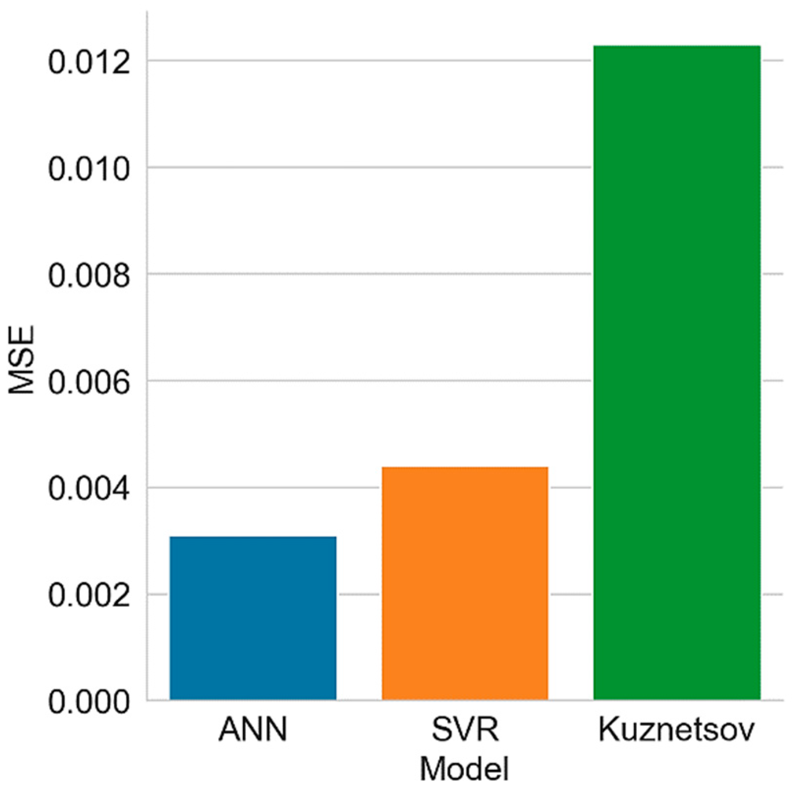
| Model | Mean Squared Error (MSE) | |
|---|---|---|
| Training | Test | |
| = 0.04, kernel = rbf) | 0.0026 | 0.0044 |
| ANN (115-40-180-35) | 0.0028 | 0.0031 |
| Blast Number | Mean Fragment Size (m) | |||
|---|---|---|---|---|
| Actual | Predictions | |||
| ANN | SVR | Kuznetsov | ||
| 1 | 0.47 | 0.44 | 0.38 | 0.48 |
| 2 | 0.64 | 0.68 | 0.64 | 0.71 |
| 3 | 0.44 | 0.38 | 0.41 | 0.42 |
| 4 | 0.25 | 0.25 | 0.25 | 0.33 |
| 5 | 0.20 | 0.15 | 0.14 | 0.27 |
| 6 | 0.35 | 0.21 | 0.52 | 0.09 |
| 7 | 0.18 | 0.19 | 0.19 | 0.38 |
| 8 | 0.23 | 0.17 | 0.18 | 0.22 |
| 9 | 0.17 | 0.17 | 0.19 | 0.25 |
| 10 | 0.21 | 0.21 | 0.20 | 0.12 |
| 11 | 0.20 | 0.21 | 0.19 | 0.13 |
| 12 | 0.17 | 0.24 | 0.26 | 0.23 |
| Coefficient of determination (r2) | 0.87 | 0.81 | 0.58 | |
Publisher’s Note: MDPI stays neutral with regard to jurisdictional claims in published maps and institutional affiliations. |
© 2022 by the authors. Licensee MDPI, Basel, Switzerland. This article is an open access article distributed under the terms and conditions of the Creative Commons Attribution (CC BY) license (https://creativecommons.org/licenses/by/4.0/).
Share and Cite
Amoako, R.; Jha, A.; Zhong, S. Rock Fragmentation Prediction Using an Artificial Neural Network and Support Vector Regression Hybrid Approach. Mining 2022, 2, 233-247. https://doi.org/10.3390/mining2020013
Amoako R, Jha A, Zhong S. Rock Fragmentation Prediction Using an Artificial Neural Network and Support Vector Regression Hybrid Approach. Mining. 2022; 2(2):233-247. https://doi.org/10.3390/mining2020013
Chicago/Turabian StyleAmoako, Richard, Ankit Jha, and Shuo Zhong. 2022. "Rock Fragmentation Prediction Using an Artificial Neural Network and Support Vector Regression Hybrid Approach" Mining 2, no. 2: 233-247. https://doi.org/10.3390/mining2020013
APA StyleAmoako, R., Jha, A., & Zhong, S. (2022). Rock Fragmentation Prediction Using an Artificial Neural Network and Support Vector Regression Hybrid Approach. Mining, 2(2), 233-247. https://doi.org/10.3390/mining2020013