Application of Volume Uncertainty for Resource Classification: A Case Study on the Rondon Do Pará Bauxite Deposit, Brazil

Abstract

This study illustrates the application of conditional simulations to calculate the uncertainty associated with the thickness of bauxite ores. The bauxite deposit of Rondon do Pará in northern Pará State, Brazil, is characterized by a well-defined lateritic profile, with the ore being composed of two sequential horizons: massive bauxite and ferruginous bauxite. This study used ore thickness data from 1.005 drillholes with different grid spacing. Drillhole intervals of both types of bauxite ore were accumulated, converting the database from 3D to 2D. Sequential Gaussian simulation produced probability maps calculated from certain confidence intervals, which permits obtaining the uncertainty associated with estimates in thickness. Results show that in portions with the same regular drillhole spacing there are different ranges of uncertainty and variability, which could be useful to support resource classification, associating different confidence intervals to resource classes. This analysis could also guide the drilling program for resource conversion in order to optimize costs, indicating areas where there is greater uncertainty and would need to be densified. The incorporation of this information into the resource model could be very helpful for supporting subsequent studies of economic evaluation and risk analyses with respect to this type of deposit or similarly in mineral exploration.

1. Introduction

Over the last decade, the mineral industry demanded a higher level of confidence in reported mineral resources for both development projects and mines in production. Studies showing conditional simulation techniques supporting resource classification are frequent [1,2,3,4]. However, this technique is commonly applied to grade data [5,6], and volume uncertainty is less commonly calculated.

An example of a discussion about different geological interpretations that directly reflect on the volume variation can be observed in Jackson et al. [7]. Nevertheless, in stratigraphic deposits, such as bauxite deposits, geological interpretation is not critical. Stratigraphic deposits comprise roughly flat surfaces and appear conformably on top of underlying older volumes, and their contacts do not cut across other contacts in the geological sequence. Bauxite ore bodies have extensive lateral continuity and variability in volume and, consequently, in tonnage; this is a direct function of ore-layer thickness. In this type of deposit, thickness variabilities are much more significant than the variability in the alumina’s content. Thickness uncertainty has been quantified for the lateritic bauxite deposit of Rondon in northern Pará State, Brazil. This provides a simple method for assessing volume uncertainty using thickness data.

This paper expands discussions on the results originally presented in a conference paper by de Oliveira et al. [8]. The text is organized to present the geology of the deposit, the methodology used to calculate uncertainty, and finally, the results are provided as maps of probability, which are discussed and interpreted to support mineral resource classification.

2. Case Study

Rondon Do Pará Bauxite Deposit

The bauxite deposit of Rondon do Pará is located in the city of Rondon do Pará, Pará State, along with other world-class Amazon bauxite deposits in northern Brazil [9] (Figure 1).

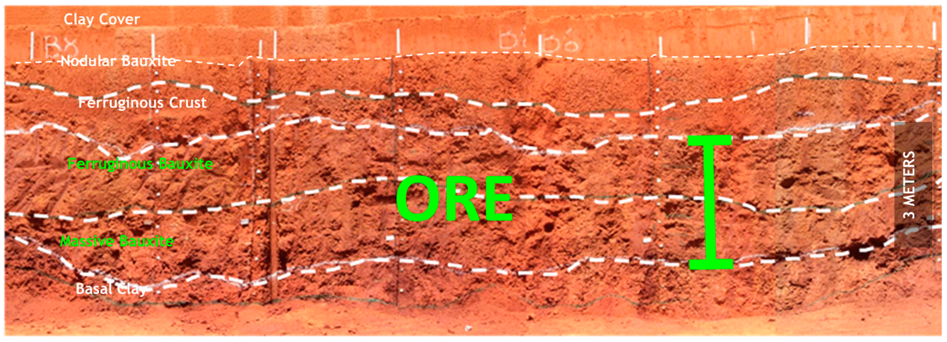
The Rondon do Pará is a large deposit with many plateaus over 20 km of extension surface. The deposit shows a well-defined bauxite-bearing lateritic profile comprising five horizons from the bottom to the top: basal clay, massive bauxite, ferruginous bauxite, ferruginous crust, and nodular bauxite, followed by a clay cover (Figure 2) [9,10,11]. Of these, massive bauxite and ferruginous bauxite horizons are considered as ores, and they are differentiated by variations in Fe₂O₃ and Al₂O₃ content [9]. This is a typical horizontal deposit with very well-defined layers that do not cross themselves.

The map in Figure 3 shows the distribution of drillholes in the deposit. The drillholes are located in regular grids with different spacing ranging from 200 m to 1600 m. A higher density of drillholes is concentrated in the southwestern portion of the deposit, where the greatest thickness of the ore in the deposit occurs (Figure 3).

The dataset comprised 1005 vertical drillholes that intersect bauxite ore. As all ore layers of the deposit are horizontal and it does not have any faulting or deformation, the intersecting length is the real thickness of the orebody.

3. Materials and Methods

The study was developed with all drillholes in the entire plateau in the GSLIB platform [12]. The average length of the samples is 0.5 m, and the layer of bauxite ore occurs at an average of 1.50 m. Commonly, there is more than one sample per drillhole for the ore layer. Therefore, sample lengths were summed by generating a single value per drillhole, thus enabling work in 2D. The step-by-step workflow from the accumulation of drillhole intervals to the 3D to 2D database conversion is illustrated in Figure 4.

The variability in thickness was quantified by stochastic conditional simulations. The algorithm used was Sequential Gaussian [13]. Sequential Gaussian simulations are one of the most widely applied simulation algorithms used to understand heterogeneities and to quantify the uncertainty of regionalized variables. Sequential simulations correctly reproduce the distribution and covariance of the original data. As thickness data are non-Gaussian, they were initially transformed to a Gaussian variable using a quantile transform, the simulations were performed, and finally, data are backtransformed to the original distribution [14]. The sequential simulation principle [13] is based on the factorization of the joint probability, P, of a set of m random variables (RV), Y, and n conditioning data. The set of m RVs could represent the nodes of a grid that discretizes the domain to a model. The grid was generated with regular blocks of 100 × 100 m. The resource classification follows the proposal of Snowden [15], with each block being classified according to a confidence level.

4. Results

4.1. Data Analysis

As the distribution of data is irregular throughout the domain of interest, declustering analyses are necessary. This technique assigns a weight based on the spacing between each sample. The declustering method used was cell declustering [16]. Figure 5 shows the variation of the average over windows with different cell sizes. The average tends to stabilize close to 100 m thick after the 6000 m cell size. This cell size is selected as the optimal size.

The distribution of original thickness data by histogram and the cumulative curve is shown in Figure 6. The average of the samples drops to 1.08 m instead of 1.58 m in the clustered data.

4.2. Ordinary Kriging

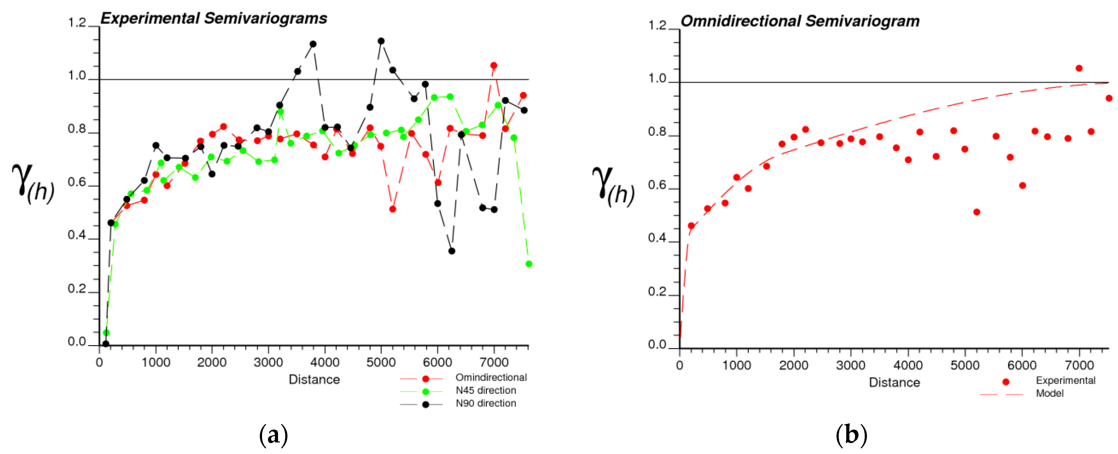
Ordinary kriging estimations were performed to assess the spatial variability of deposit thicknesses considering an omnidirectional variogram (Figure 7). The variogram of the data is a spherical model with a range of 200 m. Figure 8 shows the ordinary kriging map.

Nugget effects were not considered, as they are not expected with the large variability in microscale for thickness values. The variogram range may be even greater than 6500 m given the vast extent of the bauxite ore layer in the deposit. However, because we are more interested in the pattern of the variogram near the origin, the adjustment to the variance was performed in a 200 m range. Below is the variogram model in Figure 7b.

γ (h): 0.32 Sph (200) + 0.15 Sph (6500)

4.3. Sequential Gaussian Simulation

Sequential Gaussian simulation was used to assess the uncertainty in thickness data. Declustered data were initially transformed to generate a normal distribution. Variograms were calculated for the transformed variables. Normal score variograms are very similar to those calculated for the original data (Figure 9). The conditional simulation was performed using simple kriging, performing 100 simulations. Figure 10 shows the first four simulations obtained.

Realizations of the original data and the variogram are plotted together to validate the estimations (Figure 11). The conditional simulation reproduces the data distribution and the variogram of the original data in all 100 realizations. In general, the results are good and reproduce the input statistics.

Additionally, relative to the initial checks, an accuracy plot is presented in Figure 12, which shows values that are in a certain range plotted against the probability of being within this range, following the methodology of Deutsch [17]. The closer the line, the more precision and accuracy it has. The scatterplot shows very good results, with high accuracy and precision in the simulation (Figure 12).

4.4. Backtransformation

To work with the same data units, it is necessary to backtransform Gaussian-simulated data. Figure 13 shows the same four realizations of Figure 10 backtransformed in the original units. In general, the realizations reasonably reproduce the spatial distribution of values if compared to ordinary kriging maps (Figure 8).

4.5. Post Processing

Probability maps were calculated from certain thresholds to obtain the uncertainty associated with estimates in thickness. A visual analysis of maps with different cutoffs of thickness data ranging from 1.00 m to 3.00 m is shown in Figure 14.

Another method for analyzing the deposit is by filtering realizations that have average values above a certain cutoff. Figure 15 shows the map with thickness values greater than 1.00 m.

Conditional simulation results also allow the classification of domains of the deposit according to a confidence interval. Figure 16 shows the results for intervals of 90%, 85%, 80%, and 75%.

Few blocks have high probabilities for a confidence interval of 90%. However, even in portions where the drillhole spacing is larger, there are different probabilities for the same confidence interval.

The proposed classification could be flagged into blocks through a contour line generated around the portions of the deposit that predominates the threshold values (Figure 17).

Table 1. Resource classification based on the probability for confidence intervals.

Category	Confidence Level
Measured	0–10%
Indicated	10–20%
Inferred	>20%

lists the categories of mineral resources according to the JORC [18] nomenclature with selected probability intervals [15].

5. Discussion

Drill spacing is one of the main criteria widely used in resource classification today [4], both in mines in production and exploration projects. However, quantitative methods of uncertainty assessment of geological models are not yet routinely used in the classification and evaluation of mineral resources [19].

Figure 17 shows that within a domain defined only by the drilling spacing criterion (black line) different levels of uncertainty are found. These uncertainties are related to the inherent natural geological variability of the deposit, classified as stochasticity and inherent randomness by Mann [20], Bárdossy and Fodor [21], and Wellmann et al. [22].

However, at first glance, the confidence interval approach shows that an area and consequently a smaller volume has been classified as a Measured resource, requiring a higher cost with additional drilling. In fact, this approach could indicate zones within the deposit where resources are classified as Inferred and Indicated and drilling spacing could only be densified, converting them into Indicated and Measured resources, respectively, thus optimizing drilling costs. Thus, in Figure 17, in the domain defined within the purple line, mineral resources would be classified as Measured, and no further drilling would be necessary. In the domains within the black line but outside the purple line, additional drilling would be required for resource conversion according to a respective confidence interval.

The presented methodology proposes a simple method for adding the uncertainties associated with the deposit tonnage to the classification of resources. Most techniques found in the literature focus on parameters based on grade estimation and leave aside the uncertainty related to volume and, consequently, tonnage. The idea is to use volume uncertainty to assist in resource classification.

The main advantage of applying this methodology is to obtain a numerical value for uncertainty, whereas many classification approaches use subjective uncertainty assessments.

An important observation in this study is that different regions of the deposit with the same regular drillhole spacing, show different variability. This implies that techniques based on drill hole spacing and search neighborhoods would require local customization.

The 2D methodology presented here would have greater applicability in extensive stratiform and stratigraphic deposits such as iron, coal, phosphate, and lateritic types. Base metal and precious metal deposits usually have different drillhole spacing and direction, and the intersections do not necessarily reflect the true thickness; 3D complexity would be better handled by 3D modeling and not thickness mapping.

6. Conclusions

Applying Gaussian simulations in evaluating mineral deposits was shown to be an interesting tool, allowing the assessment of uncertainty and adding this information to the resource model.

Results for the bauxite deposit of Rondon do Pará show that in portions with the same drilling spacing, there are different ranges of uncertainty and variability, which could be useful in supporting resource classification, associating different confidence intervals to resource classes. This analysis can also guide the drilling program for resource conversion in order to optimize costs, indicating areas in which there is greater uncertainty and areas that would need to be densified, while areas with less uncertainty would not require extra drilling.

The incorporation of this information into the resource model could be very useful for supporting subsequent studies of economic evaluation and risk analyses in this type of deposit or similarly in mineral exploration.

References

- Annels, A.E. Mineral Deposit Evaluation: A Practical Approach; Springer: Dordrecht, The Netherlands, 1991. [Google Scholar]
- Mwasinga, P.P. Approaching resource classification: General practices and the integration of geostatistics. In Computer Applications in the Mineral Industries; Xie, H., Wang, Y., Jiang, Y., Eds.; CRC Press: Boca Raton, FL, USA, 2001; pp. 97–104. [Google Scholar]
- Sinclair, A.J.; Blackwell, G.H. Applied Mineral Inventory Estimation; Cambridge University Press: Cambridge, UK, 2002. [Google Scholar]
- Silva, D.S.F.; Boisvert, J.B. Mineral resource classification: A comparison of new and existing techniques. J. South. Afr. Inst. Min. Metall. 2014, 114, 265–273. [Google Scholar]
- Souza, L.E.; Costa, J.F.C.L.; Koppe, J.C. Comparative analysis of the resource classification techniques: Case study of the Conceição mine, Brazil. Appl. Earth Sci. 2010, 119, 166–175. [Google Scholar] [CrossRef]
- Emery, X.; Ortiz, J.M.; Rodríguez, J.J. Quantifying uncertainty in mineral resources by use of classification schemes and conditional simulations. Math. Geol. 2006, 38, 445–464. [Google Scholar] [CrossRef]
- Jackson, S.; Frederickson, D.; Stewart, M.; Vann, J.; Burke, A.; Dugdale, J.; Bertoli, O. Geological and Grade Risk at the Golden Gift and Magdala Gold Deposits, Stawell, Victoria, Australia. In Proceedings of the Fifth International Mining Geology Conference, Bendigo, Australia, 7–19 November 2003; Australasian Institute of Mining and Metallurg: Carlton, Australia; pp. 207–214. [Google Scholar]
- de Oliveira, S.B.; Boisvert, J.B.; Deutsch, C.V. Assessment of thickness uncertainty using geostatistical simulation in the Rondon do Pará bauxite deposit, Brazil. In Proceedings of the 37th APCOM, Fairbanks, AK, USA, 23–27 May 2015; p. 13. [Google Scholar]
- de Oliveira, S.B.; da Costa, M.L.; dos Prazeres Filho, H.J. The lateritic bauxite deposit of Rondon do Pará: A new giant deposit in the Amazon region, Northern Brazil. Econ. Geol. 2016, 111, 1277–1290. [Google Scholar] [CrossRef]
- Santos, P.H.C.d.; Costa, M.L.d. Mineralogy, geochemistry and parent rock of Décio bauxite-bearing lateritic profile (Rondon do Pará, Eastern Amazon). Braz. J. Geol. 2022, 51. [Google Scholar] [CrossRef]
- Negrão, L.B.A.; Costa, M.L.d.; Pöllmann, H. The belterra clay on the bauxite deposits of Rondon do Pará, Eastern Amazon. Braz. J. Geol. 2018, 48, 473–484. [Google Scholar] [CrossRef]
- Deutsch, C.V.; Journel, A.G. Gslib Geostatistical Software Library and User’s Guide, 2nd ed.; Oxford University Press: Oxford, UK, 1998. [Google Scholar]
- Isaaks, E.H. The Application of Monte Carlo Methods to the Analysis of Spatially Correlated Data. Ph.D. Thesis, Stanford University, Stanford, CA, USA, 1991. [Google Scholar]
- Chiles, J.P.; Delfiner, P. Geostatistics: Modeling Spatial Uncertainty, 2nd ed.; Wiley Interscience: New York, NY, USA, 2012. [Google Scholar]
- Snowden, D.V. Practical interpretation of mineral resource and ore reserve classification guidelines. In Mineral Resource and Ore Reserve Estimation—The Ausimm Guide to Good Practice; Edwards, A.C., Ed.; Australasian Intitute of Mining and Metallurgy Melbourne: Melbourne, Australia, 2001; pp. 643–652. [Google Scholar]
- Deutsch, C. Declus: A fortran 77 program for determining optimum spatial declustering weights. Comput. Geosci. 1989, 15, 325–332. [Google Scholar] [CrossRef]
- Deutsch, C.V. Direct assessment of local accuracy and precision. Geostat. Wollongong 1997, 96, 115–125. [Google Scholar]
- JORC. The Jorc Code-2012 Edition: Australasian Code for Reporting of Exploration Results, Mineral Resources and Ore Reserves; Australasian Intitute of Mining and Metallurgy Melbourne: Melbourne, Australia, 2012; p. 44. [Google Scholar]
- McManus, S.; Rahman, A.; Coombes, J.; Horta, A. Uncertainty assessment of spatial domain models in early stage mining projects—A review. Ore Geol. Rev. 2021, 133, 104098. [Google Scholar] [CrossRef]
- Mann, J.C. Uncertainty in geology. In Computers in Geology—25 Years of Progress; Oxford University Press: Oxford, UK, 1993; pp. 241–254. [Google Scholar]
- Bárdossy, G.; Fodor, J. Traditional and new ways to handle uncertainty in geology. Nat. Resour. Res. 2001, 10, 179–187. [Google Scholar] [CrossRef]
- Wellmann, J.F.; Horowitz, F.G.; Schill, E.; Regenauer-Lieb, K. Towards incorporating uncertainty of structural data in 3d geological inversion. Tectonophysics 2010, 490, 141–151. [Google Scholar] [CrossRef]
Figure 1.
Geologic map with the location of the Rondon do Pará deposit along with other world-class Amazon bauxite deposits (after de Oliveira et al. [
9]).
Figure 2.
Trench photo showing the lateritic profile in the Rondon do Pará bauxite deposit.
Figure 3.
Location of drillholes with thickness data.
Figure 4.
Step-by-step workflow for (A) selecting ore thickness intervals, (B) accumulating these intervals, and (C) converting 3D databases (intervals) to 2D (points).
Figure 5.
Scatterplot of declustered means by cell size (meters) of moving window.
Figure 6.
Distribution of thickness: (a) clustered data and (b) declustered data.
Figure 7.
(a) Experimental variograms in the directions N45, N90, and omnidirectional and the (b) adjusted model for the omnidirectional variogram.
Figure 8.
Thickness model estimated by ordinary kriging.
Figure 9.
(a) Experimental variograms for normal score variable in the directions N45, N90, and omnidirectional and (b) the adjusted model for the omnidirectional variogram.
Figure 10.
First four realizations in normal score units.
Figure 11.
(a) Cumulative curve for 100 realizations compared to the original data and (b) variograms for 20 realizations compared to the original data.
Figure 12.
Accuracy check of the outputs.
Figure 13.
First four realizations on original units.
Figure 14.
Probability maps with cutoffs of 1.00, 1.50, 2.00, and 3.00 m.
Figure 15.
Map with average thickness greater than 1.00 m.
Figure 16.
Maps of probability for confidence intervals of 90%, 85%, 80%, and 75%.
Figure 17.
Map of probability for confidence intervals of 85% with a black contour line for a drillhole spacing-based approach (200 m) and a purple contour line for an uncertainty-based approach.