Comparison of MLR, MNLR, and ANN Models for Estimation of Young’s Modulus (E₅₀) and Poisson’s Ratio (υ) of Rock Materials Using Non-Destructive Measurement Methods

Abstract

In this study, the static E₅₀ and υ parameters of rock materials were investigated using P-S wave velocities and Shore hardness (SH), using non-destructive measurement methods. In this study, the multiple linear regression (MLR), multiple non-linear regression (MNLR), and artificial neural network (ANN) models were used to estimate and determine the static E₅₀ and υ parameters. When comparing the models defined by MLR, MNLR, and ANN to the R² values, it was found that the ANN models, which estimate the E₅₀ and υ parameters of rock materials using non-destructive methods (V_p, V_s, V_p/V_s, ρ_d, and SH), achieved higher accuracy than the MLR and MNLR models. The originality of this study is rooted in the fact that ores such as galena, chromite, and barite were studied for the first time from a rock mechanics perspective, providing an innovative viewpoint. In addition, the use of all non-destructive measurement methods, V_p, V_s, and Shore hardness tests, also increases the importance of the study findings.

1. Introduction

Determining the physicomechanical parameters of rock materials can be accomplished using two methods: destructive and non-destructive. While destructive methods include tests such as the uniaxial compressive strength (UCS), triaxial compressive strength (TCS), and direct (TS) and indirect tensile strength (ITS), non-destructive methods include experimental tests such as seismic wave velocities, and Schmidt and Shore hardnesses. The measurement of the physicomechanical properties of rocks has been conducted based on both the ISRM (1981) [1] and the ASTM (1984) [2] standards. Destructive measurement methods are generally conducted in the laboratory using specific test equipment that contains the core specimens. Moreover, in destructive measurement methods, when rock materials are generally weak, thin-bedded, or heavily fractured, they may not be suitable for the sample preparation and measurements required for mechanical tests. On the other hand, non-destructive measurement methods are based on the measurement of seismic velocities or the hardness of the rock, sometimes in situ but usually in the laboratory [3,4,5,6]. Additionally, non-destructive tests are easier because they require less sample preparation, and the test equipment is simple to use. They can also be easily used on the mine site. Therefore, non-destructive measurement methods are faster, simpler, and more economical than destructive measurement methods.

Hardness is one of the physical properties of materials, and the Schmidt and Shore hardness (SH) measurements are the best-known methods for rock materials. While very large rock masses are required for the Schmidt hardness measurement, smaller rock pieces can also be measured for the Shore hardness measurements. In addition, SH is widely used to estimate the hardness of rock materials because it is an easy-to-use and inexpensive method. Similarly, the seismic velocities (V_p and V_s) of rock materials are easy and simple to measure and values are calculated according to the cleavage, crystalline structure, fracture structure, elasticity, porosity, and density properties that define the physicomechanical properties of the rock materials.

Two of the most important physicomechanical parameters of rock materials are the E₅₀ and υ. These parameters are very important in tunnel design, rock blasting and drilling, slope stability, pillar design, and many construction and mining activities. These parameters are also used to express the resistance of materials to deformation under shear or compressive stresses. The E₅₀ and υ are affected by many factors such as the crystalline structure of the rock material, cleavage, crack structure, elasticity, anisotropy state, and mineralogical composition [7,8].

One of the engineering problems related to rock materials stems from the incorrect evaluation of their physicomechanical properties. First of all, high-quality core samples are required to determine the E₅₀ and υ parameters. However, sometimes it is not easy to obtain smooth cores, especially from very fractured, weak, or very hard rock materials [9,10,11]. Moreover, even if high-quality cores can be obtained to perform tests such as UCS, TS, and ITS, it is a costly, laborious, and time-consuming process in terms of human errors, instrument calibration issues, and internal factors. Therefore, engineers often estimate E₅₀ and υ parameters from other static and dynamic rock parameters by using the estimation equations published in the literature for their required projects. Of course, the accuracy of these estimation equations is debatable.

2. Previous Studies

Researchers [3,12,13,14,15,16,17,18] have conducted numerous studies on estimating the E₅₀ and υ using other static tests such as UCS, ITS, Schmidt hardness, and rock mass rating (RMR₈₉) [17] for various rock material types. These researchers [3,10,11,12,13,14,15,16,17,18] have developed many simple linear or simple non-linear equations for estimating the E₅₀ or υ values. However, most of the equations are not suitable for all types of rock environments when estimating these parameters (E₅₀ and υ), and those suitable tend to provide accurate results only for specific rock types, such as the sedimentary or metamorphic groups. Sonmez et al. (2006) [19] estimated the E₅₀ value using the ANN model with the UCS and the unit weight (γ) for different types of intact rocks. However, obtaining the UCS and γ values are far from being an alternative for estimating the E₅₀ values, as the sample preparation and testing process is as tedious and difficult as obtaining the E₅₀ values themselves. Meanwhile, other researchers [9,20,21] have tried to estimate the E₅₀ and υ with the Shore hardness (SH) test with simple linear or simple non-linear regressions, but the relationships were revealed to have a low correlation. Karakus et al. (2005) [22] proposed a good model with a high R² value (0.982) using the MLR model to estimate the E₅₀ and υ based on the findings from some rock mechanic experiments. However, the use of point load index (I_s) and uniaxial compressive strength (UCS) tests in the model is far from being an alternative method as the preparation of the core samples for these tests is onerous.

Other researchers [4,7,20,23,24,25,26,27,28] have also investigated the relationships between the non-destructive measurement tests and the static physicomechanical parameters (destructive measurements) for the same type of rock materials at a mining site, or for specific groups of rock materials such as those of sedimentary or metamorphic origins. When the results of the research were examined, it was shown that there were significant correlations between the seismic velocities, especially the V_p velocity, of rock samples taken from a similar particular group or region. Armaghani et al. (2016) [8] further investigated the estimation of E₅₀ from the V_p, porosity (n), Schmidt hardness (R_n), and point load strength (I_s(50)) values for granite samples using the MLR and ANN models. They not only found MLR and ANN models with very low coefficients of determination (R² = 0.643 and 0.596, respectively), but also used laborious and difficult methods to determine the properties of the materials such as the porosity and the point load strength in the models.

As can be seen from the previous studies, although many testing methods are widely used in the estimation of the physicomechanical parameters of rock materials, there is limited research on the use of non-destructive measurement methods for estimating the E₅₀ and υ values of rock materials. Moreover, the determinant coefficients (R²) for the estimation models were low and the error values (RMSE and MAE, etc.) were high. Therefore, it is inevitable that the development of the models for estimating the parameters with easier, less laborious, less time-consuming, cheaper, and higher accuracy methods will continue to be an important research topic for many researchers.

Artificial neural networks (ANNs) have attracted great attention in recent years for the estimation of various physicomechanical parameters such as UCS, ITS, shear strength parameters, and the modulus of various rock materials [8,19,29,30,31,32,33,34,35]. The reason that ANN has become especially popular is that it allows for more flexible operations between variables with a greater number of input variables, overcoming the low coefficients of determination obtained from regression analyses such as MLR and MNLR. Therefore, ANN has a great capability for modeling the physicomechanical behavior of rock materials [29] and has been shown by many researchers to provide more accurate estimates of the physicomechanical parameters of rock materials than the other statistical models. Some researchers [8,30,31,32,33,34,35,36] have shown that ANNs provide much more realistic estimations than the other statistical models for estimating the physicomechanical parameters of rock materials. In this context, this study aimed to determine the static E₅₀ and υ parameters of rock materials using non-destructive measurement methods (V_p, V_s, and SH) through MLR, NMLR, and ANN models.

3. Materials and Methods

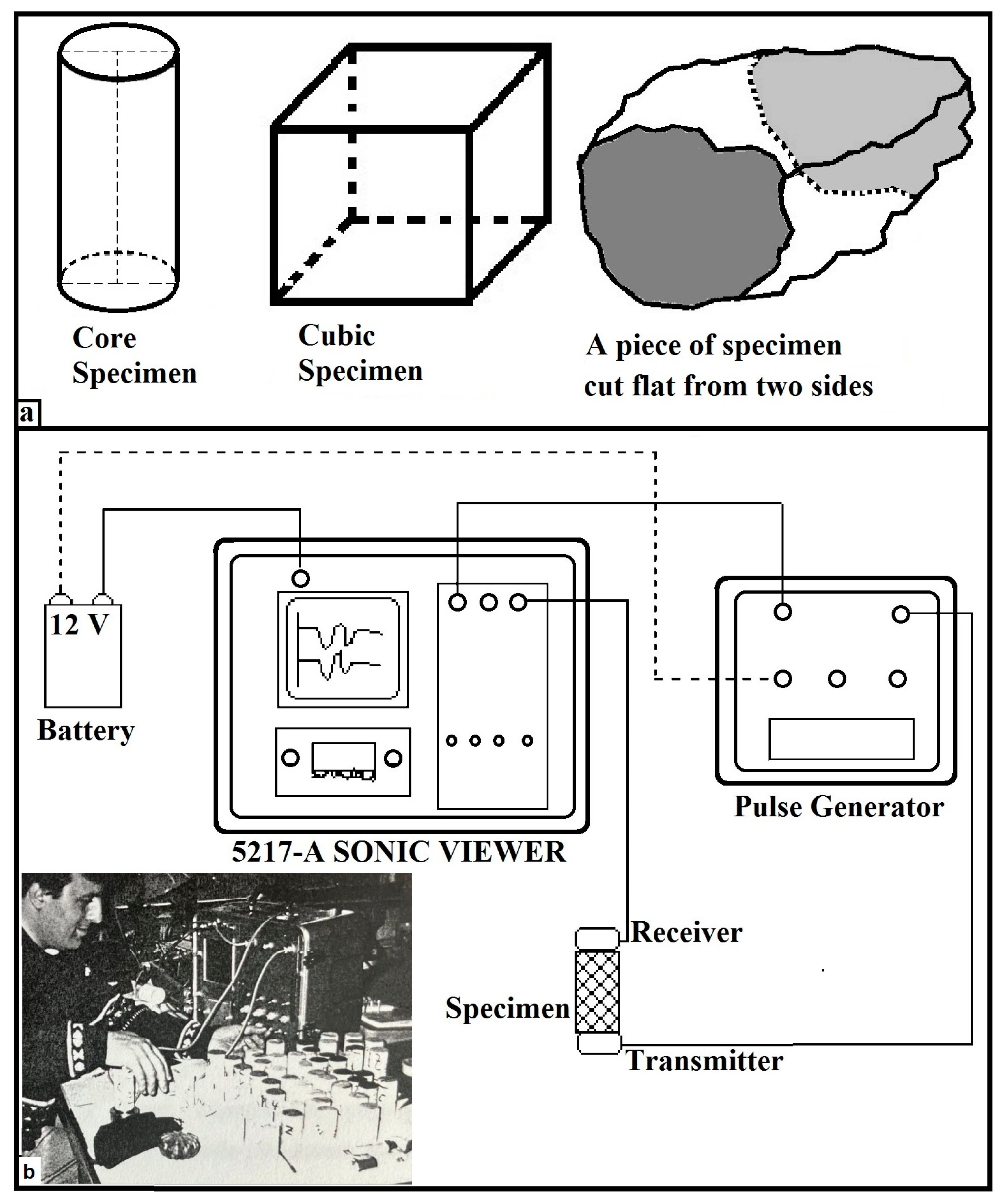
In this study, non-destructive measurement models were developed to estimate the E₅₀ and υ of rock materials by using the properties of ultrasonic wave velocities (V_p and V_s), dynamic density (ρ_d), and Shore hardness (SH) values. These non-destructive measurement methods do not require special specimen preparation requirements such as coring and large specimen sizes. Also, they are much easier to use compared to the stress-strain tests used to obtain E₅₀ and υ values. These non-destructive tests can be used to estimate rather than measure the E₅₀ and υ values. The main advantages of non-destructive measurement methods are their ease of use and flexibility.

This study aims to estimate the E₅₀ and υ obtained using stress-strain curves under compression from non-destructive measurement methods (V_p, V_s, V_p/V_s, ρ_d, and SH) using the MLR, MNLR, and ANN models. A series of analyses were performed on a total of 17 rock types of different geological origin, including sedimentary (8), metamorphic (2), igneous-volcanic (4), and mafic-ultramafic igneous ores (3). This study will be the first study on a very different sample group, including mafic and ultramafic igneous ores such as sulfide ore, galena, and chromite. In this respect, it will be an important contribution to the literature.

3.1. Materials

A total of 17 different rock types were collected from various regions in Turkey. At least nine samples were taken from each rock type, at least 3 in the X-Y-Z direction. The mineralogical properties of the rock types used in the tests are presented in

Table 1. The materials used for the tests along with their mineralogical properties.

No.	Description	Geological Origin	Mineralogical Properties
1	Limestone-1	Sedimentary	50% clay content
2	Limestone-2	Sedimentary	very low porosity, sandy limestone texture
3	Limestone-3	Sedimentary	micritic texture, fracture filling calcite, and contains a small amount of opaque minerals
4	Limestone-4	Sedimentary	sparitic and homogenously textured
5	Siltstone	Sedimentary	contains 60% quartz
6	Green-Marl	Sedimentary	contains a small amount of silica
7	Gypsum	Sedimentary	less opaque and subhedral minerals
8	Barite	Sedimentary	15% anhedral particle, may be subject to tectonism, a hydrothermally deposited ore
9	Feldspar	Metamorphic	coarse crystalline albite mineral, contains 50% quartz minerals
10	Marble	Metamorphic	contains equidimensional and anhedral calcite crystals
11	Trass-1	Igneous-Volcanic	contains amphibole, sanidine, and biotite
12	Trass-2	Igneous-Volcanic	contains 50% quartz minerals
13	Andesite-1	Igneous-Volcanic	porphyritic, altered
14	Andesite-2	Igneous-Volcanic	porphyritic, less altered
15	Galena	Mafic/Ultramafic-Igneous ore	also contains pyrite and chalcopyrite
16	Sulfide ore	Mafic/Ultramafic-Igneous ore	contains galena, pyrite, chalcopyrite, and quartz
17	Chromite	Mafic/Ultramafic-Igneous ore	contains 80% chromite, olivine, and serpentine

.

As shown in Figure 1a–d, the core samples of 54 mm diameter were prepared from the collected rock masses in the laboratory. In the non-destructive experimental studies, V_p and V_s were first measured in the core specimens with a sonic wave viewer, and then Shore hardness (SH) was measured in the same core specimens with a Shore Scleroscope C-2 (as seen in Figure 1g).

In the destructive experimental studies, according to the test procedures recommended by ASTM D7012-14e1 (2017) [37], stress-strain measurements were performed on core specimens under compression, as shown in Figure 1e,f. The static E₅₀ and υ values were calculated from the stress-strain curves which were simultaneously recorded using a computer. After the destructive and non-destructive tests, statistical modeling studies were started. While the V_p and V_s wave velocities (m/s), V_p/V_s ratios, dynamic densities (ρ_d, t/m³), and Shore hardness (SH) values were also used as input data in the modeling, the E₅₀ and υ values were then considered as output data.

3.2. Sonic Wave Velocity (V_p and V_s) Tests

In this study, sonic wave velocity measurements (V_p and V_s) were applied according to the ASTM D2845-08 (2008) [38] standards. For the measurement of V_s and V_p, specimens should be cylindrical (core) or cubical or cut straight so that both sides of the specimen are parallel (Figure 2a). The easiest among these is to cut the samples neatly from both sides. For this, samples can be cut on a rock-cutting machine. In our study, sonic velocity tests were performed on a total of 10–15 core specimens taken from three directions (3–5 cores from each direction) to determine the static E₅₀ and υ values, taking into account the anisotropic condition of each rock block sample.

The OYO sonic viewer (OYO Corporation, Tokyo, Japan) (Model 5217-A), which includes a battery, a receiver, a transmitter, an ultrasonic pulse generator, and a signal data acquisition and display system (as shown in Figure 2b), was used to measure the ultrasonic wave velocities (V_p and V_s) of the rock materials. Before measuring the ultrasonic wave velocity, the ends of the core specimens were first polished, and a thin layer of grease was then applied. The ultrasonic wave (V_p and V_s) velocities are calculated using the travel time of the measured wave and the distance between the transmitter and the receiver, i.e., the measured sample length.

The specific density value of a rock material is an important factor in engineering studies. The density of the rock material was determined directly (destructive method) by measuring, as well as indirectly (non-destructive method) by calculating. The specific density can be determined using Archimedes’ principle in the laboratory. This is a time-consuming and tedious process. For this reason, many researchers have been working to determine the specific density value indirectly using seismic wave velocities (V_p and V_s) since the 1970s. Telford et al. (1976) [39] investigated the relationship between the specific density of rock materials and the seismic wave velocities. They stated that the dynamic density of rock materials can be found from the P-wave velocity (V_p), using Equation (1).

ρ_d = 0.2V_p + 1.6

(1)

3.3. Shore Hardness Tests

The Shore hardness instrument is a non-destructive measuring instrument for use on relatively small specimens and measures the relative values of Shore hardness (SH) with a diamond-tipped hammer which falls freely from top to bottom onto a smooth specimen [40]. The ISRM (1981) [41] has proposed a method using the C-2 model Shore hardness instrument for rock materials.

Specimens can also be created for SH measurements like the ultrasonic wave velocity measurements by obtaining cylindrical (core) or cubic specimens from the rock blocks or by smoothly cutting from both sides of the rock specimen. The method of smooth cutting from both sides of the rock specimens has become an easy method for determining SH, especially if the specimens are small in size (a minimum surface area of 10 cm² and a minimum thickness of 10 mm) or cannot be cored [38]. In this study, Shore hardness measurements were also carried out after the ultrasonic wave velocity tests were performed on the core samples. Shore hardness measurements were accepted as the SH of the rock material after calculating the arithmetic average of approximately 200 readings from ~10 cores, with at least 20 readings from each core specimen.

3.4. The Stress-Strain Tests to Determine E₅₀ and υ Values

In this study, cylindrical specimens (cores of 108 mm length and 54 mm diameter) were used for measuring the E₅₀ and υ values of rock materials. To meet the statistical requirements, at least 15 core specimens were used for each rock sample. The E₅₀ and υ tests were carried out according to the ASTM’s recommended methods [37]. Stress-strain measurements were carried out using an electronic servo-controlled UCS testing machine (Figure 1f). The case where electrical resistance lateral and axial strain gauges were attached to core specimens is shown in Figure 1e. E₅₀ is defined as the ratio of axial stress to axial strain under compression. This is obtained by plotting the axial stress versus the axial strain curve and measuring the slope of the curve at 50% of the UCS. On the other hand, υ is the absolute value of the ratio of the lateral strain to the axial strain under compression, and it is dimensionless and ranges between 0.01 and 0.5.

4. Results and Discussion

Test procedures devised by the ISRM (1981) [1] and the ASTM (1984) [2] were applied by obtaining at least nine specimens from intact cores taken in the X-Y-Z direction from each of the 17 different rock samples collected from various regions in Turkey. The average values of the geotechnical properties of the 17 rock samples which are the subject of this study are recorded in

Table 2. Statistical parameters of input (V_p, V_s, V_p/V_s, ρ_d and SH) and output (E₅₀ and υ) variables.

Sample Number	Number of Cores Used for Each Sample	E50 (N/m2)	υ	Vp (m/s)	Vs (m/s)	Vp/Vs	ρd (t/m3)	SH
1	12	1.47	0.39	3064	1635	1.87	2.21	20.95
2	12	5.94	0.31	4532	2448	1.85	2.51	34.66
3	12	11.97	0.29	6023	2657	2.27	2.80	55.03
4	12	10.88	0.30	6697	2792	2.40	2.94	67.05
5	11	4.42	0.32	3541	1968	1.80	2.31	32.31
6	9	6.89	0.33	3217	1785	1.80	2.31	32.31
7	12	1.82	0.37	5088	2246	2.27	2.62	8.40
8	9	13.12	0.33	4110	1989	2.07	2.42	29.25
9	9	2.35	0.40	1997	1124	1.78	2.00	65.00
10	12	10.64	0.37	5975	2947	2.03	2.79	53.64
11	10	3.87	0.35	2688	1552	1.74	2.14	38.55
12	9	1.32	0.36	2327	1265	1.84	2.07	13.00
13	12	5.75	0.34	4433	2390	1.86	2.49	65.93
14	12	6.69	0.32	4481	2233	2.01	2.46	82.85
15	9	14.34	0.28	4927	2488	1.98	2.58	31.46
16	9	14.17	0.30	4725	2576	1.84	2.55	45.38
17	9	11.67	0.29	4866	2332	2.11	2.57	39.45
Standard deviation		4.50	0.04	1288	511	0.19	0.07	19.79

. The values of the different rock sample properties shown in Table 2 function as the boundary conditions of the presented MLR, NMLR, and ANN models.

Output (Y) of the static Poisson’s ratio (υ) or Young’s modulus (E₅₀) of the rock materials were characterized as a function of the input V_p (X₁), V_s (X₂), V_p/V_s (X₃), ρ_d (X₄), and SH (X₅).

4.1. MLR and MNLR Analysis

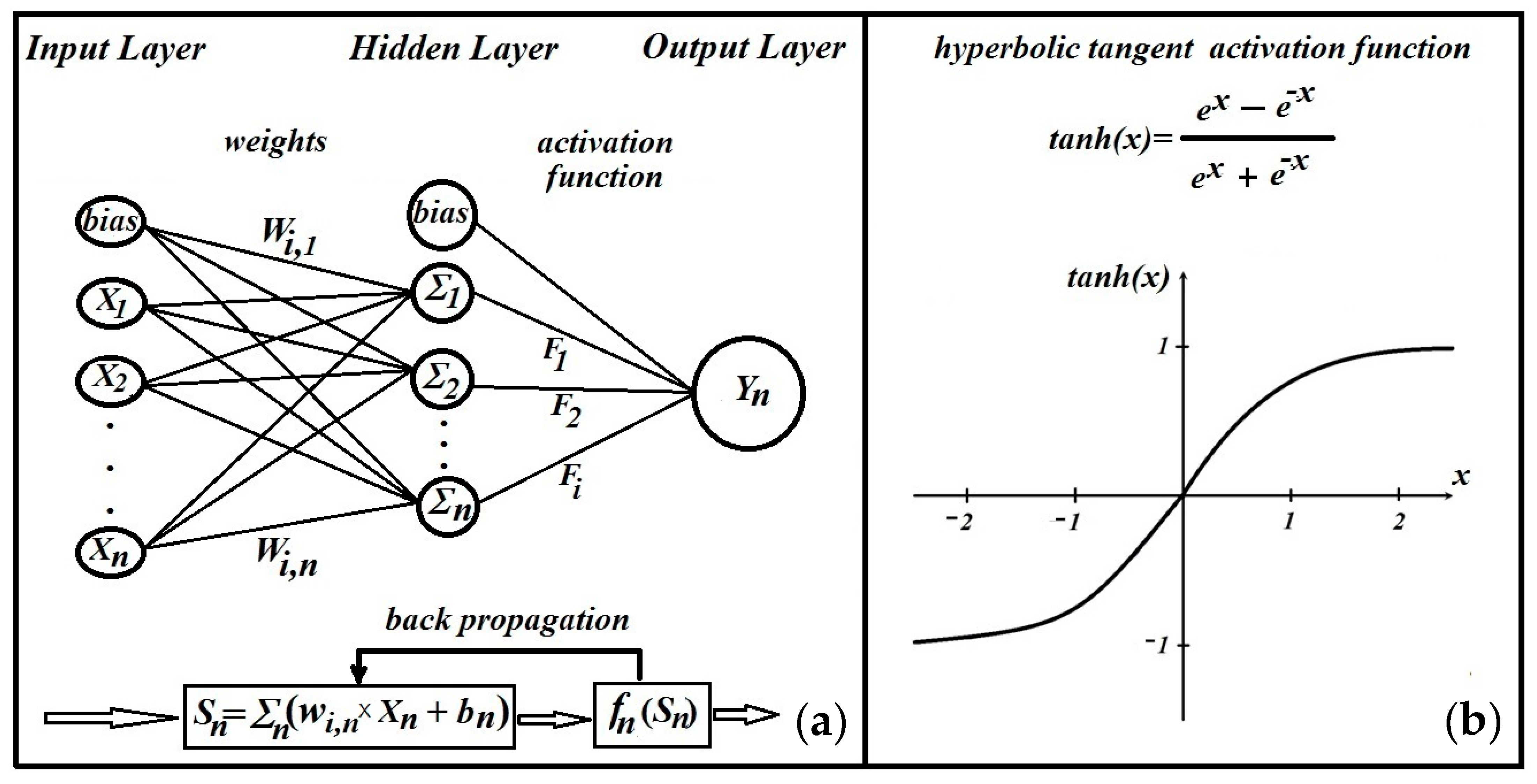
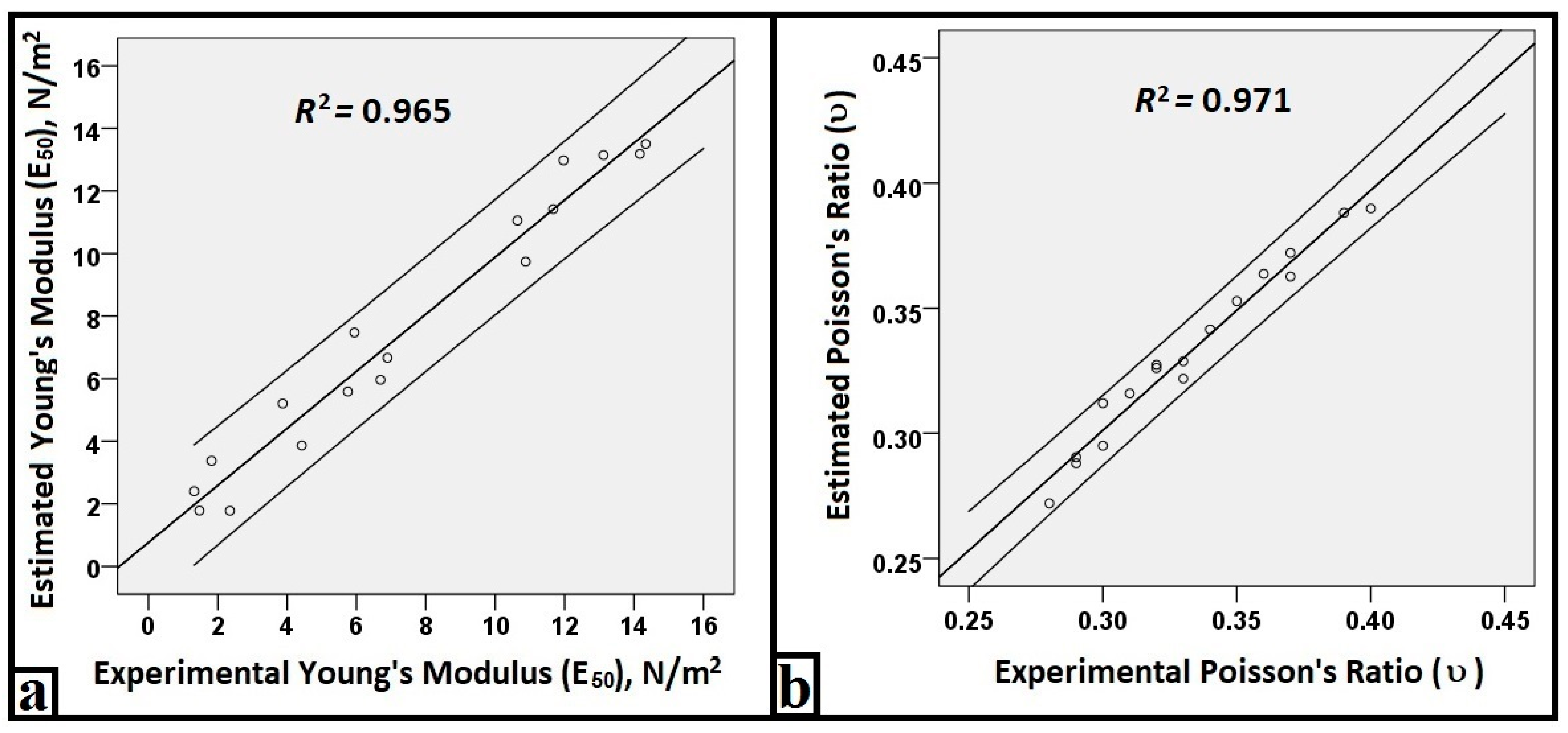
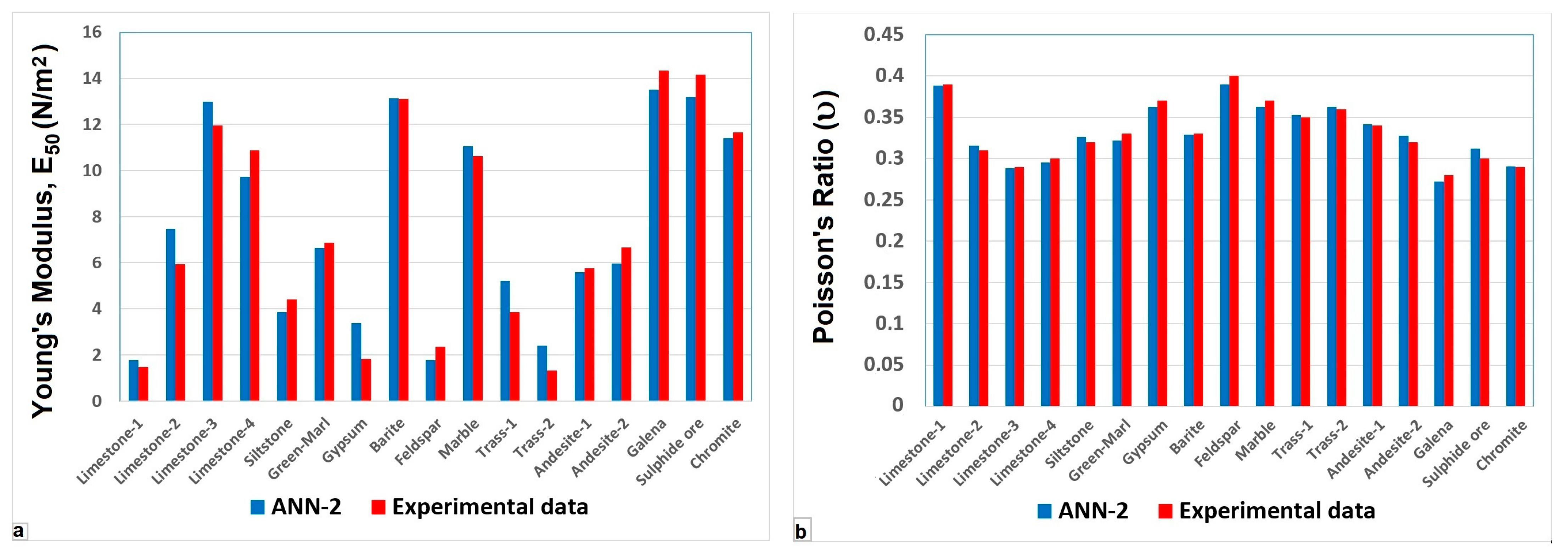
The relationships between the independent variables and the dependent variables can be investigated by using the MLR or MNLR analyses. In estimating the value, the MLR models are expressed linearly and the MNLR models are expressed as a non-linear function. The choice between the MLR and MNLR models is determined by the high determination coefficient of the relationships to be obtained as seen in Equation (2) [8,42].

Y = β₀ + β_1×1 + β₂X₂ + β₃X₃ + β₄X₄ + … + β_nX_n,

(2)

MNLR analysis estimates the model by forming a random non-linear relationship between one or more independent variables and a dependent variable. The typical form of the non-linear relationship is considered as seen in Equation (3).

Y = β₀(X₁^β1)(X₂^β2)(X₃^β3)(X₄^β4) … (X_n^βn),

(3)

where, while Y is the dependent variable, X₁, X₂, X₃, X₄, …, X_n are independent variables. While β₀ is the constant value, β₁, β₂, β₃, β₄, …, β_n are the regression coefficients of linear or non-linear independent variables [42,43,44].

The MLR and MNLR analyses are carried out using a computer software package program since they involve quite complex calculations. In this study, the IBM SPSS 22 statistical software package was used to generate the MLRs between five independent variables (V_p, V_s, V_p/V_s, ρ_d, and SH) and a dependent variable as the output (E₅₀ or υ). The stepwise method in the SPSS program, commonly used in this type of modeling, is a technique for constructing a model by adding or subtracting estimative parameters through a series of F-tests or t-tests. The E₅₀ and υ values of the rock types were introduced as dependent variables (outputs) and X₁ (V_p, m/s), X₂ (V_s, m/s), X₃ (V_p/V_s), X₄ (ρ_d), and X₅ (SH), as independent variables (inputs). However, the p-value and tolerance of V_p/V_s and SH were calculated as near to 0 before the MLR was processed. This indicates that the V_p/V_s and SH variances have the highest probability of multicollinearity when all the variables are taken into account, therefore, V_p/V_s and SH were eliminated from the model. As a result, Equations (4) and (5) are the most reliable regression equations for determining the values of E₅₀ and υ using MLR analysis. Additionally, in Figure 3, the predicted values of E_s and υ are plotted against the experimental values to analyze the accuracy of the MLR model.

E₅₀ = −22.613 − 0.001 × (V_p) + 14.576 × (ρ_d),        R² = 0.582,

(4)

υ = 0.575 − 4.066 × 10⁻⁵ × (V_s) − 0.055 × (ρ_d),        R² = 0.486,

(5)

As the independent variables are evaluated in terms of autocorrelation and multicollinearity, as seen in Equations (4) and (5), three potential independent variables (V_s, V_p/V_s, and SH) were neglected for E₅₀, while two independent variables (V_s and ρ_d) could be evaluated for υ.

Some non-linear regression equations can be converted to a linear equation with an appropriate transformation of the model equation. If the logarithm to base e of Equation (3) was taken, it becomes a linear relationship as seen in Equation (6) [44].

Ln(Y) = Ln(β₀) + β₁Ln(X₁) + β₂Ln(X₂) + β₃Ln(X₃) + β₄Ln(X₄) + β₅Ln(X₅) … β_nLn(X_n),

(6)

and so, an Ln(Y) regression over Ln(X₁), Ln(X₂), Ln(X₃), Ln(X₄), and Ln(X₅) is used to estimate the parameters β₀, β₁, β₂, β₃, β₄, β₅ and β_n [44].

The β₀, β₁, β₂, β₃, β₄, β₅, and β_n coefficients were determined using the stepwise method in the SPSS 22 software program. The stepwise method commonly used in this type of modeling is a technique for constructing a model by adding or subtracting estimative parameters through a series of F-tests or t-tests. The model expressions were coded into the solver based on the fitting result of the linear regression solver and a series of iterations were run. Iteration runs were stopped when the relative reduction between sums of squares was minimized.

In this study, regression relationships between five independent variables and one dependent variable (E₅₀ or υ) were revealed. In both regression relationship equations, the dependent variables X₁, X₂, X₃, X₄, and X₅ are V_p, V_s, V_p/V_s, ρ_d, and SH, respectively. The β_i coefficients were estimated from the experimental results using the SPSS program that applies the least-square method. The R², VIF, T, and p-values were taken into account to evaluate the estimative performance of the regression equations. Then, the best independent variables that did not show autocorrelation and multicollinearity were selected. As a result, the following equations were obtained by MNLR analysis using the best independent variables.

When the independent variables are evaluated in terms of autocorrelation and multicollinearity, as seen in Equations (7) and (8), three potential independent variables (V_s, V_p/V_s, and SH) were neglected for E₅₀, while three independent variables (V_p, V_s, and ρ_d) could be evaluated for υ. Additionally, in Figure 4, the predicted values of E_s and υ are plotted against the experimental values to analyze the accuracy of the NMLR model.

Ln(E₅₀) = 11.519 × (V_p)^−0.716 × (ρ_d)^−5.868,        R² = 0.591,

(7)

Ln(υ) = 0.6555 × (V_p)^0.768 × (V_s)^−0.843 × (ρ_d)^−0.713,        R² = 0.630,

(8)

As a result of the regression analyses, the E₅₀ and υ values were estimated using Equations (4) and (5) by MLR analysis and Equations (7) and (8) by MNLR analysis, and these equations were determined with low coefficients of determination (R²). In addition, since it is not expressed with two independent variables (V_p/V_s and SH), it is not suitable to be considered as a reliable model for the E₅₀ and υ estimation. Therefore, as a solution to such problems, soft computational methods such as ANN can be used.

4.2. ANN Analysis

Using an ANN, a neural network model can be created that can estimate the desired output from one or more inputs. Although various ANN types are used in the literature, the most widely used is the backpropagation ANN (BP-MLP-ANN) [19,36,45,46,47]. The general system structure of a backpropagation MLP-ANN model is shown in Figure 5a, and the hyperbolic tangent activation function is shown in Figure 5b.

In this study, a multilayer perceptron network with hidden layers and an MLP-ANN with a backpropagation architecture were also developed using the neural network function in the SPSS 22.0 program. An ANN model usually has three layers: input layers, hidden layers, and output layers. The input layer was created from five source points such as V_p, V_s, V_p/V_s, ρ_d, and SH. The hidden layer was a non-linear processing unit and can have more than one layer. The output layer was further evaluated by the network and produced the E₅₀ or υ, which are the desired result points from the model. The most applied transfer functions in the literature are the sigmoid and hyperbolic tangent activation functions. The hyperbolic tangent activation function was preferred in this study because it provided the most effective approach. On the other hand, no activation function was used in the output layer. Additionally, 75% of the data was used for training and 25% was used for the testing stage. Five combinations of the variables (V_p, V_s, V_p/V_s, ρ_d, and SH) were investigated using SPSS to determine the optimal network architecture. The best input combinations for the ANN models are given in

Table 3. Details of the four ANN models according to the best input combinations.

Model	Input Combination	Output	R2	RMSE	MAE
ANN-1	Vp, Vs, Vp/Vs, ρd, SH	E50 (N/m2) υ	0.891 0.961	1.490 0.007	0.947 0.005
ANN-2	Vp, Vs, Vp/Vs, SH	E50 (N/m2) υ	0.965 0.971	0.883 0.006	0.699 0.004
ANN-3	Vp, Vs, ρd, SH	E50 (N/m2) υ	0.925 0.956	1.252 0.008	1.037 0.006
ANN-4	Vp, Vs, Vp/Vs, ρd	E50 (N/m2) υ	0.896 0.953	1.478 0.008	1.106 1.106

. These models were selected based on the highest determination coefficient (R²), the lowest root mean square error (RMSE), and the lowest mean absolute error (MAE) to estimate the E_s and υ values of rock materials.

In this study, the hyperbolic tangent function shown in Equation (9) with the output range of [−1, 1] was used. Further, the R², MAE, and RMSE equations shown in Equations (10)–(12) were used to verify the validity of the selected models.

$$\tanh \left(x\right)={\displaystyle \frac{e^x-e^{-x}}{e^x+e^{-x}}}$$

(9)

$$R^2=1-{\displaystyle \frac{\sum {\left(y_i-\widehat{y_{\dot{i}}}\right)}^2}{\sum {\left(y_i-\overline{y}\right)}^2}}$$

(10)

$$MAE={\displaystyle \frac{{\sum }_{i=1}^n\left|y_i-\widehat{y_{\dot{i}}}\right|}{n}}$$

(11)

$$RMSE=\sqrt{{\displaystyle \frac{{\sum }_{i=1}^n{\left(y_i-\widehat{y_{\dot{i}}}\right)}^2}{n}}}$$

(12)

where n, y_i, ў, and ŷ_i are the number of experiments, the experimental values, the mean of the experimental values, and the estimated values, respectively.

The R², RMSE, and MAE values calculated to determine the validity of the ANN models are presented in Table 3. When Table 3 is examined, R² values higher than 0.80 mean that there are relationships with acceptable accuracy for these four models. However, when the R², RMSE, and MAE values in Table 3 were examined, it was determined that ANN-2 gave more accurate estimates than the other models. The R² values of 0.965 and 0.971 obtained by the ANN-2 model for E₅₀ and υ, respectively, indicate that the models have a very good relationship. The estimated error values for the E₅₀ and υ were 0.883 and 0.006 for the RMSE and 0.699 and 0.004 for the MAE, respectively. The ANN-3 was ranked as the second best model. The results of the ANN-1 and ANN-4 models were also acceptable for estimating the E₅₀ and υ. When the normalized importance values were examined, the Shore hardness (SH) was found to have a great effect of 100% on both the E₅₀ and υ values.

Figure 6 shows the best model architecture (ANN-2), which is shown to consist of one input layer of four variables, one hidden layer of 10 neurons, and one output layer of one variable (a 4-10-1 structure) by using the activation functions. Additionally, in Figure 7 the predicted values of E_s and υ are plotted against the experimental values to analyze the accuracy of the ANN-2 model.

4.3. Comparison of Models

The E₅₀ and υ parameters of rock materials were compared in terms of the estimated values using the MLR, MNLR, and ANN models. As a result, it was revealed that the MLR and MNLR models could not estimate either E₅₀ or υ parameters very well. Additionally, because of the complexity of the fracture process in rock materials, it is an expected result that the coefficients of determinate (R²) of the MLR and MNLR models for E₅₀ and υ are low. On the other hand, the ANN models with the highest R² values for estimating the E₅₀ and υ parameters were found to be much more suitable than the MLR and MNLR models.

A comparison of the estimated values generated by the ANN-2 model for each of the 17 experimental data points of the E₅₀ and υ for the rock type samples is shown in Figure 8. Apparently, the results indicate that the ANN-2 model was able to estimate both the E₅₀ and υ values very well within the acceptance limit. On the other hand, the estimated values of the other ANN models were significantly different in accuracy from all the experimental E₅₀ and υ values. In addition, the ANN-2 model has the lowest RMSE and MAE and the highest R² values (see Table 3), which shows that it will be much more suitable than the other ANN models.

Although it is generally accepted that a substantial amount of data is needed to train the neural network, it is important to note that ore samples such as galena, chromite, and sulfur ore have not been used in any previous study. These specific properties are examined for the first time in the context of rock mechanics.

5. Conclusions

This research aims to aid in the development of estimation models with the highest accuracy for determining the E₅₀ and υ parameters of different rock types using non-destructive measurement methods (V_p, V_s, V_p/V_s, ρ_d, and SH). For this purpose, 17 different rock types were considered, and multiple measurements were made to estimate the E₅₀ and υ with the best possible accuracy.

Model approaches were based on input data (V_p, V_s, V_p/V_s, ρ_d, and SH). These approaches did not yield satisfactory results in the multiple regression analyses (MLR and MNLR) expressed as correlation coefficients (R² = 0.486–0.630). However, ANN models developed using the same experimental data produced results with higher determination coefficients (R² = 0.891–0.971). These results indicate that ANN models are preferable for the estimation and evaluation of E₅₀ and υ compared to regression analysis models. From these results, it was determined that all four ANN models were able to predict both E₅₀ and υ with higher accuracy and minimal errors. Among the ANN architectures tested, ANN-2, with four input variables (V_p, V_s, V_p/V_s, and SH), 10 neurons, and one output variable (E₅₀ or υ), was the best architecture (4-10-1 structure). In addition, the results of sensitivity analysis of both E₅₀ and υ values to input variables showed that Shore hardness (SH) was the most sensitive variable.

This study is the first in the literature to use a highly diverse sample set, including magmatic ores such as chromite, galena, and sulfide ores, in modeling. Overall, such estimation models will be beneficial to more engineers in the sector if different geological types and larger specimen sets are evaluated using similar research methods in the coming years.

References

1. ISRM. Rock Characterization, Testing and Monitoring, ISRM Suggested Methods; International Society for Rock Mechanic: Lisbon, Portugal, 1981; p. 211. [Google Scholar]
2. ASTM. Soil and Rock Building Stones: Annual Book of ASTM Standards; ASTM Publication: Philadelphia, PA, USA, 1984; Volume 4.08. [Google Scholar]
3. Ghafoori, M.; Rastegarnia, A.; Lashkaripour, G.R. Estimation of static parameters based on dynamical and physical properties in limestone rocks. J. Afr. Earth Sci. 2018, 137, 22–31. [Google Scholar] [CrossRef]
4. Van Heerden, W.L. General relations between static and dynamic moduli of rocks. Int. J. Rock Mech. Min. Sci. Geomech. Abstr. 1987, 24, 381–385. [Google Scholar] [CrossRef]
5. Pappalardo, G. Correlation between P-wave velocity and physical-mechanical properties of intensely jointed dolostones, Peloritani mounts, NE Sicily. Rock Mech. Rock Eng. 2015, 48, 1711–1721. [Google Scholar] [CrossRef]
6. Chen, X.; Xu, Z. The ultrasonic P-wave velocity-stress relationship of rocks and its application. Bull. Eng. Geol. Environ. 2016, 76, 661–669. [Google Scholar] [CrossRef]
7. King, M.S. Static and dynamic properties of rocks from the Canadian Shield. Int. J. Rock Mech. Min. Sci. Geomech. Abstr. 1983, 20, 237–245. [Google Scholar] [CrossRef]
8. Armaghani, D.J.; Mohamad, E.T.; Momeni, E.; Monjezi, M.; Narayanasamy, M.S. Prediction of the strength and elasticity modulus of granite through an expert artificial neural network. Arab. J. Geosci. 2016, 9, 48. [Google Scholar] [CrossRef]
9. Teymen, A. Statistical models for estimating the uniaxial compressive strength and elastic modulus of rocks from different hardness test methods. Heliyon 2021, 7, e06891. [Google Scholar] [CrossRef]
10. Khandelwal, M. Correlating P-wave velocity with the physic-mechanical properties of different rocks. Pure Appl. Geophys. 2013, 170, 507–514. [Google Scholar] [CrossRef]
11. Raj, K.; Pedram, R. Correlations between direct and indirect strength test methods. Int. J. Min. Sci. Technol. 2015, 25, 355–360. [Google Scholar]
12. Sachpazis, C.I. Correlating Schmidt hardness with compressive strength and Young’s modulus of carbonate rocks. Bull. Int. Assoc. Eng. Geol. 1990, 42, 75–83. [Google Scholar] [CrossRef]
13. Yilmaz, I.; Sendir, H. Correlation of Schmidt hardness with unconfined compressive strength and Young’s modulus in gypsum from Sivas (Turkey). Eng. Geol. 2002, 66, 211–219. [Google Scholar] [CrossRef]
14. Hoek, E.; Diederichs, M.S. Empirical estimation of rock mass modulus. Int. J. Rock Mech. Min. Sci. 2006, 43, 203–215. [Google Scholar] [CrossRef]
15. Isik, N.S.; Ulusay, R.; Doyuran, V. Deformation modulus of heavily jointed–sheared and blocky greywackes by pressure meter tests: Numerical, experimental and empirical assessments. Eng. Geol. 2008, 101, 269–282. [Google Scholar] [CrossRef]
16. Palchik, V. On the ratios between elastic modulus and uniaxial compressive strength of heterogeneous carbonate rocks. Rock Mech. Rock Eng. 2011, 44, 121–128. [Google Scholar] [CrossRef]
17. Alemdag, S.; Gurocak, Z.; Gokceoglu, C. A simple regression based approach to estimate deformation modulus of rock masses. J. Afr. Earth Sci. 2015, 110, 75–80. [Google Scholar] [CrossRef]
18. Feng, X.; Jimenez, R. Estimation of deformation modulus of rock masses based on Bayesian model selection and Bayesian updating approach. Eng. Geol. 2015, 199, 19–27. [Google Scholar] [CrossRef]
19. Sonmez, H.; Gokceoglu, C.; Nefeslioglu, H.A.; Kayabasi, A. Estimation of rock modulus: For intact rocks with an artificial neural network and for rock masses with a new empirical equation. Int. J. Rock Mech. Min. Sci. 2006, 43, 224–235. [Google Scholar] [CrossRef]
20. Yasar, E.; Erdogan, Y. Estimation of rock physicomechanical properties using hardness methods. Eng. Geol. 2004, 71, 281–288. [Google Scholar] [CrossRef]
21. Shalabi, F.I.; Cording, E.J.; Al-Hattamleh, O.H. Estimation of rock engineering properties using hardness tests. Eng. Geol. 2007, 90, 138–147. [Google Scholar] [CrossRef]
22. Karakus, M.; Kumral, M.; Kilic, O. Predicting elastic properties of intact rocks from index tests using multiple regression modeling. Int. J. Rock Mech. Min. Sci. 2005, 42, 323–330. [Google Scholar] [CrossRef]
23. Kahraman, S.; Yeken, T. Determination of physical properties of carbonate rocks from P-wave velocity. Bull. Eng. Geol. Environ. 2008, 67, 277–281. [Google Scholar] [CrossRef]
24. Sharma, P.K.; Singh, T.N. A correlation between P-wave velocity, impact strength index, slake durability index and uniaxial compressive strength. Bull. Eng. Geol. Environ. 2008, 67, 17–22. [Google Scholar] [CrossRef]
25. Yagiz, S. P-wave velocity test for assessment of geotechnical properties of some rock materials. Bull. Mater. Sci. 2011, 34, 947–953. [Google Scholar] [CrossRef]
26. Concu, G.D.; Nicolo, B.; Valdes, M. Prediction of building limestone physical and mechanical properties by means of ultrasonic P-wave velocity. Sci. World J. 2014, 2014, 508073. [Google Scholar] [CrossRef] [PubMed]
27. Korkanc, M.; Solak, B. Estimation of engineering properties of selected tuffs by using grain/matrix ratio. J. Afr. Earth Sci. 2016, 120, 160–172. [Google Scholar] [CrossRef]
28. Stan-Kłeczek, I. The study of the elastic properties of carbonate rocks on a base of laboratory and field measurement. Acta Montan. Slovaca 2016, 21, 76–83. [Google Scholar]
29. Huang, Y.; Wänstedt, S. The introduction of neural network system and its applications in rock engineering. Eng. Geol. 1998, 49, 253–260. [Google Scholar] [CrossRef]
30. Meulenkamp, F.; Alvarez-Grima, M. Application of neural networks for the prediction of the unconfined compressive strength (UCS) from Equotip hardness. Int. J. Rock Mech. Min. Sci. 1999, 36, 29–39. [Google Scholar] [CrossRef]
31. Baykasoglu, A.; Gullu, H.; Canakcı, H.; Ozbakır, L. Prediction of compressive and tensile strength of limestone via genetic programming. Expert Syst. Appl. 2008, 35, 111–123. [Google Scholar] [CrossRef]
32. Zorlu, K.; Gokceoglu, C.; Ocakoglu, F.; Nefeslioglu, H.A.; Acikalin, S. Prediction of uniaxial compressive strength of sandstones using petrography-based models. Eng. Geol. 2008, 96, 141–158. [Google Scholar] [CrossRef]
33. Dehghan, S.; Sattari, G.H.; Chehreh, C.S.; Aliabadi, M.A. Prediction of unconfined compressive strength and modulus of elasticity for travertine samples using regression and artificial neural. New Min. Sci. Technol. 2010, 20, 41–46. [Google Scholar]
34. Jang, H.; Topal, E. Optimizing over break prediction based on geological parameters comparing multiple regression analysis and artificial neural network. Tunn. Undergr. Space Technol. 2013, 38, 161–169. [Google Scholar] [CrossRef]
35. Momeni, E.; Armaghani, D.J.; Hajihassani, M.; Amin, M.F.M. Prediction of uniaxial compressive strength of rock samples using hybrid particle swarm optimization-based artificial neural networks. Measurement 2015, 60, 50–63. [Google Scholar] [CrossRef]
36. Mottahedi, A.; Sereshki, F.; Ataei, M. Development of overbreak prediction models in drill and blast tunneling using soft computing methods. Eng. Comput. 2018, 34, 45–58. [Google Scholar] [CrossRef]
37. ASTM D7012-14e1; Standard Test Methods for Compressive Strength and Elastic Moduli of Intact Rock Core Specimens under Varying States of Stress and Temperatures. American Society for Testing and Materials International: West Conshohocken, PA, USA, 2017.
38. ASTM D2845-08; Standard Test Method for Laboratory Determination of Pulse Velocities and Ultrasonic Elastic Constants of Rock (Withdrawn 2017). American Society for Testing and Materials International: West Conshohocken, PA, USA, 2008. [CrossRef]
39. Telford, W.M.; Geldart, L.P.; Sheriff, R.E.; Keys, D.A. Applied Geophysics; Cambridge University Press: Cambridge, UK, 1976. [Google Scholar]
40. Tumac, D.; Bilgin, N.; Feridunoglu, C.; Ergin, H. Estimation of rock cuttability from Shore hardness and compressive strength properties. Rock Mech. Rock Eng. 2007, 40, 477–490. [Google Scholar] [CrossRef]
41. ISRM. Suggested methods for determining hardness and abrasiveness of rocks, Part 3. In Rock Characterization, Testing and Monitoring; ISRM Suggested Methods; Brown, E.T., Ed.; Pergamon: Oxford, UK, 1981; pp. 101–103. [Google Scholar]
42. Kutner, M.H.; Nachtsheim, C.J.; Neter, J.; Li, W. Applied Linear Statistical Models, 5th ed.; McGraw-Hill Higher Education: New York, NY, USA, 2004. [Google Scholar]
43. Paulson, D.S. Handbook of Regression and Modelling; Chapman & Hall/CRC: Taylor & Francis Group: Boca Raton, FL, USA, 2007. [Google Scholar]
44. Bilgili, M.; Ozgoren, M. Daily total global solar radiation modeling from several meteorological data. Meteorol. Atmos. Phys. 2011, 112, 125–138. [Google Scholar] [CrossRef]
45. Hair, J.F.J.; Anderson, R.E.; Tatham, R.L.; Black, W.C. Multivariate Data Analysis, 5th ed.; Prentice Hall PTR: New York, NY, USA, 1998. [Google Scholar]
46. Jain, A.K.; Mao, J.; Mohiddin, K.M. Artificial neural networks: A tutorial. Comp. IEEE 1996, 29, 31–44. [Google Scholar] [CrossRef]
47. Schalkoff, R.J. Artificial Neural Network; McGraw-Hill: New York, NY, USA, 1997. [Google Scholar]
Figure 1. The core specimens taken from the rock blocks such as gypsum (a), marble (b), trass (c), galena (d); electrical resistance lateral and axial strain gauges glued to the feldspar core specimen (e); strain-gauge bonded rock specimen under compression (f); Shore Scleroscope C-2 used in the experiments (g).
Mining 04 00036 g001
Figure 2. Specimen types used for sonic wave velocity measurement (a); working principle of the sonic viewer instrument used in the experiments (b).
Mining 04 00036 g002
Figure 3. Comparison of the MLR estimated values and the experimental values for the E50 (a) and υ (b) of the rock materials.
Mining 04 00036 g003
Figure 4. Comparison of the NMLR estimated values and the experimental values for the E50 (a) and υ (b) of the rock materials.
Mining 04 00036 g004
Figure 5. The architecture of an ANN model structure (a) and the hyperbolic tangent activation function (b).
Mining 04 00036 g005
Figure 6. The architecture of the ANN-2 model used to estimate the E50 (a) and υ (b) of the rock materials.
Mining 04 00036 g006
Figure 7. Comparison of the ANN-2 estimated values and the experimental values for the E50 (a) and υ (b) of the rock materials.
Mining 04 00036 g007
Figure 8. Comparison plots of the estimated values generated by the ANN-2 model vs. the experimental values of E50 (a) and υ (b) for the rock materials.
Mining 04 00036 g008