
On the Dilatancy of Fine-Grained Soils

Abstract
:1. Notation and Symbols
2. Introduction
- (i)
- at the beginning, , and the rate-dependent behaviour of a plastic clay achieves its maximum.
- (ii)
- After some cycles of constant stress amplitude, the mean effective pressure decreases while the void ratio and the preconsolidation pressure remain constant, i.e., the current OCR increases.
- (iii)
- For , the rate dependency of the clay decays sparsely and, depending on the subjected loading magnitude, the response of the material is contractant. This leads to a reduction in the effective mean stress p, resulting in a decay of the shear strength and of the barotropic stiffness.
- (iv)
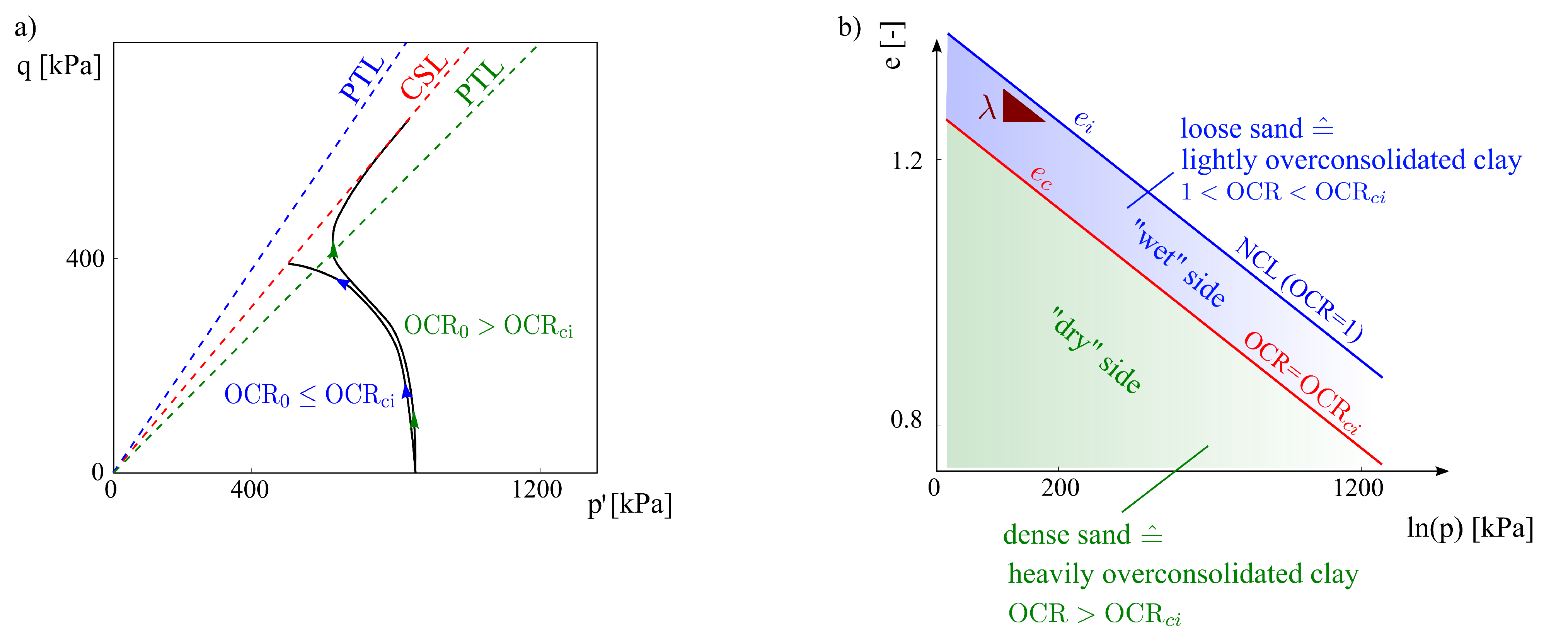
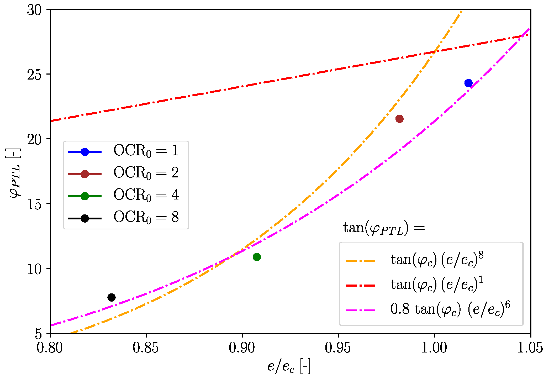
- Towards higher , a significant reduction in the viscous effects is evident. We will show that, in this case, the phase transformation line (PTL) lies below the critical state line. Thus, besides contractancy, dilatant behaviour can also be observed when overpassing the PTL (similar to the behaviour of sands, widely reported in the literature [11,14,19,20]).
3. Dilatancy of Fine-Grained Soils Evaluated from Monotonic and Cyclic Triaxial Tests
3.1. Basic Postulates and Assumptions
3.2. Overconsolidation Ratio
3.3. Results for Kaolin
3.3.1. Triaxial Tests under Monotonic Loading
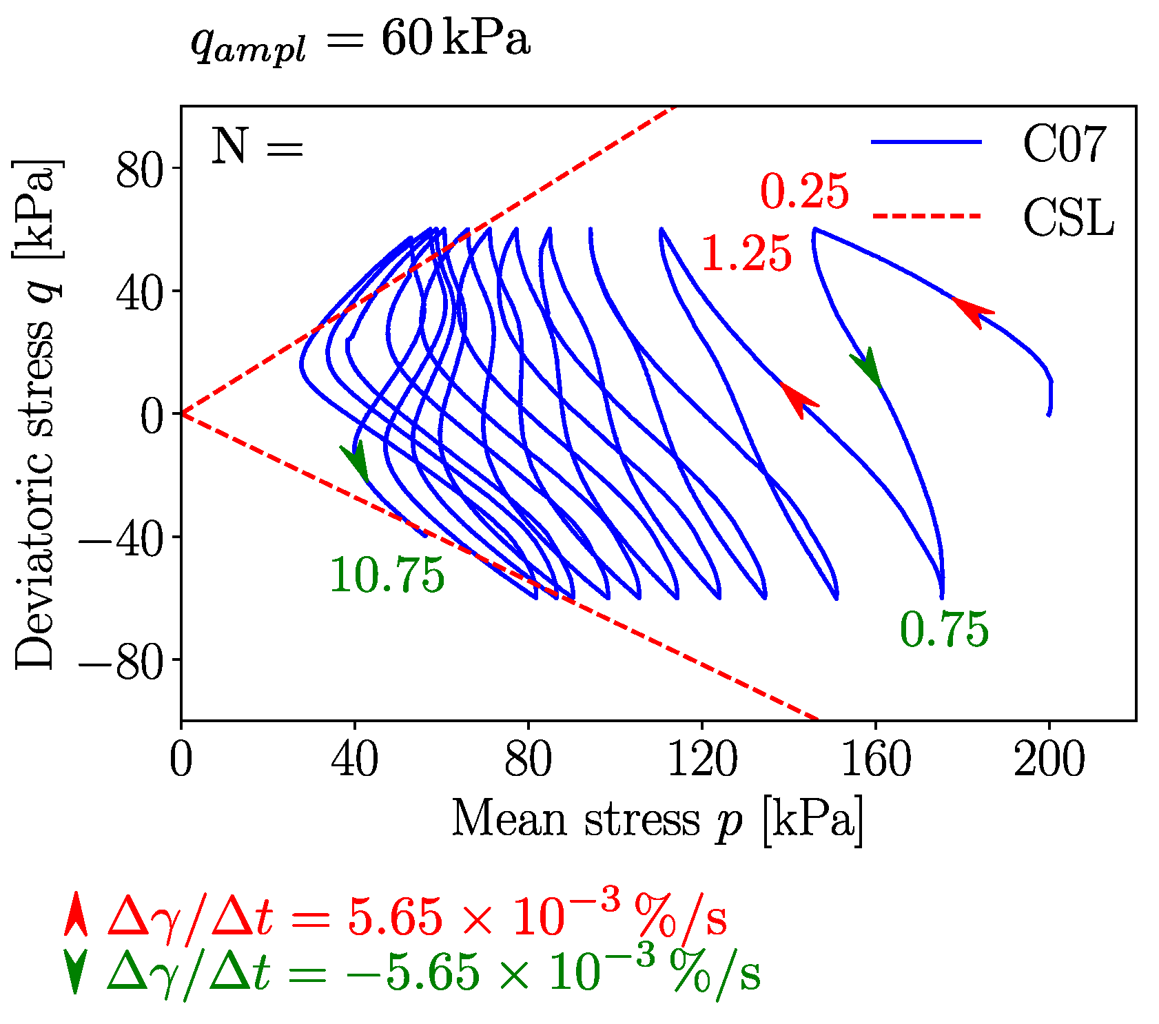
3.3.2. Triaxial Tests under Cyclic Loading
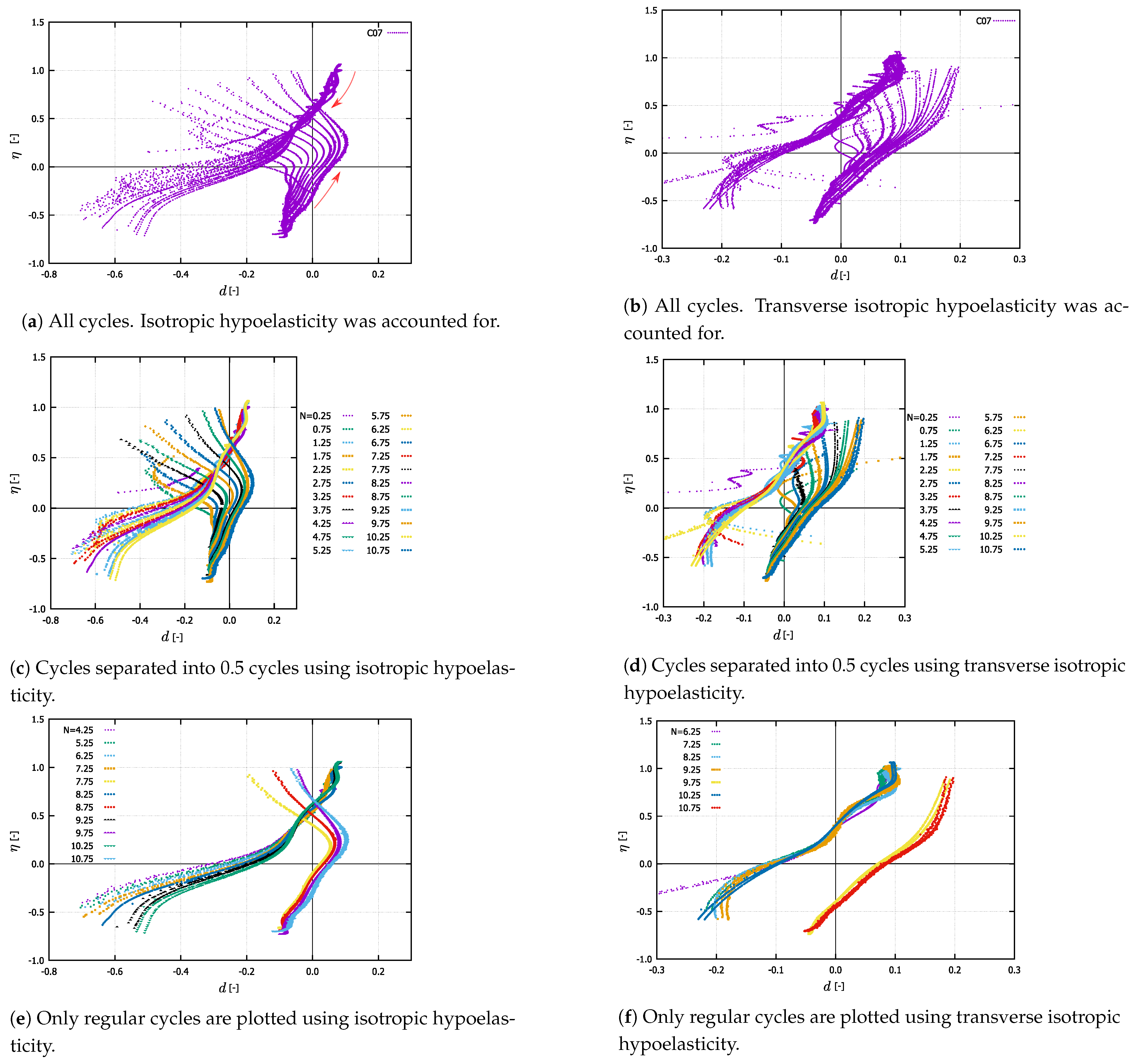
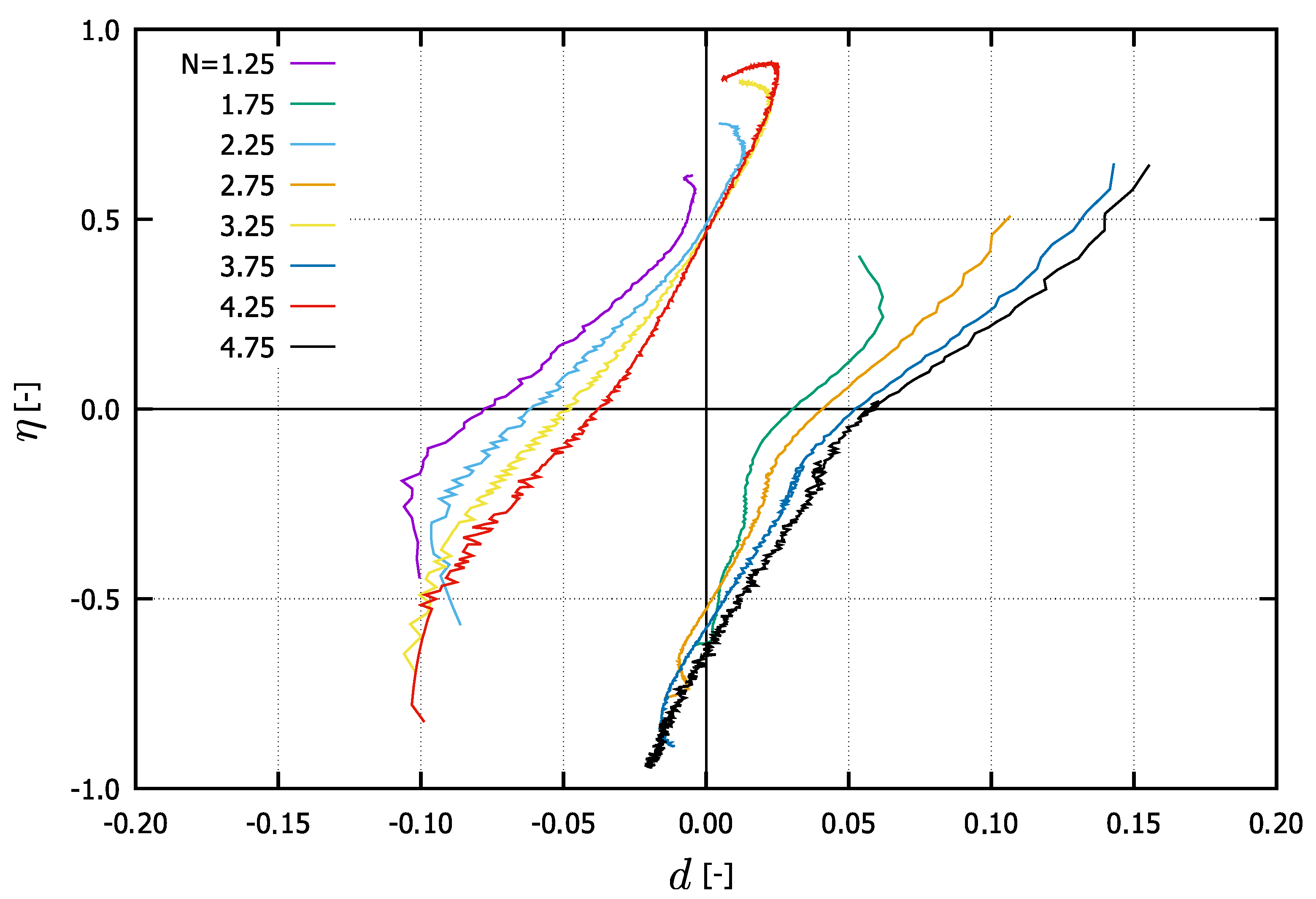
- In Figure 7a–d, all cycles are considered. A comparison between the figures on the left and those on the right (hence between the approaches proposed in Section 3.1) shows that the main difference is noticed at loading reversals in triaxial extension. These discrepancies are particularly noticeable when comparing Figure 7a with Figure 7d or Figure 7c with Figure 7d. Thereby, the evaluation accounting for isotropic hypoelasticity leads to dilatancy at the stress reversal points (from loading in triaxial compression to loading in triaxial extension). On the other hand, the use of transversal isotropic hypoelasticity leads to increased contractancy at stress reversals from loading in triaxial compression to loading in triaxial extension. The latter observations are in accordance with studies conducted on sand, e.g., [4], even though some data scatter can be observed in these figures. At this point, one should be aware that no data points have been omitted during these evaluations.
- On the other hand, only regular (not initial) cycles have been considered in Figure 7e,f. Hereby, the data scatter is almost absent and the aforementioned trends are even more pronounced. Hence, a correct description of the elasticity is essential for the evaluation of the dilatancy curves. Of course, as soon as a hyperelastic potential is evaluated experimentally and described mathematically for Kaolin, it makes sense to validate these evaluations again. At the moment, it may be concluded that the transversal isotropic hypoelasticity corresponds better than the isotropic hypoelasticity to the behaviour of Kaolin.
- This evaluation scheme can furthermore be verified by conducting tests with (e.g., in hollow cylinder apparatus). Thereby, intermediate small loops of unloading–reloading elastic cycles are also necessary to evaluate the portion of and should be the target of further research. Note that, in this work, instead of was used. As claimed in some works [4,9,52], the use of would reduce the scattering in the dilatancy vs. stress ratio relations for sand.
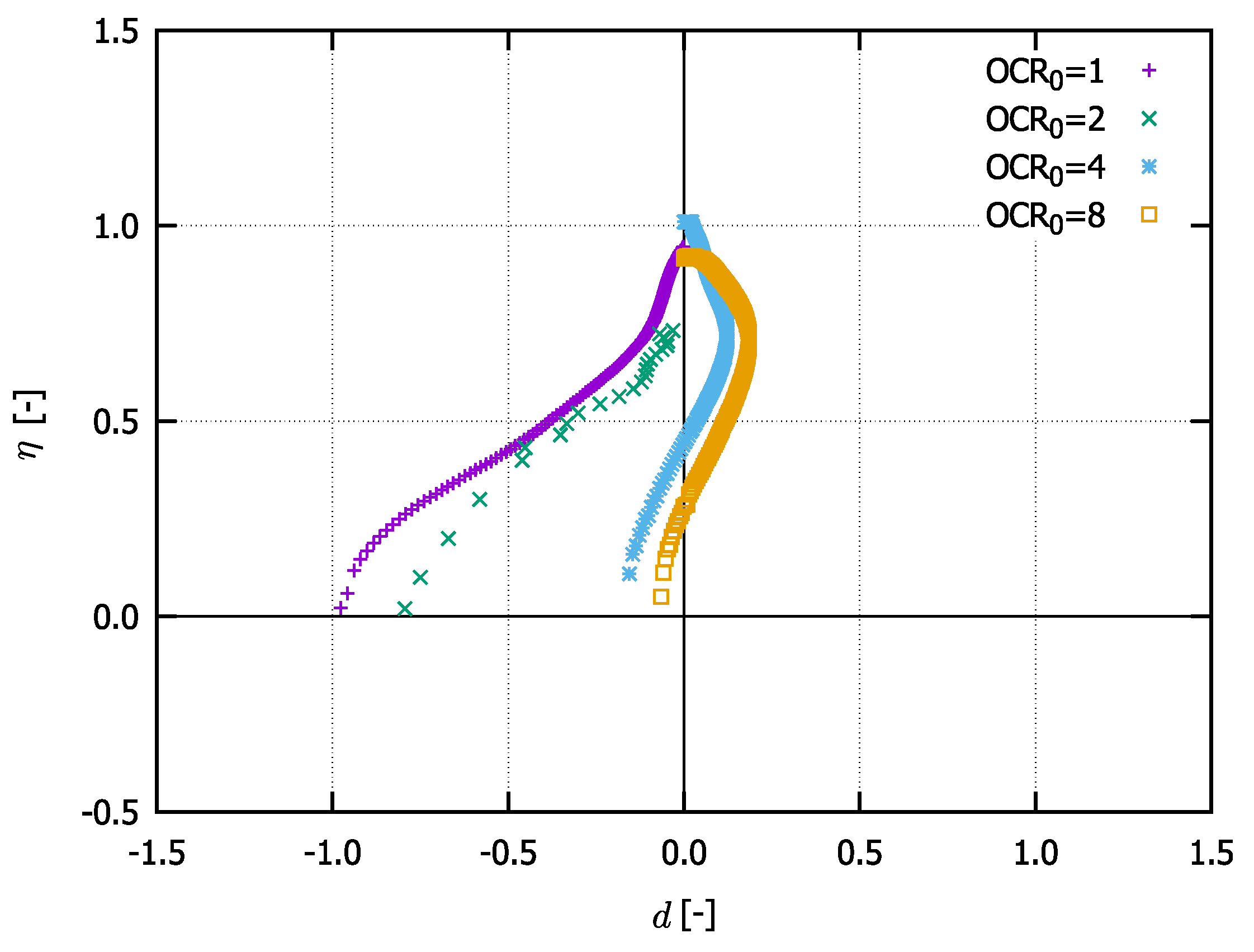
- As stated also in [40], the “elastic dilatancy” after reversals is evident, for example, in Figure 7c. Using the transversal isotropic hypoelasticity, it is eliminated, as depicted in Figure 7d. This elasticity provokes an increase in the effective mean stress, resulting in a slope to the upper left of the effective stress path [17,18,40]. It is well known that clays possess a greater elastic locus compared to sands. If the elasticity was isotropic, then the described path would be vertical with respect to the axis. Thus, we can consider the inherent anisotropy to be responsible for an even lower reduction in effective pressure after loading reversal. For sands, in contrast, after a loading reversal, the largest contractancy has been observed. Hence, the greater elastic regime of fine-grained soils cannot be overcome through the contractancy and it results in a non-vanishing mean effective pressure at cyclic mobility .This effect may be explained by the inherent anisotropy caused by specific sedimentation along a given axis. Thus, the question arises as to whether a cutting direction of the sample may be found at which the soft soil would also liquify (weak axis). This requires further research. Some authors [25,28,36] explain the non-liquefaction behaviour of clays in terms of the viscosity and its cohesive effect. Supposing this to be true, then the intensity of creep would not vanish with a higher overconsolidation ratio, as has been experimentally documented in [21,53]. On the other hand, this implies the existence of a special strain rate (loading velocity) with which the cyclic undrained shearing of a clay sample would result in liquefaction. Following our theory, this would be the case for the greatest velocity ; hence, the viscous effects would not have time to develop. The experiments presented in [17] and the discussions made in [40] hint at this phenomenon. However, further research work is required in order to shed more light and explain this phenomenon.
3.4. Results for Lower Rhine Clay
4. Constitutive Description of the State-Dependent Dilatancy for Cohesive Soils
4.1. Generalisation to Multiaxial Space
4.2. Dilatancy Rule
4.3. Incorporation of Dilatancy into a General Hypoplastic Model
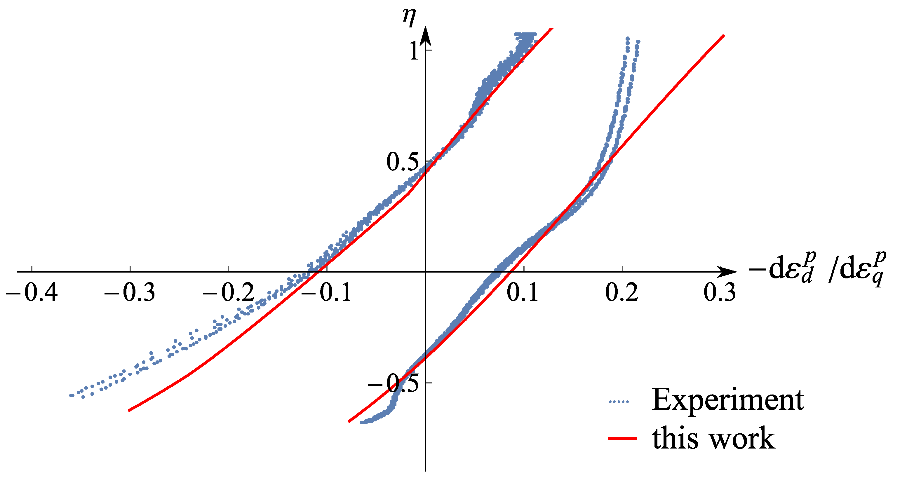
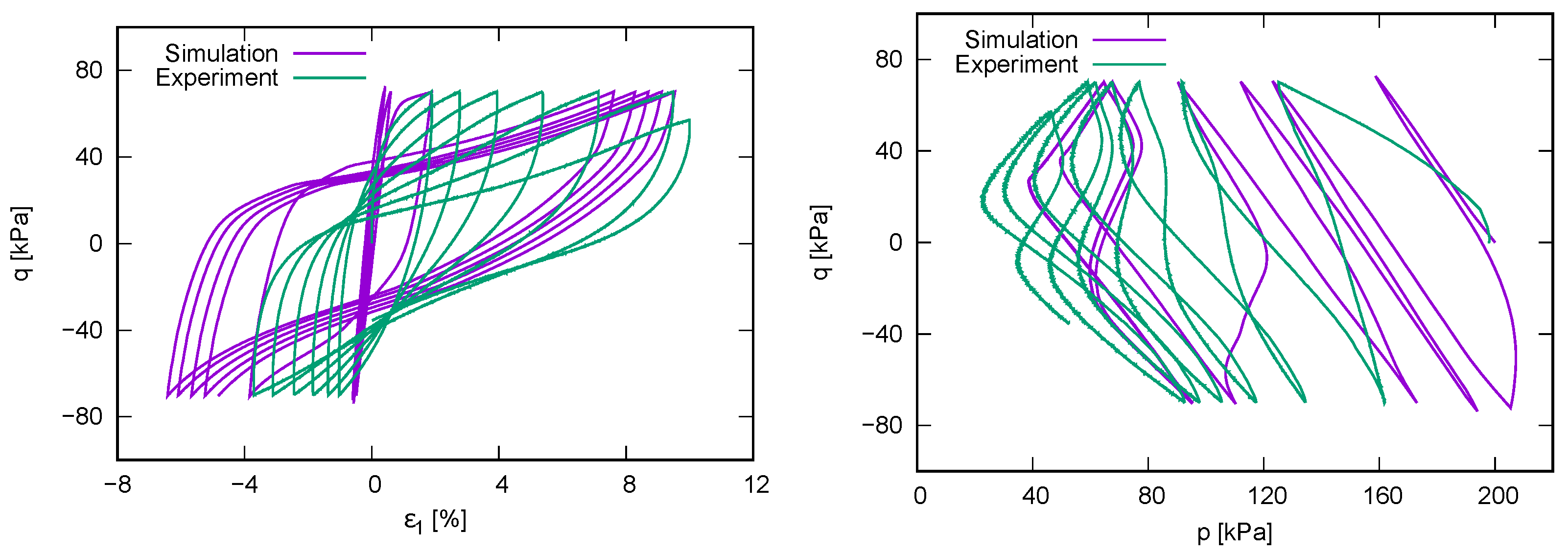
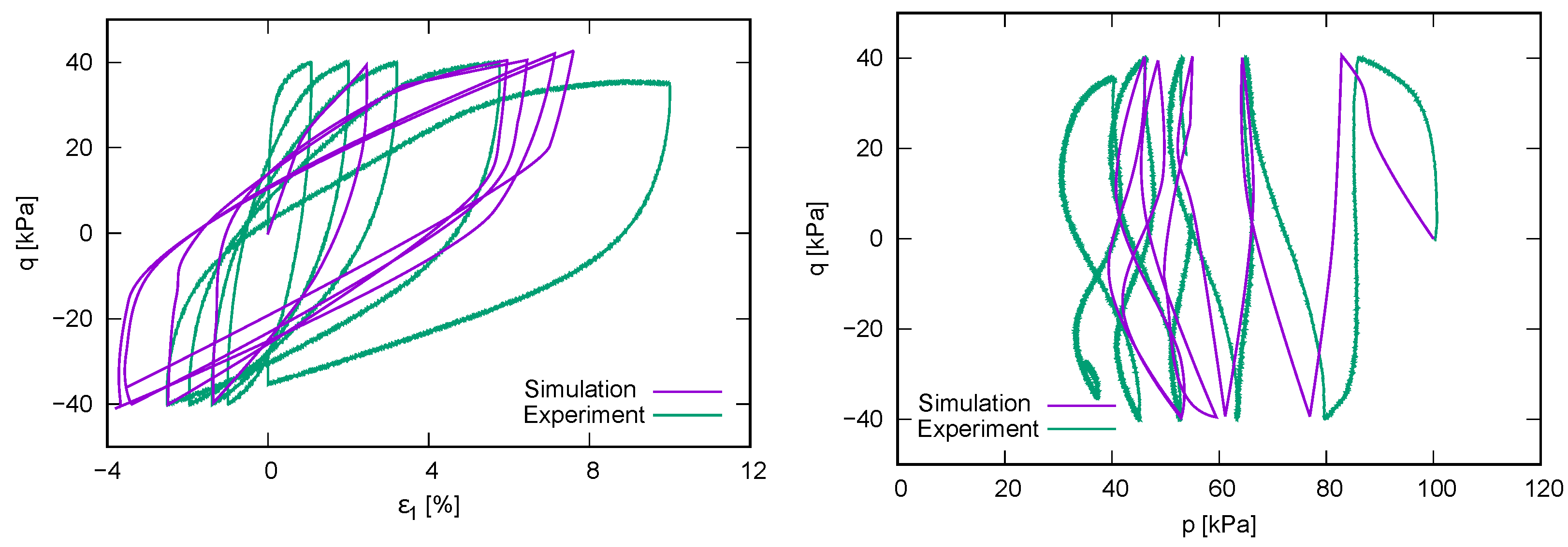
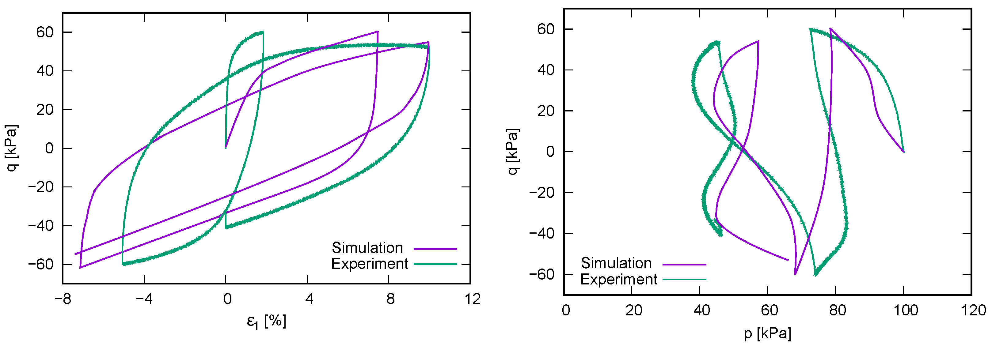
4.4. Simulations with Experiments
5. Conclusions
Author Contributions
Funding
Institutional Review Board Statement
Informed Consent Statement
Data Availability Statement
Acknowledgments
Conflicts of Interest
Nomenclature
| plasticity index | |
| mean effective stress | |
| q | deviatoric (effective) stress |
| isometric effective stress invariants | |
| stress ratio | |
| stress ratio at the critical state | |
| M | slope of the critical state line |
| d | dilatancy |
| stress ratio at the phase transformation line | |
| (initial) overconsolidation ratio | |
| total strain rate | |
| elastic strain rate | |
| plastic strain rate | |
| volumetric strain rate | |
| deviatoric strain | |
| 𝗘 | stiffness tensor |
| components of the stiffness tensor | |
| e | void ratio |
| shear strain increment | |
| time increment | |
| N | number of cycles |
| 𝗤 | rotation tensor |
| normal vector | |
| anisotropic coefficient | |
| auxiliary variables | |
| compression index | |
| swelling index | |
| deviatoric stress amplitude | |
| friction angle | |
| dilatancy angle | |
| flow rule | |
| Y | degree of nonlinearity |
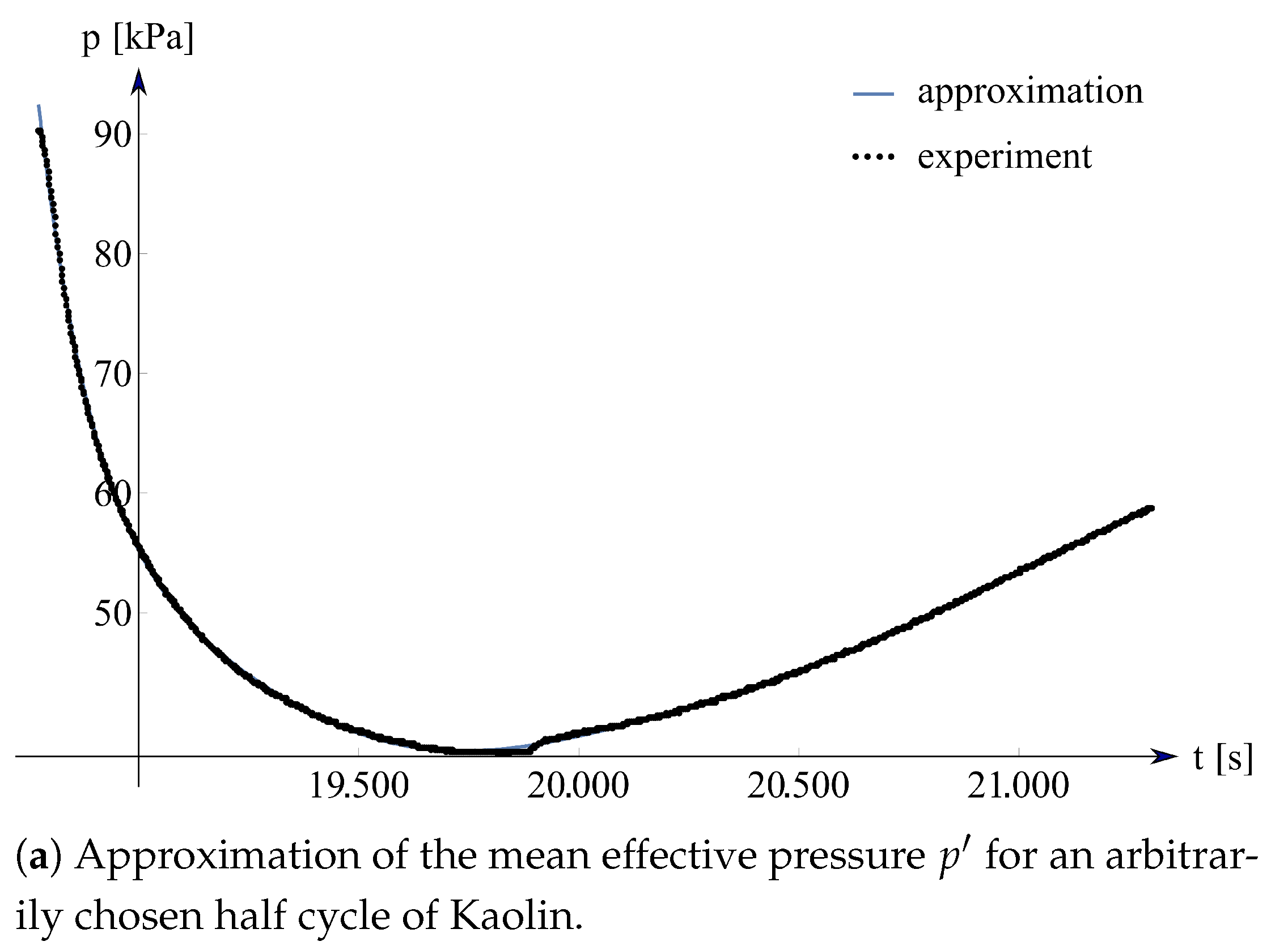
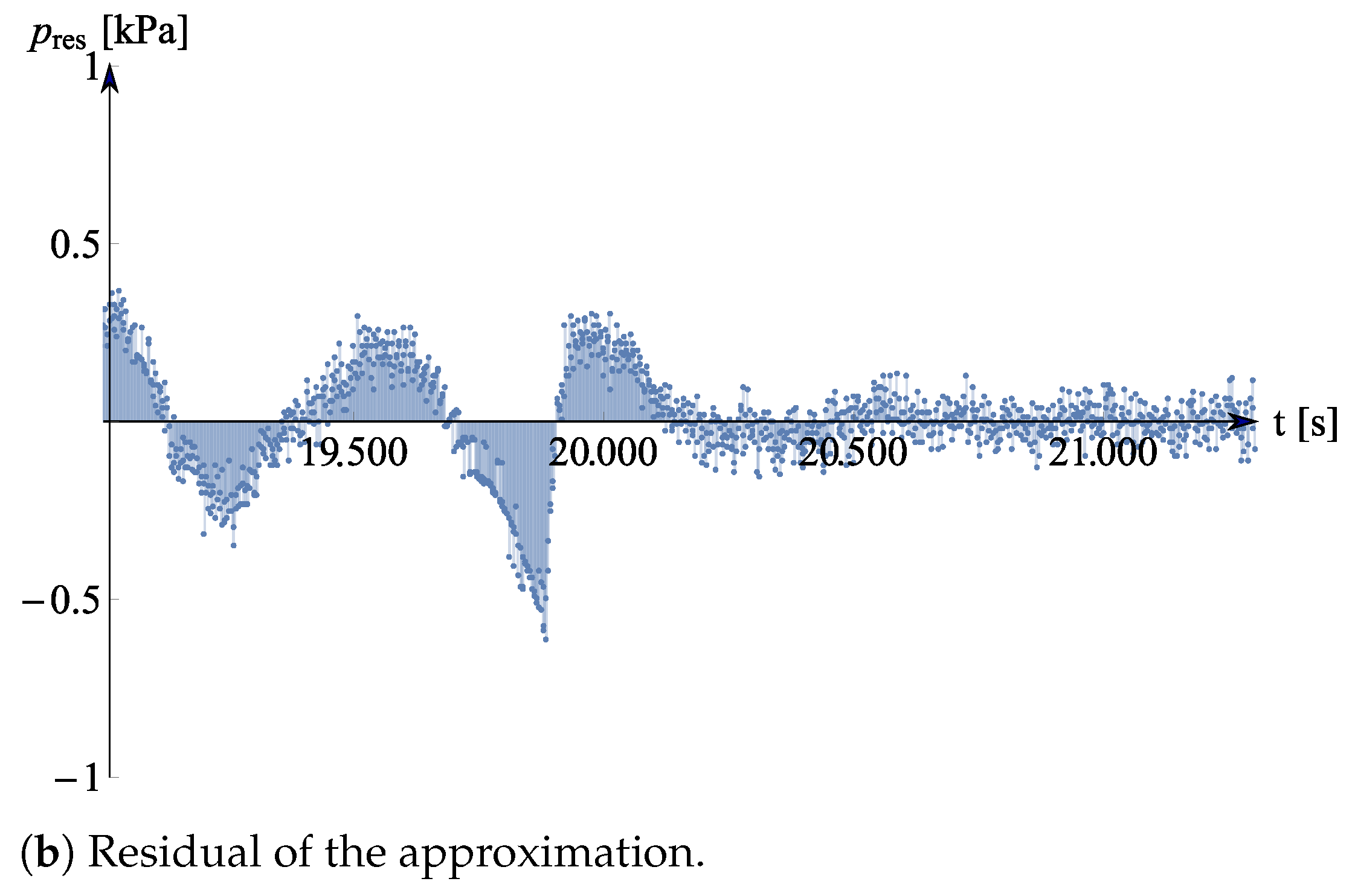
Appendix A. Approximation of the Mean Effective Pressure with Time t
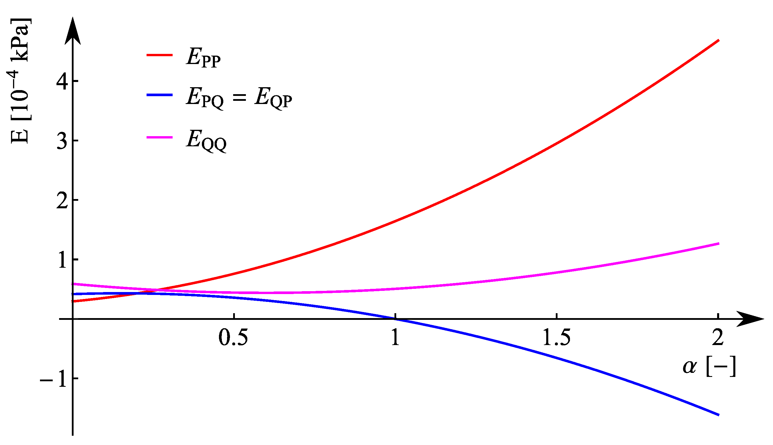
Appendix B. Transversal Isotropic Hypoelasticity
References
- Cattoni, E.; Tamagnini, C. On the seismic response of a propped r.c. diaphragm wall in a saturated clay. Acta Geotech. 2020, 15, 847–865. [Google Scholar] [CrossRef]
- Taylor, D. Fundamentals of Soil Mechanics; John Wiley & Sons: New York, NY, USA, 1954. [Google Scholar]
- Rowe, P.; Taylor, G. The stress-dilatancy relation for static equilibrium of an assembly of particles in contact. Proc. R. Soc. Lond. 1962, 269, 500–527. [Google Scholar] [CrossRef]
- Pradhan, T.; Tatsuoka, F.; Sato, Y. Experimental stress-dilatancy relations of sand subjected to cyclic loading. Soils Found. 1989, 29, 45–64. [Google Scholar] [CrossRef] [Green Version]
- Li, X.; Dafalias, Y. Dilatancy for cohesionless soils. Géotechnique 2000, 50, 449–460. [Google Scholar] [CrossRef]
- Yang, Z.; Xu, T. J2-deformation type model coupled with state dependent dilatancy. Comput. Geotech. 2019, 105, 129–141. [Google Scholar] [CrossRef]
- Wan, R.; Guo, P. Stress Dilatancy and Fabric Dependence on Sand Behavior. J. Eng. Mech. 2004, 160, 635–645. [Google Scholar] [CrossRef]
- Been, K.; Jefferies, M. A state parameter for sands. Géotechnique 1985, 35, 99–112. [Google Scholar] [CrossRef]
- Pradhan, T.; Tatsuoka, F. On stress-dilatancy equations of sand subjected to cyclic loading. Soils Found. 1989, 29, 65–81. [Google Scholar] [CrossRef] [Green Version]
- Verdugo, R.; Ishihara, K. The steady state of sandy soils. Soils Found. 1996, 36, 65–81. [Google Scholar] [CrossRef] [Green Version]
- Wichtmann, T. Soil Behaviour under Cyclic Loading—Experimental Observations, Constitutive Description and Applications; Veröffentlichungen des Instituts für Bodenmechanik und Felsmechanik am KIT. Habilitation. Heft 181.: Karlsruhe, Germany, 2016. [Google Scholar]
- Tafili, M.; Wichtmann, T.; Triantafyllidis, T. Experimental investigation and constitutive modeling of the behaviour of highly plastic Lower Rhine clay under monotonic and cyclic loading. Can. Geotech. J. 2020. [Google Scholar] [CrossRef]
- Grandas, C.; Triantafyllidis, T.; (Institute of Soil Mechanics and Rock Mechanics (IBF, KIT), Karlsruhe, Germany). Personal communication, 2019.
- Grandas, C.; Triantafyllidis, T.; Knittel, L. A Constitutive Model with a Historiotropic Yield Surface for Sands. In LNACM, Recent Developmentsof Soil Mechanics and Geotechnics in Theory and Practice; Springer International Publishing: Berlin/Heidelberg, Germany, 2020; Volume 91, pp. 13–43. [Google Scholar]
- Coop, M.; Atkinson, J.; Taylor, R. Strength and stiffness of structured and unstructured soils. In Proceedings of the 11th European Conference on Soil Mechanics and Founda- tion Engineering, Copenhagen, Denmark, 28 May–1 June 1995; Volume 1, pp. 55–62. [Google Scholar]
- Amorosi, A.; Rampello, S. An experimental investigation into the mechanical behaviour of a structured stiff clay. Géotechnique 2007, 57, 153–166. [Google Scholar] [CrossRef]
- Wichtmann, T.; Triantafyllidis, T. Monotonic and cyclic tests on kaolin: A database for the development, calibration and verification of constitutive models for cohesive soils with focus to cyclic loading. Acta Geotech. 2017, 13, 1103–1128. [Google Scholar] [CrossRef]
- Tafili, M.; Triantafyllidis, T. A simple hypoplastic model with loading surface accounting for viscous and fabric effects of clays. Int. J. Numer. Anal. Methods Geomech. 2020, 44, 2189–2215. [Google Scholar] [CrossRef]
- Ishihara, K.; Tatsuoka, F.; Yasuda, S. Undrained deformation and liquefaction of sand under cyclic stresses. Soils Found. 1975, 15, 29–44. [Google Scholar] [CrossRef] [Green Version]
- Woo, S.; Salgado, R. Bounding surface modeling of sand with consideration of fabric and its evolution during monotonic shearing. Int. J. Solids Struct. 2015, 63, 277–288. [Google Scholar] [CrossRef]
- Niemunis, A. Extended Hypoplastic Models for Soils. In Habilitation, Monografia 34; Ruhr-University Bochum: Bochum, Germany, 2003. [Google Scholar]
- Herle, I.; Kolymbas, D. Hypoplasticity for soils with low friction angles. Comput. Geotech. 2004, 31, 365–373. [Google Scholar] [CrossRef]
- Masin, D. Hypoplastic Models for Fine-Grained Soils. Ph.D. Thesis, Charles University, Prague, Czech Republic, 2006. [Google Scholar]
- Masin, D.; Tamagnini, C.; Viggiani, G.; Constanzo, D. Directional response of a reconstituted fine-grained soil–Part II: Performance of different constitutive models. Int. J. Numer. Anal. Meth. Geomech. 2006, 30, 1303–1336. [Google Scholar] [CrossRef] [Green Version]
- Roscoe, K.; Schofield, A. Mechanical behaviour of an idealized ’wet’ clay. In Proceedings of the European Conference on Soil Mechanics and Foundation Engineering, Wiesbaden, Germany, 15–18 October 1963; Volume 1, pp. 47–54. [Google Scholar]
- Roscoe, K.; Burland, J. On the generalized stress-strain behaviour of ’wet’ clay. In Engineering Plasticity; Cambridge University Press: Cambridge, UK, 1968; pp. 535–609. [Google Scholar]
- Niemunis, A.; Grandas, C.; Prada, L. Anisotropic Visco-hypoplasticity. Acta Geotech. 2009, 4, 293–314. [Google Scholar] [CrossRef]
- Finno, R.; Chung, C. Stress–strain–strength responses of compressible Chicago glacial clays. J. Geotech. Eng. ASCE 1992, 118, 1607–1625. [Google Scholar] [CrossRef]
- Yasuhara, K.; Hirao, K.; Hyde, A. Effects of cyclic loading on undrained strength and compressibility of clay. Soils Found. 1992, 32, 100–116. [Google Scholar] [CrossRef] [Green Version]
- Bohac, J.; Herle, I.; Feda, J.; Klablena, P. Properties of fissured Brno clay. In Proceedings of the 11th European Conference on Soil Mechanics and Foundation Engineering, Copenhagen, Denmark, 28 May–1 June 1995; Volume 3, pp. 19–24. [Google Scholar]
- Sheahan, T.; Ladd, C.; Germaine, J. Rate dependent undrained shear behavior of saturated clay. J. Geotech. Eng. ASCE 1996, 122, 99–108. [Google Scholar] [CrossRef]
- Burland, J.; Rampello, S.; Georgiannou, V.; Calabresi, G. A laboratory study of the strength of four stiff clays. Géotechnique 1996, 46, 491–514. [Google Scholar] [CrossRef]
- Rampello, S.; Callisto, L. A study on the subsoil of the Tower of Pisa based on results from standard and high-quality samples. Can. Geotech. J. 1998, 35, 1074–1092. [Google Scholar] [CrossRef]
- Sivakumar, V.; Doran, I.; Graham, J. Particle orientation and its influence on the mechanical behavior of isotropically consolidated reconstituted clay. Eng. Geol. 2002, 66, 197–209. [Google Scholar] [CrossRef]
- Gasparre, A.; Nishimura, S.; Coop, M.; Jardine, R. The influence of structure on the behavior of London clay. Géotechnique 2007, 57, 19–31. [Google Scholar] [CrossRef]
- Chu, D.; Stewart, J.; Boulanger, R.; Lin, P. Cyclic softening of low-plasticity clay and its effect on seismic foundation performance. J. Geotech. Geoenviron. Eng. ASCE 2008, 134, 1595–1608. [Google Scholar] [CrossRef] [Green Version]
- Abdulhadi, N.; Germaine, J.; Whittle, A. Stress-dependent behavior of saturated clay. Can. Geotech. J. 2012, 49, 907–916. [Google Scholar] [CrossRef]
- Duong, N.; Suzuki, M.; Hai, N. Rate and acceleration effects on residual strength of kaolin and kaolin-bentonite mixtures in ring shearing. Soils Found. 2018, 58, 1153–1172. [Google Scholar] [CrossRef]
- Tafili, M.; Triantafyllidis, T. Constitutive Model for Viscous Clays Under the ISA Framework. In Holistic Simulation of Geotechnical Installation Processes–Theoretical Results and Applications; Springer International Publishing: Berlin/Heidelberg, Germany, 2017; Volume 82, pp. 324–340. [Google Scholar]
- Tafili, M.; Triantafyllidis, T. State-dependent dilatancy of soils: Experimental evidence and constitutive modeling. In Recent Developments of Soil Mechanics and Geotechnics in Theory and Practice; Triantafyllidis, T., Ed.; Lecture Notes in Applied and Computational Mechanics; Springer: Berlin/Heidelberg, Germany, 2019; Volume 91. [Google Scholar]
- Fuentes, W.; Hadzibeti, M.; Triantafyllidis, T. Constitutive Model for Clays Under the ISA Framework. In Holistic Simulation of Geotechnical Installation Processes–Benchmarks and Simulations; Springer International Publishing: Berlin/Heidelberg, Germany, 2015; Volume 80, pp. 115–130. [Google Scholar]
- Houlsby, G. The use of a variable shear modulus in elastic-plastic models for clays. Comput. Geotech. 1985, 1, 3–13. [Google Scholar] [CrossRef]
- Graham, J.; Houlsby, G. Anisotropic elasticity of a natural clay. Géotechnique 1983, 33, 165–180. [Google Scholar] [CrossRef]
- Niemunis, A.; Grandas-Tavera, C.; Wichtmann, T. Peak Stress Obliquity in Drained and Undrained Sands. Smulations with Neohypoplasticity. In Holistic Simulation of Geotechnical Installation Processes–Benchmarks and Simulations; Springer International Publishing: Berlin/Heidelberg, Germany, 2015; Volume 80, pp. 85–114. [Google Scholar]
- Tafili, M.; Triantafyllidis, T. On constitutive modelling of anisotropic viscous and non-viscous soft soils. In Numerical Methods in Geotechnical Engineering IX; Taylor & Francis Group: Porto, Portugal, 2018; Volume 1, pp. 139–148. [Google Scholar]
- Hvorslev, M. Physical components of the shear strength of saturated clays. In Proceedings of the ASCE Research Conference, Shear Strength of Cohesive Soils, Boulder, CO, USA, 13–17 June 1960. [Google Scholar]
- Tafili, M. On the Behaviour of Cohesive Soils: Constitutive Description and Experimental Observations. Veröffentlichungen des Instituts für Bodenmechanik und Felsmechanik am KIT. Ph.D. Thesis, Karlsruhe Institute of Technology, Karlsruhe, Germany, 2020. [Google Scholar]
- Atkinson, J. The Mechanics of Soils and Foundations; McGraw-Hill: New York, NY, USA, 1993. [Google Scholar]
- Tafili, M.; Wichtmann, T.; Triantafyllidis, T. Experimental investigation and constitutive modeling of the behaviour of highly plastic Lower Rhine Clay under monotonic and cyclic loading. Can. Geotech. J. 2021, in press. [Google Scholar]
- Fuentes, W.; Tafili, M.; Triantafyllidis, T. An ISA-plasticity-based model for viscous and non-viscous clays. Acta Geotech. 2017, 13, 367–386. [Google Scholar] [CrossRef]
- Tafili, M.; Triantafyllidis, T. AVISA: Anisotropic visco-ISA model and its performance at cyclic loading. Acta Geotech. 2020, 15. [Google Scholar] [CrossRef] [Green Version]
- Pradhan, T.; Tatsuoka, F.; Mohri, Y.; Sato, Y. An automated triaxial testing system using a simple triaxial cell for soils. Soils Found. 1989, 29, 151–160. [Google Scholar] [CrossRef] [Green Version]
- Niemunis, A.; Krieg, S. Viscous behaviour of soils under oedometric conditions. Can. Geot. J. 1996, 33, 159–168. [Google Scholar] [CrossRef]
- Matsuoka, H.; Nakai, T. A new failure for soils in three-dimensional stresses. Deformation and Failure of Granular Materials. In Proceedings of the IUTAM Symposium, Delft, The Netherlands, 31 August–3 September 1982; pp. 253–263. [Google Scholar]
- Argyris, J.; Faust, G.; Szimmat, J.; Warnke, E.; Willam, K. Recent developments in the finite element analysis of prestressed concrete reactor vessels. Nucl. Eng. Des. 1974, 282, 42–75. [Google Scholar] [CrossRef] [Green Version]
- Taiebat, M.; Dafalias, Y. SANISAND: Simple anisotropic sand plasticity model. Int. J. Numer. Anal. Meth. Geomech. 2008, 32, 915–948. [Google Scholar] [CrossRef] [Green Version]
- Fuentes, W.; Triantafyllidis, T. ISA model: A constitutive model for soils with yield surface in the intergranular strain space. Int. J. Numer. Anal. Meth. Geomech. 2015, 39, 1235–1254. [Google Scholar] [CrossRef]


| Material | |||||
|---|---|---|---|---|---|
| [-] | [-] | [-] | [-] | [-] | |
| Kaolin | 1 *,1.8 * | ||||
| Lower Rhine Clay |
| Material | ||||||||||
|---|---|---|---|---|---|---|---|---|---|---|
| Kaolin | 0.3 | 1.8 | 0.13 | 0.05 | 1.76 | 1.0 | 0.3 | 6 | 2 | 0.8 |
| LRC | 0.2 | 1.0 | 0.26 | 0.04 | 2.47 | 0.95 | 0.5 | 6 | 2 | 0.5 |
Publisher’s Note: MDPI stays neutral with regard to jurisdictional claims in published maps and institutional affiliations. |
© 2021 by the authors. Licensee MDPI, Basel, Switzerland. This article is an open access article distributed under the terms and conditions of the Creative Commons Attribution (CC BY) license (https://creativecommons.org/licenses/by/4.0/).
Share and Cite
Tafili, M.; Grandas Tavera, C.; Triantafyllidis, T.; Wichtmann, T. On the Dilatancy of Fine-Grained Soils. Geotechnics 2021, 1, 192-215. https://doi.org/10.3390/geotechnics1010010
Tafili M, Grandas Tavera C, Triantafyllidis T, Wichtmann T. On the Dilatancy of Fine-Grained Soils. Geotechnics. 2021; 1(1):192-215. https://doi.org/10.3390/geotechnics1010010
Chicago/Turabian StyleTafili, Merita, Carlos Grandas Tavera, Theodoros Triantafyllidis, and Torsten Wichtmann. 2021. "On the Dilatancy of Fine-Grained Soils" Geotechnics 1, no. 1: 192-215. https://doi.org/10.3390/geotechnics1010010
APA StyleTafili, M., Grandas Tavera, C., Triantafyllidis, T., & Wichtmann, T. (2021). On the Dilatancy of Fine-Grained Soils. Geotechnics, 1(1), 192-215. https://doi.org/10.3390/geotechnics1010010