Elastoplastic Integration Method of Mohr-Coulomb Criterion

Abstract

A new method for implicit integration of the Mohr-Coulomb non-smooth multisurface plasticity models is presented, and Koiter’s requirements are incorporated exactly within the proposed algorithm. Algorithmic and numerical complexities are identified and introduced by the nonsmooth intersections of the Mohr-Coulomb surfaces; then, a projection contraction algorithm is applied to solve the classical Kuhn–Tucker complementary equations which provide the only characterization of possible active yield surfaces as a special class of variational inequalities, and the actual active yield surface is further determined by iteration. The basic idea is to calculate derivatives of the yield and potential functions with the expressions in the principal stresses and perform the return manipulations in the general stress space. Based on the principal stress characteristic equation, partial derivatives of principal stresses are calculated. The proposed algorithm eliminates the error caused by smoothing the corner of Mohr-Coulomb surfaces, avoids the numerical singularity at the intersections in the general stress space, and does not require the stress transformation needed in the principal stress space method. Lastly, several numerical examples are given to verify the validity of the proposed method.

1. Introduction

In geotechnical engineering, plastic models possessing non-smooth multiple yield surfaces are widely used in engineering applications, among which the Mohr-Coulomb criterion is the most typical. As is well known, the Mohr-Coulomb yielding surface is an irregular hexagonal cone in the principal stress space, which is composed of six facets with six edges and one apex. When the orthogonal law is applied at a point on an edge of the yielding surface, the normal is not unique and the final active yield surface is unknown, which introduces severe algorithmic and numerical complexities.

Huge efforts have been paid to the constitutive integration of plasticity with Mohr-Coulomb criterion. By applying the loading criterion for each yield surface of the singular point separately, Koiter proposed the evolution of plastic strain for multiple yield surfaces [1], which sets the foundation for the calculation of non-smooth multisurface plasticity. In order to overcome the serious numerical singularity at the corner of the Mohr-Coulomb criterion, the methods mentioned in the existing literature can be divided into three categories: (1) substitution method, Zienkiewicz et al. suggested that the suitable smooth yield criterion should be used to replace the yield criterion with singularity [2], that is, the Drucker–Prager criterion should be used to replace the Mohr-Coulomb criterion; near the corner of Mohr-Coulomb criterion, Owen and Hinton used the Drucker–Prager criterion to calculate the increment of plastic strain [3], so as to cut the corner of the Mohr-Coulomb yield surface. Marque [4] adopted a similar processing method, but such substitution would result in inaccurate numerical calculation results and affect the convergence speed of the overall equilibrium equation. (2) corner rounding method: Zienkiewicz and Pande [5] modified the Mohr-Coulomb yield surfaces and obtained a new yield criterion in the form of a curve, which eliminates the corners of Mohr-Coulomb on the meridional plane and π plane; Sloan and Booker [6] proposed a similar modified Mohr-Coulomb criterion for rounding corners, which is continuous and differentiable for all stress components; Abbo and Sloan [7] also smoothed the corners of Mohr-Coulomb, and the approximate yield function obtained is not only continuous but also second-order differentiable. Although these methods smoothed the Mohr-Coulomb yield surfaces approximately, the rapid change of derivative gradient near the corner point would lead to the instability of the numerical calculation. (3) principal stress space method: Larsson and Runesson [8] may be the first to perform the stress return in the principal stress space to avoid the singularity of Mohr-Coulomb functions expressed by invariants; then, Perić and de Souza Neto [9] extended this method to incorporate hardening; in the works of de Souza Neto et al. [10], the above method is further elaborated and extended to various common yield criteria and advanced yield criteria, such as modified Cam-clay and capped Drucker-Prager models.

Meanwhile, in order to handle the problem of unknown final active yield surfaces, the methods adopted in the literature can also be divided into three categories: (1) stress indicator method, De Borst proposed the concept of stress indicator factor to determine which group of yield surfaces are finally activated according to its sign [11]. Pankaj and Bićanić further developed this technology [12]. The generality of this method is limited because stress indication factors corresponding to different yield functions are different. (2) geometric method, according to the geometric properties of Mohr-Coulomb yield surfaces in the principal stress space, Clausen et al. [13] derived the corresponding stress return geometry method, and this idea was later extended to other plastic models [14]. (3) Kuhn–Tucker method, Kuhn–Tucker complementarity theory has been widely used in an elastic-plastic constitutive integral [15,16]. Simo et al. adopted the mathematical idea of convex programming and, combined with the nearest point projection algorithm, the final active surface can be determined by iteration [17]. This method was continuously improved and applied to more complex elastic-plastic models [18,19,20]. The last method is the most widely used method at present because it provides a general and robust framework.

Based on Koiter’s rule and the Kuhn–Tucker complementarity condition, a constitutive integral method suitable for the Mohr-Coulomb criterion is proposed in this paper. Koiter’s rule determines the evolution of plastic strain and Kuhn–Tucker conditions characterize the possible active yield surfaces. The Kuhn–Tucker complementary equation is treated as a special class of variational inequalities and solved by a projection contraction algorithm.

Partial derivatives of principal stresses are calculated on the basis of the characteristic equation; then, the stress is returned in the general stress space, which not only avoids the singularity at the corner, but there is also no need for spectral decomposition and coordinate transformation. The algorithm can accommodate various widely used non-smooth multisurface plasticity models; single surface plasticity is also included. To avoid unnecessary algorithmic complexity, we restrict ourselves to the case of perfect plasticity. The generalization to isotropic hardening (or softening) can be made without any conceptual difficulties.

2. The Causes of Corner Problem of Mohr-Coulomb Criterion

The classical Mohr-Coulomb criterion can be expressed in the following form:

$$\tau =c-{\sigma }_n\tan \varphi$$

(1)

where $\tau$ represents the shear stress; ${\sigma }_n$ represents the normal stress; $c$ is cohesion; $\varphi$ is the internal friction angle. The geometric interpretation of Equation (1) is shown in Figure 1, and the Mohr-Coulomb yield function can also be expressed as follows:

$$\frac{{\sigma }_{\max }-{\sigma }_{\min }}{2}\cos \varphi =c-(\frac{{\sigma }_{\max }+{\sigma }_{\min }}{2}+\frac{{\sigma }_{\max }-{\sigma }_{\min }}{2}\sin \varphi )\tan \varphi$$

(2)

which, rearranged, gives

$$({\sigma }_{\max }-{\sigma }_{\min })+({\sigma }_{\max }+{\sigma }_{\min })\sin \varphi =2c\cos \varphi$$

(3)

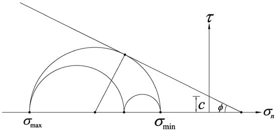
Figure 1. The Mohr-Coulomb criterion.

Letting ${\sigma }_1\ge {\sigma }_2\ge {\sigma }_3$, Equation (3) can be written as

$$({\sigma }_1-{\sigma }_3)=2c\cos \varphi -({\sigma }_1+{\sigma }_3)\sin \varphi$$

(4)

Complete yield surface can be obtained after considering all possible stress combinations. Generally, the Mohr-Coulomb yield function expressed by the invariant instead of the principal stress is used in calculation, namely

$$\sqrt{J_2}(\cos {\theta }_{\sigma }-\frac{\sin \varphi }{\sqrt{3}}\sin {\theta }_{\sigma })+\frac{1}{3}{I}_1\sin \varphi -c\cos \varphi =0-\frac{\pi }{6}\le {\theta }_{\sigma }\le \frac{\pi }{6}$$

(5)

in which

$${\theta }_{\sigma }=\frac{1}{3}{\sin }^{-1}\left[\frac{-\sqrt{27}{J}_3}{2{(J_2)}^{3/2}}\right]$$

(6)

$$J_2=\frac{1}{6}[{({\sigma }_x-{\sigma }_y)}^2+{({\sigma }_y-{\sigma }_z)}^2+{({\sigma }_z-{\sigma }_x)}^2+6({\tau }_{xy}^2+{\tau }_{yz}^2+{\tau }_{zx}^2)]$$

(7)

$$J_3=\left|\begin{array}{ccc}{\sigma }_x-{\sigma }_0& {\tau }_{xy}& {\tau }_{xz}\\ {\tau }_{yx}& {\sigma }_y-{\sigma }_0& {\tau }_{yz}\\ {\tau }_{zx}& {\tau }_{zy}& {\sigma }_z-{\sigma }_0\end{array}\right|$$

(8)

$$I_1={\sigma }_x+{\sigma }_y+{\sigma }_z$$

(9)

$${\sigma }_0=\frac{1}{3}({\sigma }_x+{\sigma }_y+{\sigma }_z)$$

(10)

According to Koiter’s law, when the Mohr-Coulomb criterion is used to calculate plastic strain, we have

$${\epsilon }^p={\displaystyle \sum _{\alpha =1}^m{\gamma }_{\alpha }}{\partial }_{\sigma }{f}_{\alpha }(\sigma )$$

(11)

Here, ${\gamma }_{\alpha }$ represents the plastic multiplier corresponding to the yield surface $\alpha$. A partial derivative of the Mohr-Coulomb yield function to stress component can be calculated based on the chain derivation rule:

$$\frac{\partial f}{\partial \sigma }=\frac{\partial f}{\partial I_1}\frac{\partial I_1}{\partial \sigma }+\frac{\partial f}{\partial J_2}\frac{\partial J_2}{\partial \sigma }+\frac{\partial f}{\partial J_3}\frac{\partial J_3}{\partial \sigma }$$

(12)

in which

$$\frac{\partial f}{\partial J_2}=\frac{1}{2\sqrt{3J_2}}\cos {\theta }_{\sigma }[\sqrt{3}(1+\tan {\theta }_{\sigma }\tan 3{\theta }_{\sigma })+\sin \varphi (\tan 3{\theta }_{\sigma }-\tan {\theta }_{\sigma })]$$

(13)

$$\frac{\partial f}{\partial J_3}=\frac{\cos {\theta }_{\sigma }}{2J_2\cos 3{\theta }_{\sigma }}(\sqrt{3}\tan {\theta }_{\sigma }+\sin \varphi )$$

(14)

As we can see, when ${\theta }_{\sigma }=\pm \frac{\pi }{6}$ (the corner of Mohr-Coulomb yield surface), $\tan 3{\theta }_{\sigma }$ and $\frac{1}{\cos 3{\theta }_{\sigma }}$ in Equations (13) and (14) are undefined, that is, singularity arises from undefined partial derivatives.

On the other hand, when the Mohr-Coulomb criterion is used for calculation, the final active yield surface at its corner is unknown. In the incremental form of the elastoplastic constitutive integral, after the strain increment is applied, whether the stress point is in elastic state or plastic loading state is judged in the form of test stress based on the following conditions:

$$\{\begin{array}{ll}{f}_{\alpha ,n+1}^{\mathrm{trial}}\le 0 \mathrm{for} \mathrm{all}& \alpha \in (1,2,\cdots ,6)\Rightarrow \mathrm{elastic} \mathrm{state}\hfill \\ f_{\alpha ,n+1}^{\mathrm{trial}}>0 \mathrm{for} \mathrm{some}& \alpha \in (1,2,\cdots ,6)\Rightarrow \mathrm{plastic} \mathrm{state}\hfill \end{array}$$

(15)

where $f_{\alpha ,n+1}^{\mathrm{trial}}$ represents the test state of yield surface $\alpha$ corresponding to the strain increment, and the specific calculation method is introduced later.

It should be noted that, if only one yield surface is activated, namely, only one $f_{\alpha ,n+1}^{\mathrm{trial}}>0$, then the yield surface is the final active yield surface, that is, $f_{\alpha ,n+1}>0$. However, when multiple yield surfaces are activated, $f_{\alpha ,n+1}^{\mathrm{trial}}>0$ cannot guarantee that the yield surface is the final active yield surface, namely, there may be $f_{\alpha ,n+1}^{\mathrm{trial}}>0$ but $f_{\alpha ,n+1}<0$. As we can see in Figure 2, N¹ and N² are the normal direction of yield surface $f_1$ and $f_2$, C_1, C₂, and C₁₂ form the corner cone of $f_1$ and $f_2$ together. When ${\sigma }_{n+1}^{\mathrm{trial}}\in C_{12}$, we have $f_{1,n+1}^{\mathrm{trial}}>0$ and $f_{2,n+1}^{\mathrm{trial}}>0$; at the same time, the plastic multiplier $\Delta {\gamma }^{\alpha }>0$,$\alpha =1,2$; therefore, the activated yield surfaces $f_1$ and $f_2$ both are the final active yield surfaces; when ${\sigma }_{n+1}^{\mathrm{trial}}\in C_1$ or ${\sigma }_{n+1}^{\mathrm{trial}}\in C_2$, although $f_{1,n+1}^{\mathrm{trial}}>0$ and $f_{2,n+1}^{\mathrm{trial}}>0$ can be obtained, it can be seen that $\Delta {\gamma }^2<0$ in C₁ and $\Delta {\gamma }^1<0$ in C₂, that is, although the activated yield surfaces are two, there is only one final active surface in the end.

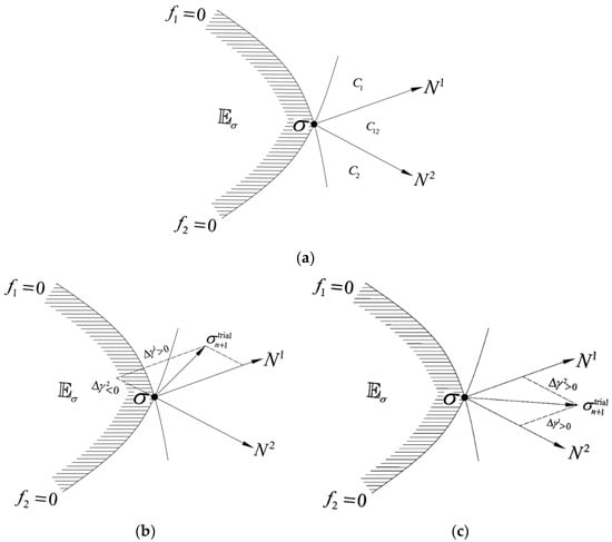
Figure 2. Geometry at a corner point. (a) definition of C₁, C₂ and C₁₂; (b) region C₁: $\Delta {\gamma }^1>0$, $\Delta {\gamma }^2<0$; (c) region C₁₂: $\Delta {\gamma }^1>0$, $\Delta {\gamma }^2>0$.

3. Algorithm and Implementation

3.1. Constitutive Integral for Mohr-Coulomb Criterion

The elastoplastic constitutive equation can be written as the following form:

$$\sigma =D(\epsilon -{\epsilon }^p)$$

(16)

Here, $\sigma$, $\epsilon$, and ${\epsilon }^p$ represent stress, strain, and plastic strain, respectively, and D is the elastic matrix. The plastic strain ${\epsilon }^p$ is determined according to Koiter’s rule in Equation (11), and the plastic multiplier satisfies the Kuhn–Tucker complementarity equation:

$$\{\begin{array}{l}{f}_{\alpha }(\sigma )\le 0\\ {\gamma }^{\alpha }\ge 0\\ {\gamma }^{\alpha }{f}_{\alpha }(\sigma )=0\end{array}$$

(17)

For the Mohr-Coulomb model with multiple yield surfaces, it is necessary to define the elastic space, which can be represented by $E_{\sigma }$ and defined as:

$$E_{\sigma }=\left\{\sigma |f_{\alpha }(\sigma )\le 0,\alpha \in [1,2,\dots ,6]\right\}$$

(18)

Furthermore, Equation (18) can be analytically written in terms of the principal stresses ${\sigma }_1$, ${\sigma }_2$, ${\sigma }_3$ as:

$$\{\begin{array}{l}{f}_1=({\sigma }_1-{\sigma }_3)+({\sigma }_1+{\sigma }_3)\sin \varphi -2c\cos \varphi \\ f_2=({\sigma }_2-{\sigma }_3)+({\sigma }_2+{\sigma }_3)\sin \varphi -2c\cos \varphi \\ f_3=({\sigma }_1-{\sigma }_2)+({\sigma }_1+{\sigma }_2)\sin \varphi -2c\cos \varphi \\ f_4=({\sigma }_3-{\sigma }_1)+({\sigma }_3+{\sigma }_1)\sin \varphi -2c\cos \varphi \\ f_5=({\sigma }_3-{\sigma }_2)+({\sigma }_3+{\sigma }_2)\sin \varphi -2c\cos \varphi \\ f_6=({\sigma }_2-{\sigma }_1)+({\sigma }_2+{\sigma }_1)\sin \varphi -2c\cos \varphi \end{array}$$

(19)

Considering a time discretization of interest, and letting $\left\{{\sigma }_n,{\epsilon }_n,{\epsilon }_n^p\right\}$ be the initial stress and strain, then, given an incremental strain $\Delta \epsilon$ and applying an implicit backward Euler difference to Equations (11) and (16), we have

$$\{\begin{array}{l}{\epsilon }_{n+1}={\epsilon }_n+\Delta \epsilon \\ {\sigma }_{n+1}=D({\epsilon }_{n+1}-{\epsilon }_{n+1}^p)\\ {\epsilon }_{n+1}^p={\epsilon }_n^p+{\displaystyle \sum \Delta {\gamma }^{\alpha }{\partial }_{\sigma }{f}_{\alpha }({\sigma }_{n+1})}\end{array}$$

(20)

Accordingly, the discrete form of Equation (17) is expressed as:

$$\{\begin{array}{l}{f}_{\alpha }({\sigma }_{n+1})\le 0\\ \Delta {\gamma }^{\alpha }\ge 0\\ \Delta {\gamma }^{\alpha }{f}_{\alpha }({\sigma }_{n+1})=0\end{array}$$

(21)

Finally, by setting $\Delta {\gamma }^{\alpha }=0$ in Equations (20) and (21), the trial state is obtained formally:

$$\{\begin{array}{l}{\epsilon }_{e,n+1}^{\mathrm{trial}}={\epsilon }_{n+1}-{\epsilon }_n^p\\ {\sigma }_{n+1}^{\mathrm{trial}}=D{\epsilon }_{e,n+1}^{\mathrm{trial}}\\ {\epsilon }_{p,n+1}^{\mathrm{trial}}={\epsilon }_n^p\\ f_{\alpha ,n+1}^{\mathrm{trial}}=f_{\alpha }({\sigma }_{n+1}^{\mathrm{trial}})\end{array}$$

(22)

A yield surface $f_{\alpha ,n+1}$ is termed active if the condition $f_{\alpha ,n+1}>0$ holds; once the trial state is obtained, an initial set of trial constraints of Mohr-Coulomb model is defined as:

$${\mathbb{J}}_{\mathrm{act}}^{\mathrm{trial}}=\left\{\alpha \in (1,2,\dots ,6)|f_{\alpha ,n+1}^{\mathrm{trial}}({\sigma }_{n+1}^{\mathrm{trial}})>0\right\}$$

(23)

If ${\mathbb{J}}_{\mathrm{act}}^{\mathrm{trial}}=\varnothing$, it indicates that it is currently in an elastic state, and the test state is the real stress state. Then, assuming plastic loading, it holds that ${\mathbb{J}}_{\mathrm{act}}^{\mathrm{trial}}\ne \varnothing$; the trial stress state ${\sigma }_{n+1}^{\mathrm{trial}}$ lays beyond the elastic region ${\mathbb{E}}_{\sigma }$ and is considered inadmissible. The solution ${\sigma }_{n+1}$ to the discrete problem can be expressed as:

$${\sigma }_{n+1}={\sigma }_n+\Delta \sigma ={\sigma }_n+D(\Delta \epsilon -\Delta {\epsilon }^p)={\sigma }_n+D\Delta \epsilon -{\displaystyle \sum _{\alpha =1}^{m}D\Delta {\gamma }^{\alpha }}{\partial }_{\sigma }{f}_{\alpha }({\sigma }_{n+1})$$

(24)

Substituting (24) into Kuhn–Tucker conditions (21), we have

$$\Delta {\gamma }^{\alpha }{f}_{\alpha }({\sigma }_n+D\Delta \epsilon -{\displaystyle \sum _{\alpha =1}^{m}D\Delta {\gamma }^{\alpha }}{\partial }_{\sigma }{f}_{\alpha }({\sigma }_{n+1}))=0$$

(25)

Equation (25) can be solved by a project contract algorithm (PCA) introduced in Section 3.3. By enforcing the Kuhn–Tucker conditions iteratively, the solution constructs a working set of constraints at each step, denoted as ${\mathbb{J}}_{\mathrm{act}}^{(k)}$. The working set of constraints is considered fixed during the iteration. It should be noted that the plastic multipliers $\Delta {\gamma }^{\alpha }$ obtained by PCA are non-negative, when all constraints $f_{n+1}^{(k)}=0$ are satisfied for $\alpha \in {\mathbb{J}}_{\mathrm{act}}^{(k)}$, admissibility of the solution is naturally satisfied, namely, $\Delta {\gamma }^{(k)}\ge 0$ for all $\alpha \in {\mathbb{J}}_{\mathrm{act}}^{(k)}$. In summary, the iteration performed on each Gauss-point proceeds by the following steps:

1

Compute elastic predictor

${\sigma }_{n+1}^{\mathrm{trial}}=D\left({\epsilon }_{n+1}-{\epsilon }_n^p\right)={\sigma }_n+D\Delta \epsilon$

$f_{\alpha ,n+1}^{\mathrm{trial}}=f_{\alpha }\left({\sigma }_{n+1}^{\mathrm{trial}}\right), for \alpha \in \left\{1,2,\dots ,6\right\}$

2

Check for plastic process

If $f_{\alpha ,n+1}^{\mathrm{trial}}\le 0$ for all $\alpha \in \left\{1,2,\dots ,6\right\}$, Set ${\sigma }_{n+1}={\sigma }_{n+1}^{\mathrm{trial}}$; ${\epsilon }_{n+1}^p={\epsilon }_n^p$, Exit

Else

$J_{\mathrm{act}}^{(0)}=\left\{\alpha \in \left\{1,2,\dots ,m\right\}|f_{\alpha ,n+1}^{\mathrm{trial}}>0\right\}$

${\epsilon }_{p,n+1}^{(0)}={\epsilon }_{p,n}$, $\Delta {\gamma }_{\alpha }^{(0)}=0$

3

Evaluate stress at iteration (k)

${\sigma }_{n+1}^{(k)}=D({\epsilon }_{n+1}-{\epsilon }_{p,n+1}^{(k)})$

4

Check convergence

$f_{\alpha ,n+1}^{(k)}=f_{\alpha }({\sigma }_{n+1}^{(k)})$, for $\alpha \in J_{\mathrm{act}}^{(k)}$

If $f_{\alpha ,n+1}^{(k)}<\mathrm{ToL}=0.1$ for all $\alpha \in J_{\mathrm{act}}^{(k)}$, Exit

Else continue

5

Computate plastic multiplier

$\Delta {\gamma }_{\alpha }^{(k)}{f}_{\alpha }\left({\sigma }_n+D\Delta \epsilon -{\displaystyle \sum _{\alpha =1}^{m}D\Delta {\gamma }_{\alpha }^{(k)}}{\partial }_{\sigma }{f}_{\alpha }({\sigma }_{n+1}^{(k)})\right)=0$

Call PCA in Section 3.3$\to \Delta {\gamma }_{\alpha }^{(k)}$

6

Update plastic strain

${\epsilon }_{p,n+1}^{(k+1)}={\epsilon }_{p,n}+{\displaystyle \sum _{\alpha =1}^m\Delta {\gamma }_{\alpha }^{(k)}}{\partial }_{\sigma }{f}_{\alpha }({\sigma }_{n+1}^{(k)})$

Set k = k + 1, Go to 3.

In elastoplastic computations using the finite element method, the load is applied incrementally. By performing the above iteration, the stress state after applying the strain increment is obtained.

3.2. Partial Derivatives of Principal Stresses with Regard to Stress Components

For Mohr-Coulomb surfaces, which have sharp corners and can be explicitly expressed in terms of principal stresses,${\sigma }_i$, i = 1, 2, and 3. While calculating plastic strains, knowing partial derivatives of principal stresses with regard to stress components will give us great convenience.

Principal stress ${\sigma }_i$ satisfies the following characteristic equation:

$${\sigma }^3-I_1{\sigma }^2-I_2\sigma -I_3=0$$

(26)

where the coefficients I₁, I₂, and I₃ are functions of the six stress components ${\sigma }_x$, ${\sigma }_y$,…, ${\tau }_{xy}$, defined as

$$I_1={\sigma }_x+{\sigma }_y+{\sigma }_z$$

(27)

$$I_2=-({\sigma }_x{\sigma }_y+{\sigma }_y{\sigma }_z+{\sigma }_z{\sigma }_x)+{\tau }_{xy}^2+{\tau }_{yz}^2+{\tau }_{zx}^2$$

(28)

$$I_3=\left|\begin{array}{ccc}{\sigma }_x& {\tau }_{xy}& {\tau }_{xz}\\ {\tau }_{yx}& {\sigma }_y& {\tau }_{yz}\\ {\tau }_{zx}& {\tau }_{zy}& {\sigma }_z\end{array}\right|$$

(29)

Differentiating Equation (26) with regard to one of ${\sigma }_x$, ${\sigma }_y$,…, ${\tau }_{xy}$, we have

$$3{\sigma }^2{\sigma }^{\prime }-I_1^{\prime }{\sigma }^2-I_1\cdot 2\sigma {\sigma }^{\prime }-I_2^{\prime }\sigma -I_2{\sigma }^{\prime }-I_3^{\prime }=0$$

(30)

with the single quote ′ associated with a quantity denoting the derivative of the quantity with regard to one of ${\sigma }_x$, ${\sigma }_y$,…, ${\tau }_{xy}$, or, equivalently,

$$(3{\sigma }^2-2I_1\sigma -I_2){\sigma }^{\prime }=I_1^{\prime }{\sigma }^2+I_2^{\prime }\sigma +I_3^{\prime }$$

(31)

Thus, we have

$${\sigma }^{\prime }=\frac{I_1^{\prime }{\sigma }^2+I_2^{\prime }\sigma +I_3^{\prime }}{3{\sigma }^2-2I_1\sigma -I_2}$$

(32)

with

• $\frac{\partial I_1}{\partial {\sigma }_x}=1$, $\frac{\partial I_1}{\partial {\tau }_{xy}}=0$, $\frac{\partial I_2}{\partial {\sigma }_x}=-\left({\sigma }_y+{\sigma }_z\right)$,
• $\frac{\partial I_2}{\partial {\tau }_{xy}}=2{\tau }_{xy}$, $\frac{\partial I_3}{\partial {\sigma }_x}={\sigma }_y{\sigma }_z-{\tau }_{yz}^2$, $\frac{\partial I_3}{\partial {\tau }_{xy}}={\tau }_{yz}{\tau }_{zx}-2{\sigma }_z{\tau }_{xy}$, etc.

Similarly, we can obtain the second derivative of the principal stress with regard to ${\sigma }_x$, ${\sigma }_y$,…, ${\tau }_{xy}$.

$${\sigma }^{″}=\frac{[4I_1^{\prime }+(2I_1-6\sigma ){\sigma }^{\prime }+2I_2^{\prime }]{\sigma }^{\prime }+I_2^{″}+I_3^{″}}{3{\sigma }^2-2I_1\sigma -I_2}$$

(33)

with

• $\frac{{\partial }^2{I}_1}{\partial {\sigma }_x^2}=0$
• $\frac{{\partial }^2{I}_2}{\partial {\sigma }_x^2}=0$,$\frac{{\partial }^2{I}_2}{\partial {\sigma }_x\partial {\sigma }_y}=-1$,$\frac{{\partial }^2{I}_2}{\partial {\tau }_{xy}^2}=2$,$\frac{{\partial }^2{I}_2}{\partial {\tau }_{xy}\partial {\tau }_{yz}}=0$
• $\frac{{\partial }^2{I}_3}{\partial {\sigma }_x^2}=0$,$\frac{{\partial }^2{I}_3}{\partial {\sigma }_x\partial {\sigma }_y}={\sigma }_z$,$\frac{{\partial }^2{I}_3}{\partial {\sigma }_x\partial {\tau }_{yz}}=-2{\tau }_{yz}$,$\frac{{\partial }^2{I}_3}{\partial {\tau }_{xy}^2}=-2{\sigma }_z$,$\frac{{\partial }^2{J}_3}{\partial {\tau }_{xy}\partial {\tau }_{yz}}={\tau }_{zx}$, etc.

3.3. Algorithm PCA

Given a subset K of Euclidean n-dimensional space $R^n$ and a mapping $F:K\to R^n$, the variational inequality finds a vector $x\in K$ such that

$${(y-x)}^{T}F(x)\ge 0, \forall y\in K$$

(34)

Given a mapping $F:R_{+}^n\to R^n$, the nonlinear complementarity problem is to find a vector $x\in R^n$ satisfying

$$0\le x\perp F(x)\ge 0$$

(35)

In fact, when the subset K in the variational inequality is non-negative, the nonlinear complementarity problem is equivalent to the variational inequality [21]. As a method for solving convex optimization problems under the framework of variational inequalities, just as the name implies, the projection contraction algorithm is a contraction algorithm based on projection. Here, we only refer to the algorithm part; for more details, see [22].

Rewrite complementary equation system (21) to vector form:

$$0\le \Delta \mathit{\gamma }\perp \mathit{F}(\Delta \mathit{\gamma })\ge 0$$

(36)

in which $\Delta \mathit{\gamma }=(\Delta {\gamma }_1,\dots ,\Delta {\gamma }_m)$, $\mathit{F}(\Delta \mathit{\gamma })=(-f_1(\Delta {\gamma }_1),\dots ,-f_m(\Delta {\gamma }_m))$. As we can see from Equation (35), the complementary system in (36) can be summarized as a typical nonlinear complementarity problem, which can be solved by the projection contraction method.

The projection contraction algorithm (PCA) is invoked in this way:

$$(\Delta \mathit{\gamma })=PCA(\Delta {\mathit{\gamma }}^0,F)$$

(37)

The input arguments of $\Delta {\mathit{\gamma }}^0$ is the initial guess of plastic multiplier $\Delta \mathit{\gamma }$. In general, $\Delta {\mathit{\gamma }}^0$ = 0.

The pseudocode of PCA is listed as follows, and He proposed [22] three parameters in PCA as $\xi$ = 0.9, $\eta$ = 0.4, and $\lambda$ = 1.9, which is also adopted in this paper. It should be noted that the parameters have little effect on the result.

Step 0: Let step size $\beta$ = 1; $k$ = 0; error tolerance $\epsilon =0.1\%$

Step 1: $\mathit{F}=\mathit{F}\mathit{A}\left(\Delta \mathit{\gamma }\right); \Delta \tilde{\mathit{\gamma }}=\max \left[\Delta \mathit{\gamma }-\beta \mathit{F},0\right]$

$\mathit{d}\left(\Delta \mathit{\gamma },\Delta \tilde{\mathit{\gamma }}\right)=\Delta \mathit{\gamma }-\Delta \tilde{\mathit{\gamma }}$

if $\Vert \mathit{d}\left(\Delta \mathit{\gamma },\Delta \tilde{\mathit{\gamma }}\right)\Vert \le \epsilon$ then $\Delta \mathit{\gamma }=\Delta \tilde{\mathit{\gamma }}$; break

$\tilde{\mathit{F}}=\mathit{F}\mathit{A}\left(\Delta \tilde{\mathit{\gamma }}\right)$; $\mathit{F}\left(\Delta \mathit{\gamma },\Delta \tilde{\mathit{\gamma }}\right)=\mathit{F}-\tilde{\mathit{F}}$; $r=\frac{\beta {\Vert \mathit{F}\left(\Delta \mathit{\gamma },\Delta \tilde{\mathit{\gamma }}\right)\Vert }_2}{{\Vert \mathit{d}\left(\Delta \mathit{\gamma },\Delta \tilde{\mathit{\gamma }}\right)\Vert }_2}$;

while $r>\xi$

$\beta =0.7*\beta *\min \left(1,\frac{1}{r}\right)$; $\Delta \tilde{\mathit{\gamma }}=\max \left[\Delta \mathit{\gamma }-\beta \mathit{F},0\right]$; $\tilde{\mathit{F}}=\mathit{F}\mathit{A}(\Delta \tilde{\mathit{\gamma }})$;

$\mathit{F}\left(\Delta \mathit{\gamma },\Delta \tilde{\mathit{\gamma }}\right)=\mathit{F}-\tilde{\mathit{F}}$; $\mathit{d}\left(\Delta \mathit{\gamma },\Delta \tilde{\mathit{\gamma }}\right)=\Delta \mathit{\gamma }-\Delta \tilde{\mathit{\gamma }}$; $r=\frac{\beta {\Vert \mathit{F}\left(\Delta \mathit{\gamma },\Delta \tilde{\mathit{\gamma }}\right)\Vert }_2}{{\Vert \mathit{d}\left(\Delta \mathit{\gamma },\Delta \tilde{\mathit{\gamma }}\right)\Vert }_2}$;

end(while)

$\mathit{D}\left(\Delta \mathit{\gamma },\Delta \tilde{\mathit{\gamma }}\right)=\mathit{d}\left(\Delta \mathit{\gamma },\Delta \tilde{\mathit{\gamma }}\right)-\beta \mathit{F}\left(\Delta \mathit{\gamma },\Delta \tilde{\mathit{\gamma }}\right)$; $\alpha =\frac{{\left[\mathit{d}\left(\Delta \mathit{\gamma },\Delta \tilde{\mathit{\gamma }}\right)\right]}^T\mathit{D}\left(\Delta \mathit{\gamma },\Delta \tilde{\mathit{\gamma }}\right)}{{\Vert \mathit{D}\left(\Delta \mathit{\gamma },\Delta \tilde{\mathit{\gamma }}\right)\Vert }_2^2}$;

$\Delta \mathit{\gamma }=\Delta \mathit{\gamma }-\lambda \alpha \mathit{d}\left(\Delta \mathit{\gamma },\Delta \tilde{\mathit{\gamma }}\right)$;

if $r\le \eta$ then $\beta =1.5*\beta$;

Step 2. k = k + 1; go to Step 1.

4. Numerical Examples

The practical application of the proposed algorithm is illustrated in this section by two different numerical examples. For all the examples, four node isoparametric elements with four Gaussian points are adopted, and the error tolerance for unbalanced force in the equilibrium iteration is 0.1%.

4.1. Strip Footing Collapse

The bearing capacity of a strip footing is calculated under undrained conditions by the proposed method. The soil is assumed weightless, isotropic, and is modeled as a Mohr-Coulomb perfectly plastic material. There is no friction at the footing/soil interface. The computational model and discretized mesh are shown in Figure 3. The material parameters are assumed as follows: Young’s modulus: E = 107 MPa, Poisson’s ratio: v = 0.48, cohesion c = 490 kPa, and internal friction angle $\varphi ={20}^{°}$. A plane strain state is assumed.

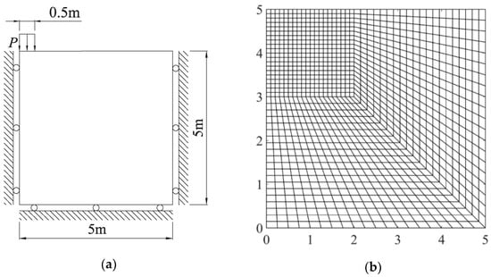
Figure 3. Strip footing: (a) problem geometry; (b) adopted mesh.

The strip footing is subjected to a vertical pressure P and the aim of present analysis is to obtain the limit pressure P_lim. A solution to this problem has been derived by Prandtl and Hill [23]:

$$P_{\lim }=c\left[e^{\pi \tan \phi }{\tan }^2({45}^{°}+\frac{\phi }{2})-1\right]\cot \phi$$

(38)

The pressure P is increased incrementally to failure and corresponding load/settlement (average) curves obtained are plotted in Figure 4.

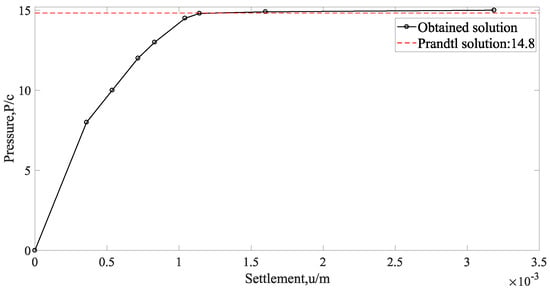
Figure 4. Pressure versus displacement.

The limit loads obtained are

$$\frac{P_{\lim }^N}{c}\approx 15$$

(39)

This value is in good agreement with Prandtl’s solution (1.2% above)

$$\frac{P_{\lim }}{c}\approx 14.82$$

(40)

The equivalent plastic strain at the failure load is shown in Figure 5. As we can see from Figure 5, at the moment that the foundation enters flow, the global shear failure of the foundation develops downward to a certain depth and extends to the ground The failure mechanism captured in the finite element analysis is in good agreement with the slip-line field of strip footing as shown in Figure 6 [24].

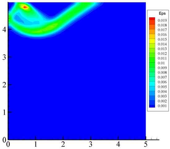
Figure 5. Equivalent plastic strain at the failure load.

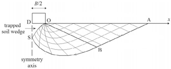
Figure 6. Slip-line field of strip footing.

4.2. Slope Stability

In this example, the plane strain analysis of a slope subjected to self-weight is carried out. To assess the safety of the slope shown in Figure 7, the strength reduction method is adopted. Table 1 lists the mechanical parameters. The materials comply with the perfectly Mohr-Coulomb criterion. Horizontal displacements are fixed for nodes along the left and right boundaries while both horizontal and vertical displacements are fixed along the bottom boundary.

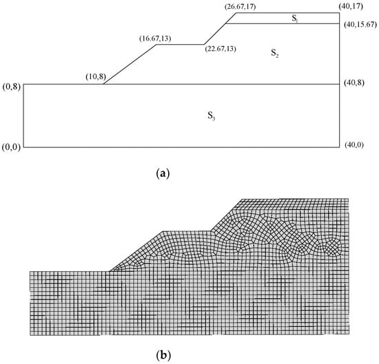
Figure 7. Slope stability: (a) problem geometry; (b) adopted mesh.

Table 1. Parameters for soil.

Soil	$\mathit{\gamma }(\mathbf{kN}/{\mathbf{m}}^3)$	$\mathit{E}(\mathbf{MPa})$	$\mathit{\nu }$	$\mathit{c}(\mathbf{kPa})$	$\mathit{\varphi }(°)$
S1	18	4	0.4	10	13.6
S2	19.2	4	0.38	20.8	15.1
S3	17.5	35	0.42	16.1	9.3

For slopes, the factor of safety Fs is traditionally defined as the ratio of the actual shear strength to the minimum shear strength required to prevent failure. An obvious way of computing Fs with a finite element or a finite difference program is simply to reduce the shear strength until collapse occurs. This technique was used as early as 1975 by Zienkiewicz et al. [25], and has since been applied by Naylor [26], Matsui and San [27], Ugai and Leschinsky [28], Dawson et al. [29], and many others. There are a variety of criteria of the limit equilibrium state, see [30]. The differences of the factors of safety based on different criteria are small.

The initial reduction factor is set as 1, then increases gradually until the slope collapse. It is noteworthy that Young’s modulus E and Poission’s ratio, v are rectified based on [31] while using the strength reduction technique.

The horizontal displacement at the top corner of the slope with the reduction factor is shown in Figure 8; when the reduction factor F = 1.35, there is an obvious inflection point on the displacement curve. At this time, the distribution of the plastic zone is shown in Figure 9, the plastic zone is just go-through.

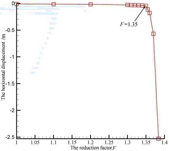
Figure 8. The horizontal displacement versus reduction factor.

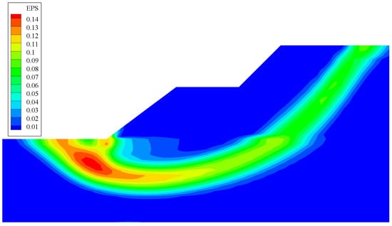
Figure 9. Distribution of equivalent plastic strain at the top corner of the slope.

If the reduction factor at the inflection point is taken as the safety factor, then Fs = 1.35; if the reduction factor when the calculation fails to converge is taken as the safety factor, then Fs = 1.38. The gap between the two results is very small. Figure 9 shows that, once an earth slope is led to the limit equilibrium state by means of the strength reduction technique, a plastic zone will go through the slope from the toe to the top.

The slope safety factor obtained by Spencer is Fs = 1.33, and the corresponding critical slip surface is shown in Figure 10, in which green line represents the slip surface and three colors top-down represents different soils in Table 1; due to the obeservation that the critical slip surface within the plastic zone will consist of the points at which the equivalent plastic strain takes the local maximum in the vertical direction [32], we can see that the obtained critical sliding surface by the Spencer method is in good agreement with the failure mechanism shown in Figure 9.

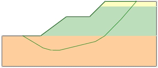
Figure 10. The critical slip surface of Spencer.

A comparison about computational efficiency is made between the PCA and the classic mapping return method in [17]. Integral points that are undergoing plastic deformation are selected. A comparison is made based on the computation time for 10,000 stress returns, and is implemented in Matlab on a computer with Intel(R) Core(TM) i5-3230M 2.60 GHz processor. Table 2 lists the results.

Table 2. Comparison of time spending.

Number of Activated Surface	Time (Classic)	Time (Present)	Ratio
1	1.692	1.373	1.232
2	2.438	1.464	1.665

It can be seen that the present PCA is substantially more efficient than the classic mapping return method, especially when more than one yield surface is ever activated.

5. Conclusions

Based on the complementarity theory, the elasto-plastic complementarity equation is established. The corner problems of multiple surfaces are unified into a set of complementary equations by using Koiter’s law, and then solved by using the projection contraction algorithm. The theory and examples show that: the projection contraction algorithm for the complementary equation with multiple yield surfaces avoids the accuracy and convergence problems caused by corner smoothing; the stress return operation is carried out in the general stress space, and the partial derivative of the corresponding stress component is calculated in the principal stress space, which not only avoids the numerical singularity at the corner, but also eliminates the stress transformation of the stress return in the principal stress space.

References

- Koiter, W.T. Stress-strain relations, uniqueness and variational theorems for elastic-plastic materials with a singular yield surface. Q. Appl. Math. 1953, 11, 350–354. [Google Scholar] [CrossRef]
- Zienkiewicz, O.C.; Valliappan, S.; King, I.P. Elasto-plastic solutions of engineering problems ‘initial stress’, finite element approach. Int. J. Numer. Methods Eng. 1969, 1, 75–100. [Google Scholar] [CrossRef]
- Hinton, E.; Owen, D.R.J. Finite Elements in Plasticity: Theory and Practice; Pineridge Press: Swansea, UK, 1980; pp. 20–45. [Google Scholar]
- Marques, J. Stress computation in elastoplasticity. Eng. Comput. 1984, 1, 42–51. [Google Scholar] [CrossRef]
- Zienkiewicz, O.C.; Pande, G.N. Some useful forms for isotropic yield surfaces for soils and rock mechanics. In Finite Elements in Geomechanics; Gudehus, G., Ed.; John Wiley & Sons: Hoboken, NJ, USA, 1977; pp. 179–190. [Google Scholar]
- Sloan, S.W.; Booker, J.R. Removal of singularities in tresca and Mohr-Coulomb yield functions. Commun. Appl. Numer. Methods 1986, 2, 173–179. [Google Scholar] [CrossRef]
- Abbo, A.; Lyamin, A.; Sloan, S.; Hambleton, J. A C2 continuous approximation to the Mohr–Coulomb yield surface. Int. J. Solids Struct. 2011, 48, 3001–3010. [Google Scholar] [CrossRef]
- Larsson, R.; Runesson, K. Implicit integration and consistent linearization for yield criteria of the Mohr-Coulomb type. Mech. Cohesive -Frict. Mater. 1996, 1, 367–383. [Google Scholar] [CrossRef]
- Peric, D.; Neto, E.D.S. A new computational model for Tresca plasticity at finite strains with an optimal parametrization in the principal space. Comput. Methods Appl. Mech. Eng. 1999, 171, 463–489. [Google Scholar] [CrossRef]
- Neto, E.A.D.S.; Peri, D.; Owen, D.R.J. Computational Methods for Plasticity: Theory and Applications; John Wiley & Sons: Hoboken, NJ, USA, 2008. [Google Scholar] [CrossRef]
- de Borst, R. Integration of plasticity equations for singular yield functions. Comput. Struct. 1987, 26, 823–829. [Google Scholar] [CrossRef][Green Version]
- Pankaj, P.; Bićanić, N. Detection of multiple active yield conditions for Mohr-Coulomb elasto-plasticity. Comput. Struct. 1997, 62, 51–61. [Google Scholar] [CrossRef]
- Clausen, J.; Damkilde, L.; Andersen, L. An efficient return algorithm for non-associated plasticity with linear yield criteria in principal stress space. Comput. Struct. 2007, 85, 1795–1807. [Google Scholar] [CrossRef]
- Coombs, W.M.; Crouch, R.S.; Augarde, C.E. Reuleaux plasticity: Analytical backward Euler stress integration and consistent tangent. Comput. Methods Appl. Mech. Eng. 2010, 199, 1733–1743. [Google Scholar] [CrossRef][Green Version]
- Amouzou, G.; Soulaïmani, A. Numerical Algorithms for Elastoplacity: Finite Elements Code Development and Implementation of the Mohr–Coulomb Law. Appl. Sci. 2021, 11, 4637. [Google Scholar] [CrossRef]
- Zhao, R.; Li, C.; Zhou, L.; Zheng, H. A sequential linear complementarity problem for multisurface plasticity. Appl. Math. Model. 2021, 103, 557–579. [Google Scholar] [CrossRef]
- Simo, J.C.; Kennedy, J.G.; Govindjee, S. Non-smooth multisurface plasticity and viscoplasticity. Loading/unloading conditions and numerical algorithms. Int. J. Numer. Methods Eng. 1988, 26, 2161–2185. [Google Scholar] [CrossRef]
- Karaoulanis, F.E. Implicit Numerical Integration of Nonsmooth Multisurface Yield Criteria in the Principal Stress Space. Arch. Comput. Methods Eng. 2013, 20, 263–308. [Google Scholar] [CrossRef]
- Clausen, J.; Damkilde, L. An exact implementation of the Hoek–Brown criterion for elasto-plastic finite element calculations. Int. J. Rock Mech. Min. Sci. 2008, 45, 831–847. [Google Scholar] [CrossRef]
- Adhikary, D.P.; Jayasundara, C.T.; Podgorney, R.K.; Wilkins, A.H. A robust return-map algorithm for general multisurface plasticity. Int. J. Numer. Methods Eng. 2017, 109, 218–234. [Google Scholar] [CrossRef]
- Facchinei, F.; Pang, J.-S. Finite-Dimensional Variational Inequalities and Complementarity Problems; Springer: Berlin/Heidelberg, Germany, 2004. [Google Scholar] [CrossRef]
- He, B. A Class of Projection and Contraction Methods for Monotone Variational Inequalities. Appl. Math. Optim. 1997, 35, 69–76. [Google Scholar] [CrossRef]
- Hill, R. The Mathematical Theory of Plasticity; Oxford University Press: London, UK, 1950; pp. 253–260. [Google Scholar]
- Vo, T.; Russell, A.R. Bearing capacity of strip footings on unsaturated soils by the slip line theory. Comput. Geotech. 2015, 74, 122–131. [Google Scholar] [CrossRef]
- Zienkiewicz, O.C.; Humpheson, C.; Lewis, R.W. Associated and nonassociated viscoplasticity in soil mechanics. Géotechnique 1975, 25, 671–689. [Google Scholar] [CrossRef]
- Naylor, D.J. Finite elements and slope stability. In Numerical Methods in Geomechanics; Springer: Dordrecht, The Netherland, 1981; pp. 229–244. [Google Scholar]
- Matsui, T.; San, K.-C. Finite Element Slope Stability Analysis by Shear Strength Reduction Technique. Soils Found. 1992, 32, 59–70. [Google Scholar] [CrossRef]
- Ugai, K.; Leshchinsky, D. Three-Dimensional Limit Equilibrium and Finite Element Analyses: A Comparison of Results. Soils Found. 1995, 35, 1–7. [Google Scholar] [CrossRef]
- Dawson, E.M.; Roth, W.H.; Drescher, A. Slope stability analysis by strength reduction. Géotechnique 1999, 49, 835–840. [Google Scholar] [CrossRef]
- Griffiths, D.V.; Lane, P.A. Slope stability analysis by finite elements. Géotechnique 1999, 49, 387–403. [Google Scholar] [CrossRef]
- Zheng, H.; Liu, D.F.; Li, C.G. Slope stability analysis based on elasto-plastic finite element method. Int. J. Numer. Methods Eng. 2005, 64, 1871–1888. [Google Scholar] [CrossRef]
- Zheng, H.; Sun, G.; Liu, D. A practical procedure for searching critical slip surfaces of slopes based on the strength reduction technique. Comput. Geotech. 2009, 16, 1–5. [Google Scholar] [CrossRef]
Publisher’s Note: MDPI stays neutral with regard to jurisdictional claims in published maps and institutional affiliations. |
© 2022 by the authors. Licensee MDPI, Basel, Switzerland. This article is an open access article distributed under the terms and conditions of the Creative Commons Attribution (CC BY) license (https://creativecommons.org/licenses/by/4.0/).