


Assessment of Bayesian Changepoint Detection Methods for Soil Layering Identification Using Cone Penetration Test Data


Abstract
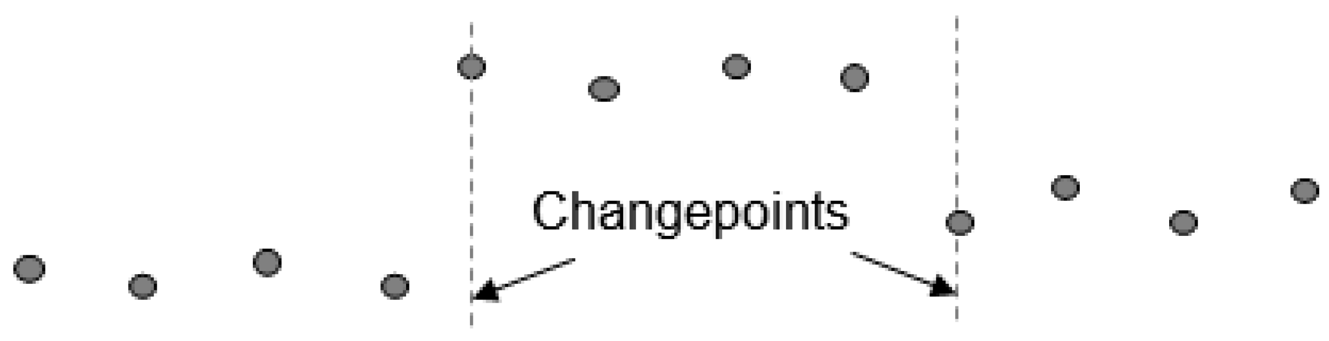
1. Introduction
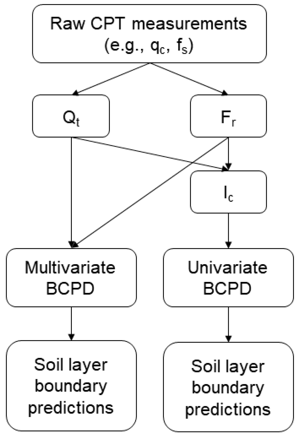
2. Methodology
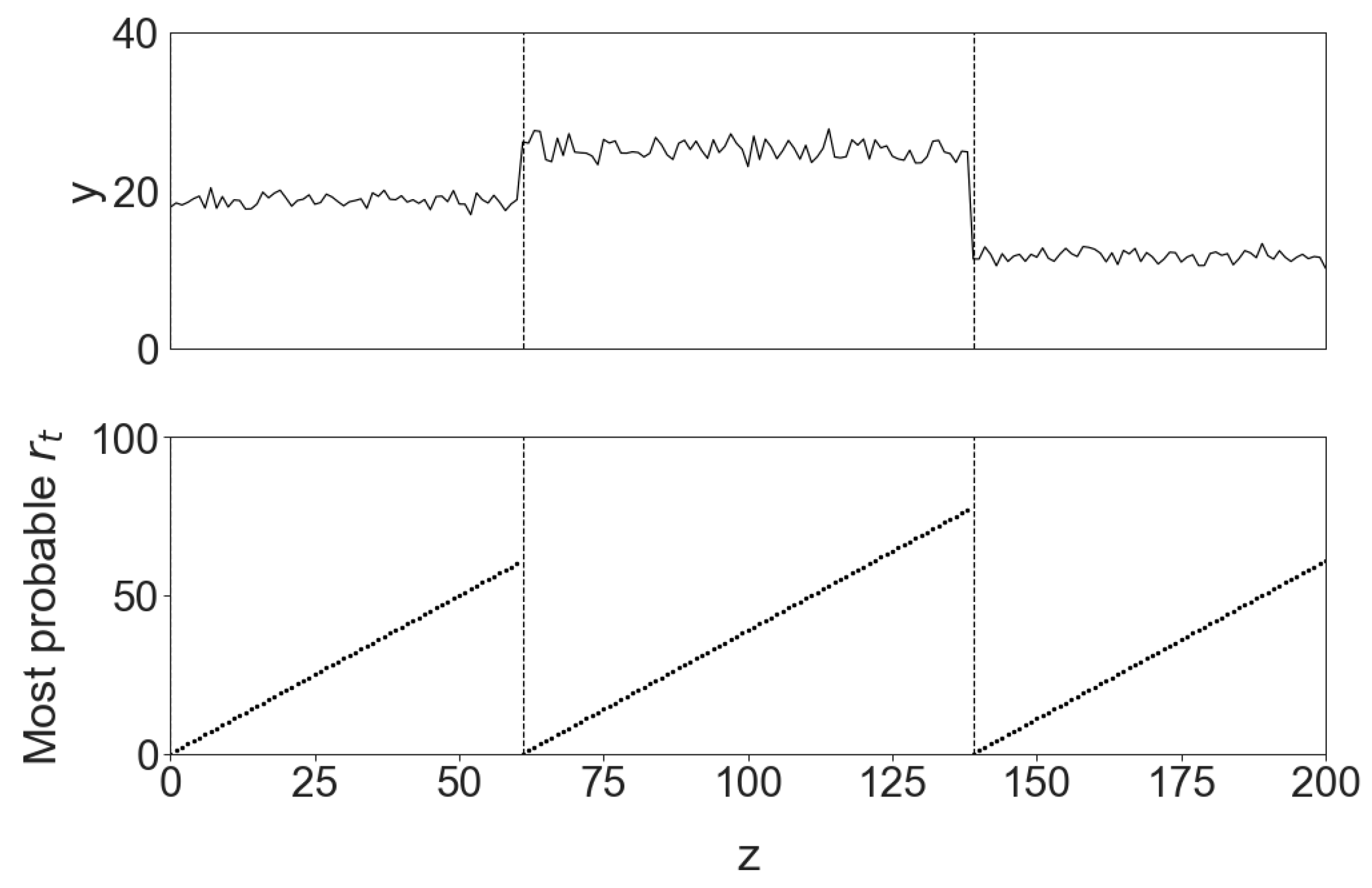
2.1. Offline BCPD
Maximum a Posteriori Estimations of Changepoints
2.2. Online BCPD
Maximum a Posteriori Estimations of Changepoints
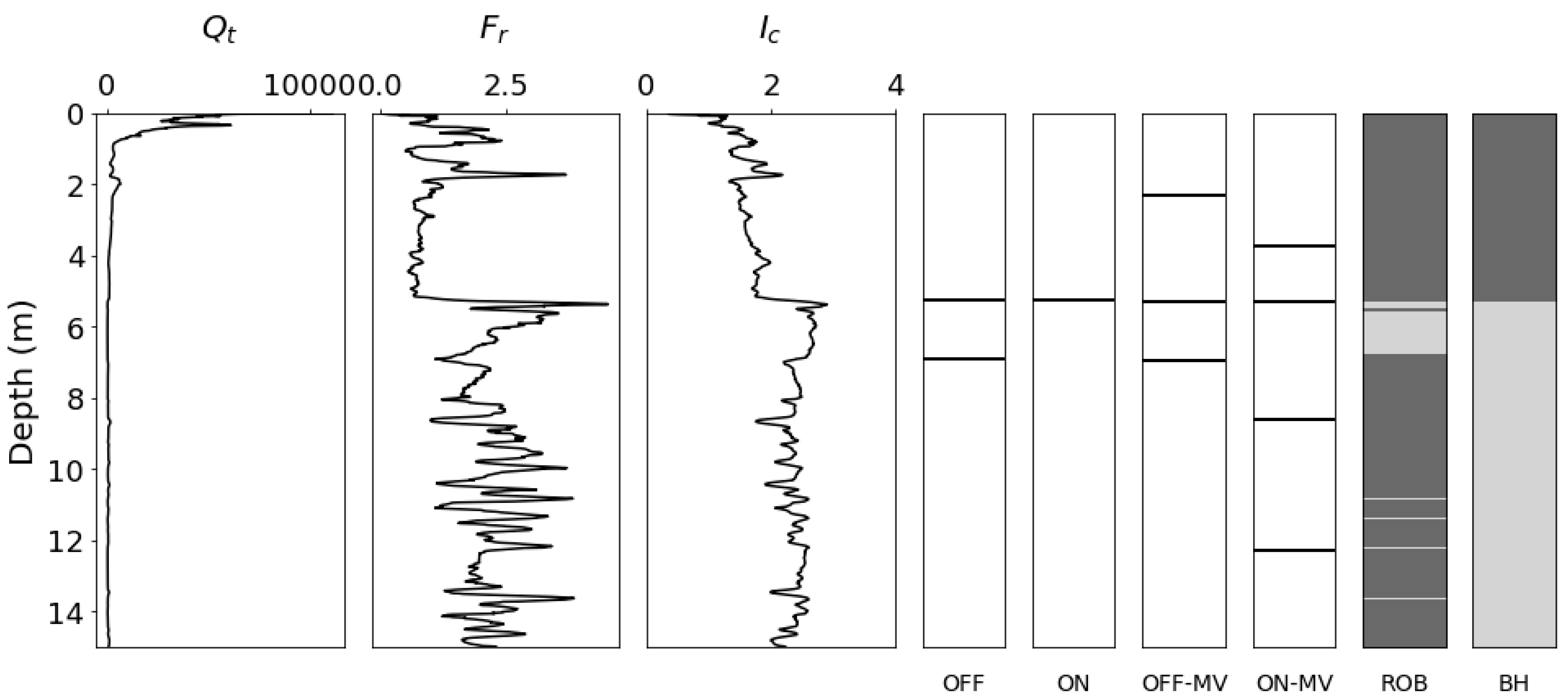
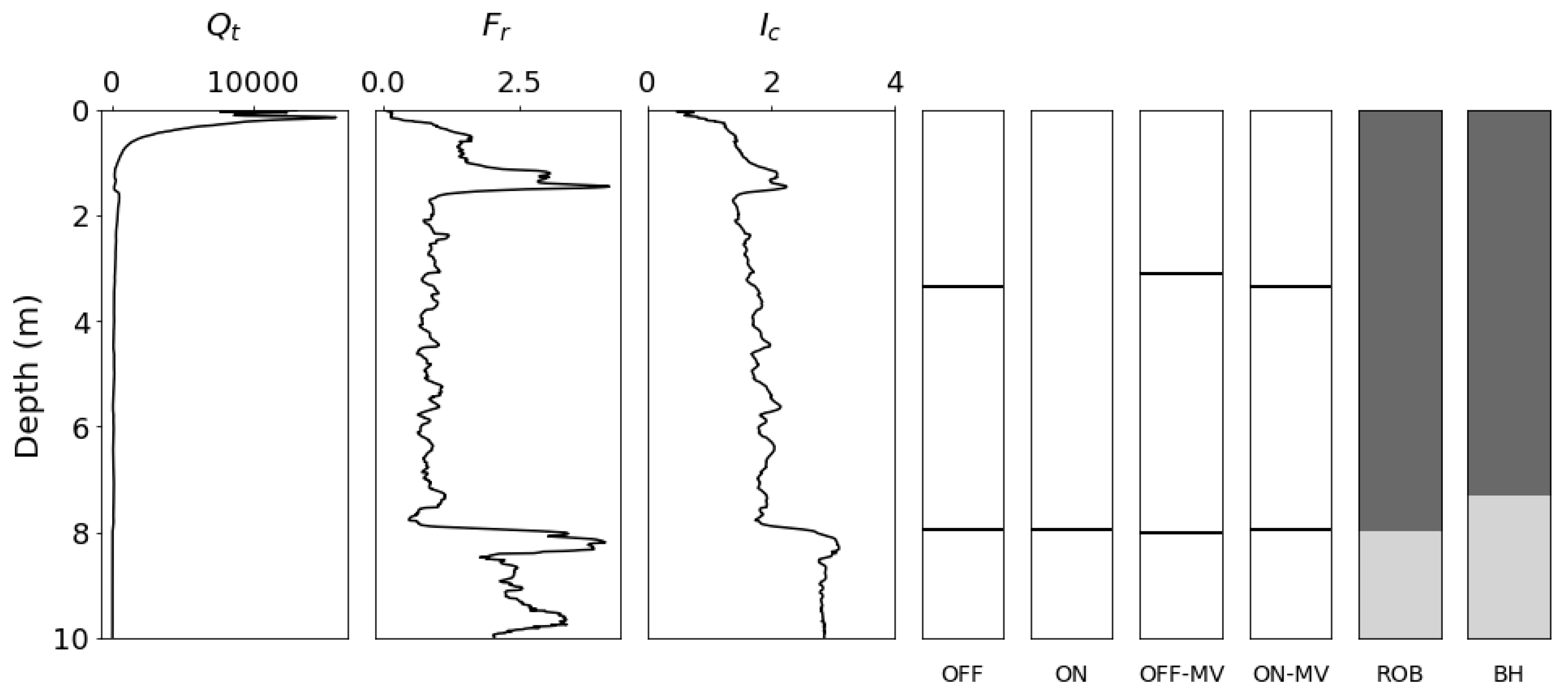
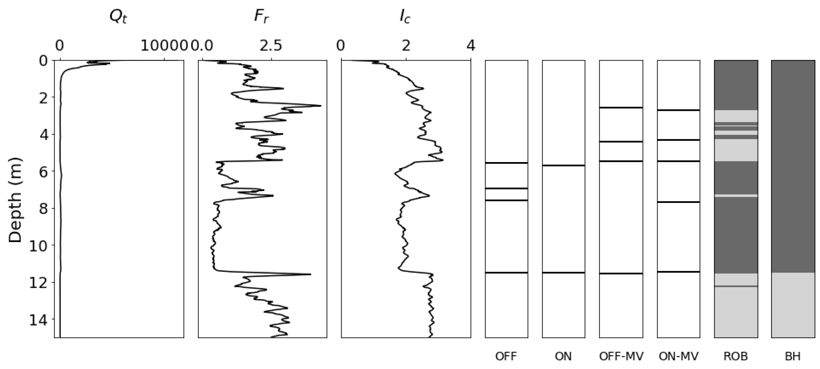
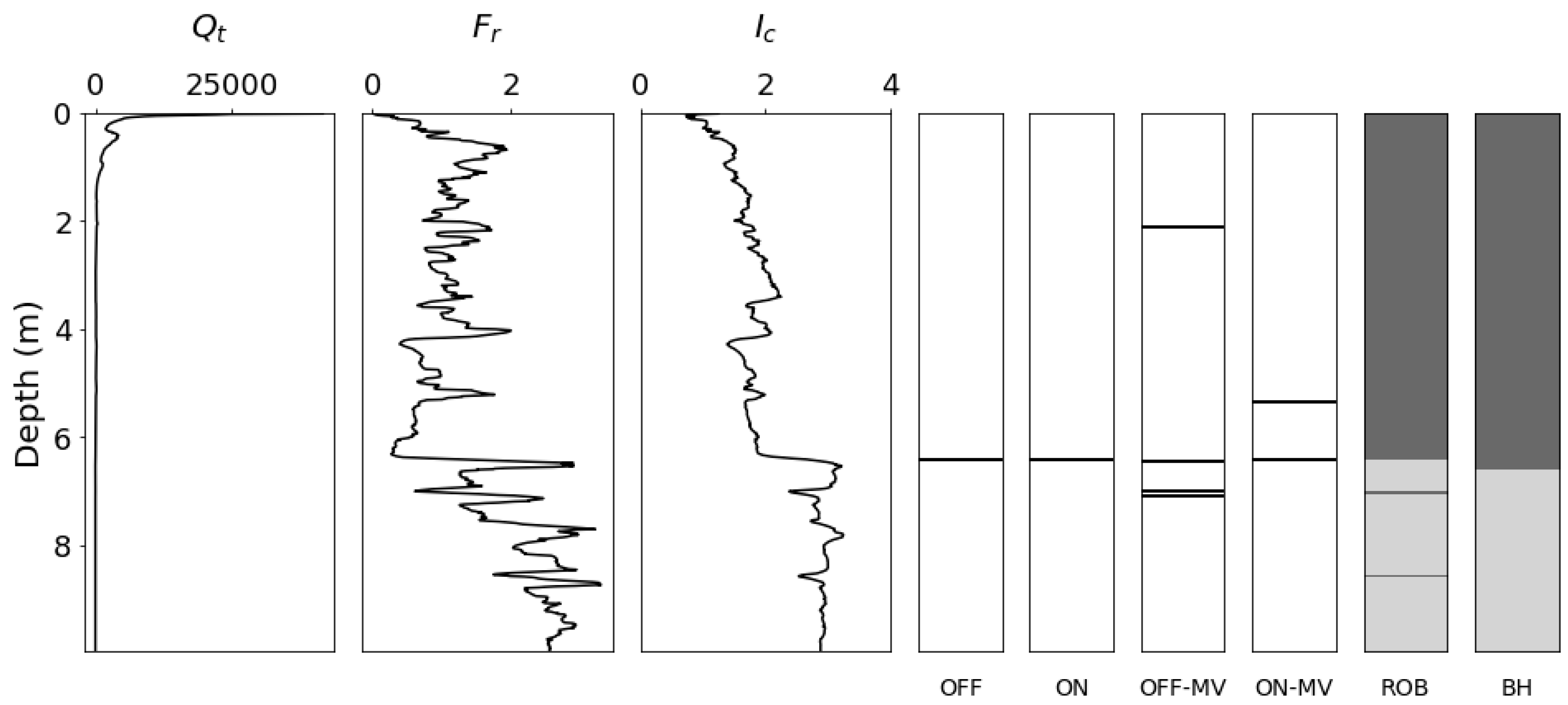
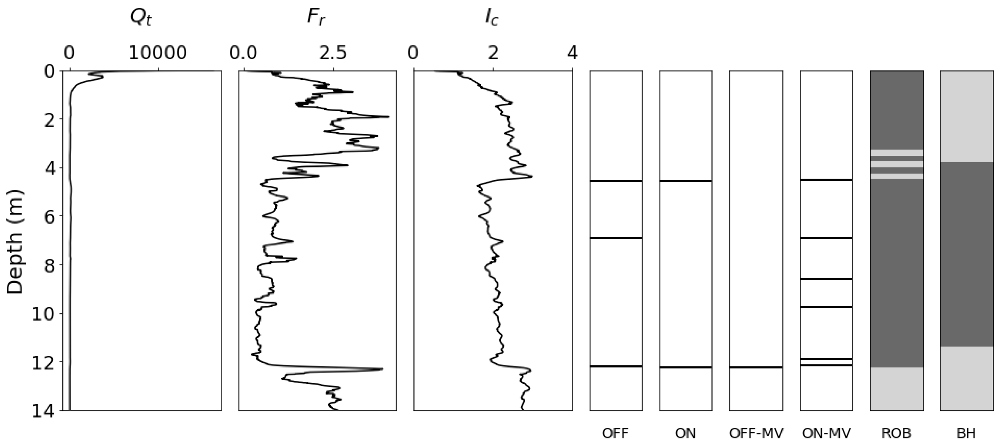
2.3. CPT Data Case Study
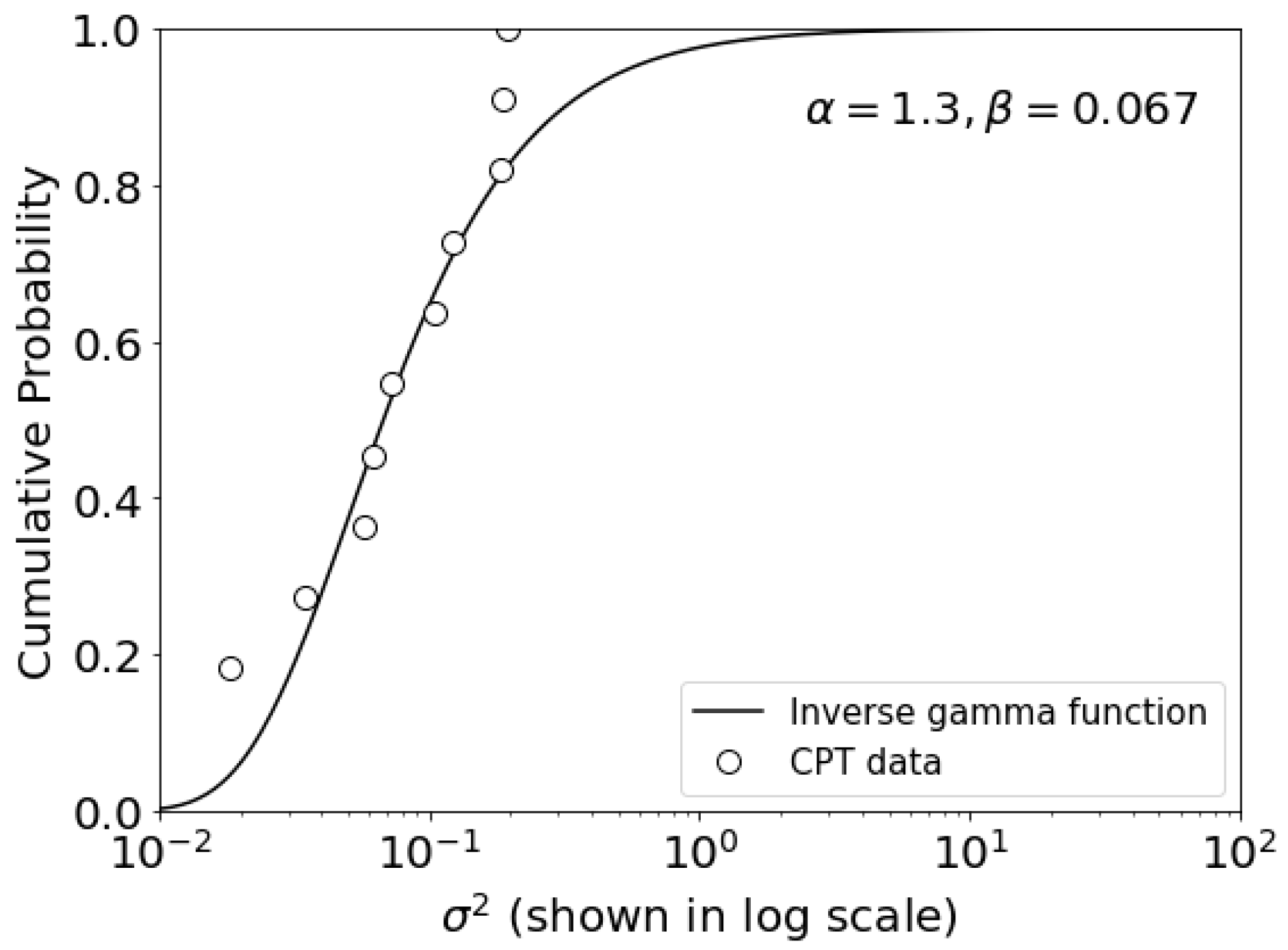
2.4. Priors for Univariate and Multivariate BCPD Methods
2.5. Performance Metrics
- True Positive (TP)—the number of times the method has correctly identified a soil layer boundary;
- False Positive (FP)—the number of times the method has incorrectly identified a soil layer boundary;
- False Negative (FN)—the number of times the method has failed to identify a true soil layer boundary;
- Precision = TP/(TP + FP);
- Sensitivity = TP/(TP + FN);
- F1 score = 2(Precision × Sensitivity)/(Precision + Sensitivity).
3. Results
Comparison of Performance Metrics
4. Discussion
5. Conclusions
- Univariate BCPD methods (using data) are generally more accurate and computationally efficient than their multivariate counterparts (using and data) in identifying soil layer boundaries using CPT data.
- The newly developed univariate online BCPD method demonstrates the highest accuracy and computational efficiency.
- This research underscores the advantage of unsupervised BCPD methods, which forego the need for training data and manual analysis, contributing to the advancement of fast, automated Bayesian geotechnical analysis techniques.
Author Contributions
Funding
Data Availability Statement
Acknowledgments
Conflicts of Interest
References
- Suryasentana, S.K.; Mayne, P.W. Simplified method for the lateral, rotational, and torsional static stiffness of circular footings on a nonhomogeneous elastic half-space based on a work-equivalent framework. J. Geotech. Geoenviron. Eng. 2022, 148, 04021182. [Google Scholar] [CrossRef]
- Mayne, P.W.; Poulos, H.G. Approximate displacement influence factors for elastic shallow foundations. J. Geotech. Geoenviron. Eng. 1999, 125, 453–460. [Google Scholar] [CrossRef]
- Gupta, B.K.; Basu, D. Offshore wind turbine monopile foundations: Design perspectives. Ocean Eng. 2020, 213, 107514. [Google Scholar] [CrossRef]
- Doherty, P.; Gavin, K. Laterally loaded monopile design for offshore wind farms. Proc. Inst. Civ. Eng. 2012, 165, 7–17. [Google Scholar] [CrossRef]
- Byrne, B.W.; Houlsby, G.T.; Burd, H.J.; Gavin, K.G.; Igoe, D.J.; Jardine, R.J.; Martin, C.M.; McAdam, R.A.; Potts, D.M.; Taborda, D.M.; et al. PISA design model for monopiles for offshore wind turbines: Application to a stiff glacial clay till. Géotechnique 2020, 70, 1030–1047. [Google Scholar] [CrossRef]
- Byrne, B.W.; Aghakouchak, A.; Buckley, R.M.; Burd, H.J.; Gengenbach, J.; Houlsby, G.T.; McAdam, R.A.; Martin, C.M.; Schranz, F.; Sheil, B.B.; et al. PICASO: Cyclic lateral loading of offshore wind turbine monopiles. In Proceedings of the 4th International Symposium on Frontiers in Offshore Geotechnics (ISFOG 2021), Austin, TX, USA, 8–11 November 2021. [Google Scholar]
- Houlsby, G.T.; Ibsen, L.B.; Byrne, B.W. Suction caissons for wind turbines. In Frontiers in Offshore Geotechnics; ISFOG: Perth, WA, Australia, 2005; pp. 75–93. [Google Scholar]
- Byrne, B.; Houlsby, G.; Martin, C.; Fish, P. Suction caisson foundations for offshore wind turbines. Wind. Eng. 2002, 26, 145–155. [Google Scholar] [CrossRef]
- Suryasentana, S.K.; Byrne, B.W.; Burd, H.J.; Shonberg, A. Simplified model for the stiffness of suction caisson foundations under 6DoF loading. In Proceedings of the SUT OSIG 8th International Conference 2017, London, UK, 12–14 September 2017; pp. 554–561. [Google Scholar]
- Suryasentana, S.K.; Byrne, B.W.; Burd, H.J.; Shonberg, A. An elastoplastic 1D Winkler model for suction caisson foundations under combined loading. In Numerical Methods in Geotechnical Engineering IX; CRC Press: Boca Raton, FL, USA, 2018; pp. 973–980. [Google Scholar]
- Suryasentana, S.K.; Burd, H.J.; Byrne, B.W.; Shonberg, A. Modulus weighting method for stiffness estimations of suction caissons in layered soils. Géotech. Lett. 2023, 13, 97–104. [Google Scholar] [CrossRef]
- Lunne, T.; Robertson, P.K.; Powell, J.J.M. Cone Penetration Testing in Geotechnical Practice; Blackie Academic and Professional: London, UK, 1997. [Google Scholar]
- Jamiolkowski, M.; Ghionna, V.N.; Lancellotta, R.; Pasqualini, E. New correlations of penetration tests for design practice: Proc 1st International Symposium on Penetration Testing, ISOPT-1, Orlando, 20–24 March 1988V1, P263–296. Rotterdam: A A Balkema, 1988. Int. J. Rock Mech. Min. Sci. Geomech. Abstr. 1990, 27, A91. [Google Scholar] [CrossRef]
- Sakleshpur, V.A.; Prezzi, M.; Salgado, R.; Zaheer, M. CPT-Based Geotechnical Design Manual, Volume 2: CPT-Based Design of Foundations—Methods (Joint Transportation Research Program Publication No. FHWA/IN/JTRP2021/23); Purdue University: West Lafayette, IN, USA, 2021. [Google Scholar] [CrossRef]
- Suryasentana, S.K.; Lehane, B.M. Verification of numerically derived CPT based py curves for piles in sand. In Proceedings of the 3rd International Symposium on Cone Penetration Testing, Las Vegas, NV, USA, 13–14 May 2014; pp. 3–29. [Google Scholar]
- Robertson, P.K. Soil classification using the cone penetration test. Can. Geotech. J. 1990, 27, 151–158. [Google Scholar] [CrossRef]
- Robertson, P.K.; Wride, C.E. Evaluating cyclic liquefaction potential using the cone penetration test. Can. Geotech. J. 1998, 35, 442–459. [Google Scholar] [CrossRef]
- Robertson, P.K. Interpretation of cone penetration tests—A unified approach. Can. Geotech. J. 2009, 46, 1337–1355. [Google Scholar] [CrossRef]
- Robertson, P.K. Soil behaviour type from the CPT: An update. In Proceedings of the 2nd International Symposium on Cone Penetration Testing, Huntington Beach, CA, USA, 9–11 May 2010; Cone Penetration Testing Organizing Committee: Huntington Beach, CA, USA, 2010; Volume 2, p. 8. [Google Scholar]
- Jefferies, M.G.; Davies, M.P. Use of CPTU to estimate equivalent SPT N60. Geotech. Test. J. 1993, 16, 458–468. [Google Scholar] [CrossRef]
- Schneider, J.A.; Randolph, M.F.; Mayne, P.W.; Ramsey, N.R. Analysis of factors influencing soil classification using normalized piezocone tip resistance pore pressure parameters. J. Geotech. Geoenviron. Eng. 2008, 134, 1569–1586. [Google Scholar] [CrossRef]
- Li, J.; Cassidy, M.J.; Huang, J.; Zhang, L.; Kelly, R. Probabilistic identification of soil stratification. Géotechnique 2016, 66, 16–26. [Google Scholar] [CrossRef]
- Fattahi, H.; Zandy Ilghani, N. Slope stability analysis using Bayesian Markov chain Monte Carlo method. Geotech. Geol. Eng. 2020, 38, 2609–2618. [Google Scholar] [CrossRef]
- Contreras, L.F.; Brown, E.T. Slope reliability and back analysis of failure with geotechnical parameters estimated using Bayesian inference. J. Rock Mech. Geotech. Eng. 2019, 11, 628–643. [Google Scholar] [CrossRef]
- Huang, M.L.; Sun, D.A.; Wang, C.H.; Keleta, Y. Reliability analysis of unsaturated soil slope stability using spatial random field-based Bayesian method. Landslides 2021, 18, 1177–1189. [Google Scholar] [CrossRef]
- Chivatá Cárdenas, I. On the use of Bayesian networks as a meta-modelling approach to analyse uncertainties in slope stability analysis. Georisk Assess. Manag. Risk Eng. Syst. Geohazards 2019, 13, 53–65. [Google Scholar] [CrossRef]
- Jiang, S.H.; Papaioannou, I.; Straub, D. Bayesian updating of slope reliability in spatially variable soils with in-situ measurements. Eng. Geol. 2018, 239, 310–320. [Google Scholar] [CrossRef]
- Feng, X.; Jimenez, R. Predicting tunnel squeezing with incomplete data using Bayesian networks. Eng. Geol. 2015, 195, 214–224. [Google Scholar] [CrossRef]
- Feng, X.; Jimenez, R.; Zeng, P.; Senent, S. Prediction of time-dependent tunnel convergences using a Bayesian updating approach. Tunn. Undergr. Space Technol. 2019, 94, 103118. [Google Scholar] [CrossRef]
- Janda, T.; Šejnoha, M.; Šejnoha, J. Applying Bayesian approach to predict deformations during tunnel construction. Int. J. Numer. Anal. Methods Geomech. 2018, 42, 1765–1784. [Google Scholar] [CrossRef]
- Zheng, H.; Mooney, M.; Gutierrez, M. Updating model parameters and predictions in SEM tunnelling using a surrogate-based Bayesian approach. Géotechnique 2023, 1–13. [Google Scholar]
- Fang, G.; Nilot, E.A.; Li, Y.E.; Tan, Y.Z.; Cheng, A. Quantifying tunneling risks ahead of TBM using Bayesian inference on continuous seismic data. Tunn. Undergr. Space Technol. 2024, 147, 105702. [Google Scholar] [CrossRef]
- Jin, Y.; Biscontin, G.; Gardoni, P. Adaptive prediction of wall movement during excavation using Bayesian inference. Comput. Geotech. 2021, 137, 104249. [Google Scholar] [CrossRef]
- Sun, Y.; Huang, J.; Jin, W.; Sloan, S.W.; Jiang, Q. Bayesian updating for progressive excavation of high rock slopes using multi-type monitoring data. Eng. Geol. 2019, 252, 1–13. [Google Scholar] [CrossRef]
- He, L.; Liu, Y.; Bi, S.; Wang, L.; Broggi, M.; Beer, M. Estimation of failure probability in braced excavation using Bayesian networks with integrated model updating. Undergr. Space 2020, 5, 315–323. [Google Scholar] [CrossRef]
- Hsein Juang, C.; Luo, Z.; Atamturktur, S.; Huang, H. Bayesian updating of soil parameters for braced excavations using field observations. J. Geotech. Geoenviron. Eng. 2013, 139, 395–406. [Google Scholar] [CrossRef]
- Lo, M.K.; Leung, Y.F. Bayesian updating of subsurface spatial variability for improved prediction of braced excavation response. Can. Geotech. J. 2019, 56, 1169–1183. [Google Scholar] [CrossRef]
- Sheil, B.B.; Suryasentana, S.K.; Templeman, J.O.; Phillips, B.M.; Cheng, W.C.; Zhang, L. Prediction of pipe-jacking forces using a Bayesian updating approach. J. Geotech. Geoenviron. Eng. 2022, 148, 04021173. [Google Scholar] [CrossRef]
- Buckley, R.; Chen, Y.M.; Sheil, B.; Suryasentana, S.; Xu, D.; Doherty, J.; Randolph, M. Bayesian optimization for CPT-based prediction of impact pile drivability. J. Geotech. Geoenviron. Eng. 2023, 149, 04023100. [Google Scholar] [CrossRef]
- Cao, Z.; Wang, Y. Bayesian approach for probabilistic site characterization using cone penetration tests. J. Geotech. Geoenviron. Eng. ASCE 2013, 139, 267–276. [Google Scholar] [CrossRef]
- Wang, Y.; Huang, K.; Cao, Z. Probabilistic identification of underground soil stratification using cone penetration tests. Can. Geotech. J. 2013, 50, 766–776. [Google Scholar] [CrossRef]
- Cao, Z.J.; Zheng, S.; Li, D.Q.; Phoon, K.K. Bayesian identification of soil stratigraphy based on soil behaviour type index. Can. Geotech. J. 2019, 56, 570–586. [Google Scholar] [CrossRef]
- Suryasentana, S.K.; Lawler, M.; Sheil, B.B.; Lehane, B.M. Probabilistic soil strata delineation using DPT data and Bayesian changepoint detection. J. Geotech. Geoenviron. Eng. 2023, 149, 06023001. [Google Scholar] [CrossRef]
- Houlsby, N.M.T.; Houlsby, G.T. Statistical fitting of undrained strength data. Géotechnique 2013, 63, 1253–1263. [Google Scholar] [CrossRef]
- ASTM D2487-17; Standard practice for classification of soils for engineering purposes (Unified Soil Classification System). ASTM International: West Conshohocken, PA, USA, 2011. Available online: https://www.astm.org (accessed on 15 March 2024). [CrossRef]
- Reeves, J.; Chen, J.; Wang, X.L.; Lund, R.; Lu, Q.Q. A review and comparison of changepoint detection techniques for climate data. J. Appl. Meteorol. Clim. 2007, 46, 900–915. [Google Scholar] [CrossRef]
- Beaulieu, C.; Chen, J.; Sarmiento, J.L. Change-point analysis as a tool to detect abrupt climate variations. Philos. Trans. R. Soc. A Math. Phys. Eng. Sci. 2012, 370, 1228–1249. [Google Scholar] [CrossRef] [PubMed]
- Gallagher, C.; Lund, R.; Robbins, M. Changepoint detection in climate time series with long-term trends. J. Clim. 2013, 26, 4994–5006. [Google Scholar] [CrossRef]
- Bates, B.C.; Chandler, R.E.; Bowman, A.W. Trend estimation and change point detection in individual climatic series using flexible regression methods. J. Geophys. Res. Atmos. 2012, 117, D16106. [Google Scholar] [CrossRef]
- Lund, R.B.; Beaulieu, C.; Killick, R.; Lu, Q.; Shi, X. Good practices and common pitfalls in climate time series changepoint techniques: A review. J. Clim. 2023, 36, 8041–8057. [Google Scholar] [CrossRef]
- Polunchenko, A.S.; Tartakovsky, A.G. State-of-the-art in sequential change-point detection. Methodol. Comput. Appl. Probab. 2012, 14, 649–684. [Google Scholar] [CrossRef]
- Niu, Y.S.; Hao, N.; Zhang, H. Multiple change-point detection: A selective overview. Stat. Sci. 2016, 31, 611–623. [Google Scholar] [CrossRef]
- Van den Burg, G.J.; Williams, C.K. An evaluation of change point detection algorithms. arXiv 2020, arXiv:2003.06222. [Google Scholar]
- Aminikhanghahi, S.; Cook, D.J. A survey of methods for time series change point detection. Knowl. Inf. Syst. 2017, 51, 339–367. [Google Scholar] [CrossRef] [PubMed]
- Truong, C.; Oudre, L.; Vayatis, N. Selective review of offline change point detection methods. Signal Process. 2020, 167, 107299. [Google Scholar] [CrossRef]
- Barry, D.; Hartigan, J.A. A Bayesian analysis for change point problems. J. Am. Stat. Assoc. 1993, 88, 309–319. [Google Scholar] [CrossRef]
- Stephens, D.A. Bayesian retrospective multiple-changepoint identification. J. R. Stat. Soc. Ser. C Appl. Stat. 1994, 43, 159–178. [Google Scholar] [CrossRef]
- Chib, S. Estimation and comparison of multiple change-point models. J. Econ. 1998, 86, 221–241. [Google Scholar] [CrossRef]
- Fearnhead, P. Exact Bayesian curve fitting and signal segmentation. IEEE Trans. Signal Process. 2005, 53, 2160–2166. [Google Scholar] [CrossRef]
- Fearnhead, P. Exact and efficient Bayesian inference for multiple changepoint problems. Stat. Comput. 2006, 16, 203–213. [Google Scholar] [CrossRef]
- Adams, R.P.; MacKay, D.J. Bayesian online changepoint detection. arXiv 2007, arXiv:0710.3742. [Google Scholar]
- Fearnhead, P.; Liu, Z. On-line inference for multiple changepoint problems. J. R. Stat. Soc. Ser. B Stat. Methodol. 2007, 69, 589–605. [Google Scholar] [CrossRef]
- Punskaya, E.; Andrieu, C.; Doucet, A.; Fitzgerald, W.J. Bayesian curve fitting using MCMC with applications to signal segmentation. IEEE Trans. Signal Process. 2002, 50, 747–758. [Google Scholar] [CrossRef]
- Xuan, X.; Murphy, K. Modeling changing dependency structure in multivariate time series. In Proceedings of the 24th International Conference on Machine Learning, Corvalis, OR, USA, 20–24 June 2007; pp. 1055–1062. [Google Scholar]
- Bishop, C.M. Pattern Recognition and Machine Learning; Springer: Berlin/Heidelberg, Germany, 2006. [Google Scholar]
- Murphy, K.P. Machine Learning: A Probabilistic Perspective; MIT Press: Cambridge, MA, USA, 2012. [Google Scholar]
- Bolstad, W.M.; Curran, J.M. Introduction to Bayesian Statistics; John Wiley & Sons: Hoboken, NJ, USA, 2016. [Google Scholar]
- Ellison, A.M. An introduction to Bayesian inference for ecological research and environmental decision-making. Ecol. Appl. 1996, 6, 1036–1046. [Google Scholar] [CrossRef]
- Boulanger, R.W.; DeJong, J.T. Inverse filtering procedure to correct cone penetration data for thin-layer and transition effects. In Cone Penetration Testing 2018, Proceedings of the 4th International Symposium on Cone Penetration Testing (CPT’18), Delft, The Netherlands, 21–22 June 2018; CRC Press: Boca Raton, FL, USA, 2018; p. 25. [Google Scholar]
- Doherty, J.P.; Lehane, B.M. An automated approach for optimizing monopile foundations for offshore wind turbines for serviceability and ultimate limit states design. J. Offshore Mech. Arct. Eng. 2018, 140, 051901. [Google Scholar] [CrossRef]
- Stuyts, B.; Suryasentana, S. Applications of data science in offshore geotechnical engineering: State of practice and future perspectives. In Proceedings of the 9th SUT Offshore Site Investigation and Geotechnics Conference 2023, London, UK, 12–14 September 2023. [Google Scholar]
- Kadlíček, T.; Janda, T.; Šejnoha, M.; Mašín, D.; Najser, J.; Beneš, Š. Automated calibration of advanced soil constitutive models. Part I: Hypoplastic sand. Acta Geotech. 2022, 17, 3421–3438. [Google Scholar]
- Suryasentana, S.K.; Burd, H.J.; Byrne, B.W.; Shonberg, A. Automated procedure to derive convex failure envelope formulations for circular surface foundations under six degrees of freedom loading. Comput. Geotech. 2021, 137, 104174. [Google Scholar] [CrossRef]
- Li, K.Q.; Chen, Q.M.; Chen, G. Scale dependency of anisotropic thermal conductivity of heterogeneous geomaterials. Bull. Eng. Geol. Env. 2024, 83, 73. [Google Scholar] [CrossRef]
- Liu, Y.; Lee, F.H.; Quek, S.T.; Chen, E.J.; Yi, J.T. Effect of spatial variation of strength and modulus on the lateral compression response of cement-admixed clay slab. Géotechnique 2015, 65, 851–865. [Google Scholar] [CrossRef]


| SBT Zone | Ic Range | Soil Mixture Description |
|---|---|---|
| 9 | - | Stiff fine grained |
| 8 | - | Stiff sand to clayey sand |
| 7 | <1.31 | Gravelly sand to dense sand |
| 6 | 1.31–2.05 | Clean sand to silty sand |
| 5 | 2.05–2.6 | Silty sand to sandy silt |
| 4 | 2.6–2.95 | Clayey silt to silty clay |
| 3 | 2.95–3.6 | Silty clay to clay |
| 2 | >3.6 | Organic soils |
| 1 | - | Sensitive soils |
| Method | True Positive | False Positive | False Negative | Precision | Sensitivity | F1 Score |
|---|---|---|---|---|---|---|
| BCPD-OFF | 6 | 5 | 0 | 0.545 | 1 | 0.706 |
| BCPD-ON | 6 | 1 | 0 | 0.857 | 1 | 0.923 |
| BCPD-OFF-MV | 5 | 8 | 1 | 0.385 | 0.833 | 0.526 |
| BCPD-ON-MV | 6 | 12 | 0 | 0.333 | 1 | 0.5 |
| Robertson (2009) | 6 | 18 | 0 | 0.25 | 1 | 0.4 |
| Method | Time Taken Per CPT Location (s) |
|---|---|
| BCPD-OFF | 2.46 |
| BCPD-ON | 0.044 |
| BCPD-OFF-MV | 3.32 |
| BCPD-ON-MV | 2.38 |
Disclaimer/Publisher’s Note: The statements, opinions and data contained in all publications are solely those of the individual author(s) and contributor(s) and not of MDPI and/or the editor(s). MDPI and/or the editor(s) disclaim responsibility for any injury to people or property resulting from any ideas, methods, instructions or products referred to in the content. |
© 2024 by the authors. Licensee MDPI, Basel, Switzerland. This article is an open access article distributed under the terms and conditions of the Creative Commons Attribution (CC BY) license (https://creativecommons.org/licenses/by/4.0/).
Share and Cite
Suryasentana, S.K.; Sheil, B.B.; Lawler, M. Assessment of Bayesian Changepoint Detection Methods for Soil Layering Identification Using Cone Penetration Test Data. Geotechnics 2024, 4, 382-398. https://doi.org/10.3390/geotechnics4020021
Suryasentana SK, Sheil BB, Lawler M. Assessment of Bayesian Changepoint Detection Methods for Soil Layering Identification Using Cone Penetration Test Data. Geotechnics. 2024; 4(2):382-398. https://doi.org/10.3390/geotechnics4020021
Chicago/Turabian StyleSuryasentana, Stephen K., Brian B. Sheil, and Myles Lawler. 2024. "Assessment of Bayesian Changepoint Detection Methods for Soil Layering Identification Using Cone Penetration Test Data" Geotechnics 4, no. 2: 382-398. https://doi.org/10.3390/geotechnics4020021
APA StyleSuryasentana, S. K., Sheil, B. B., & Lawler, M. (2024). Assessment of Bayesian Changepoint Detection Methods for Soil Layering Identification Using Cone Penetration Test Data. Geotechnics, 4(2), 382-398. https://doi.org/10.3390/geotechnics4020021