
Application of Electrical Resistivity Tomography in Geotechnical and Geoenvironmental Engineering Aspect


Abstract
1. Introduction
2. Theory of ERT
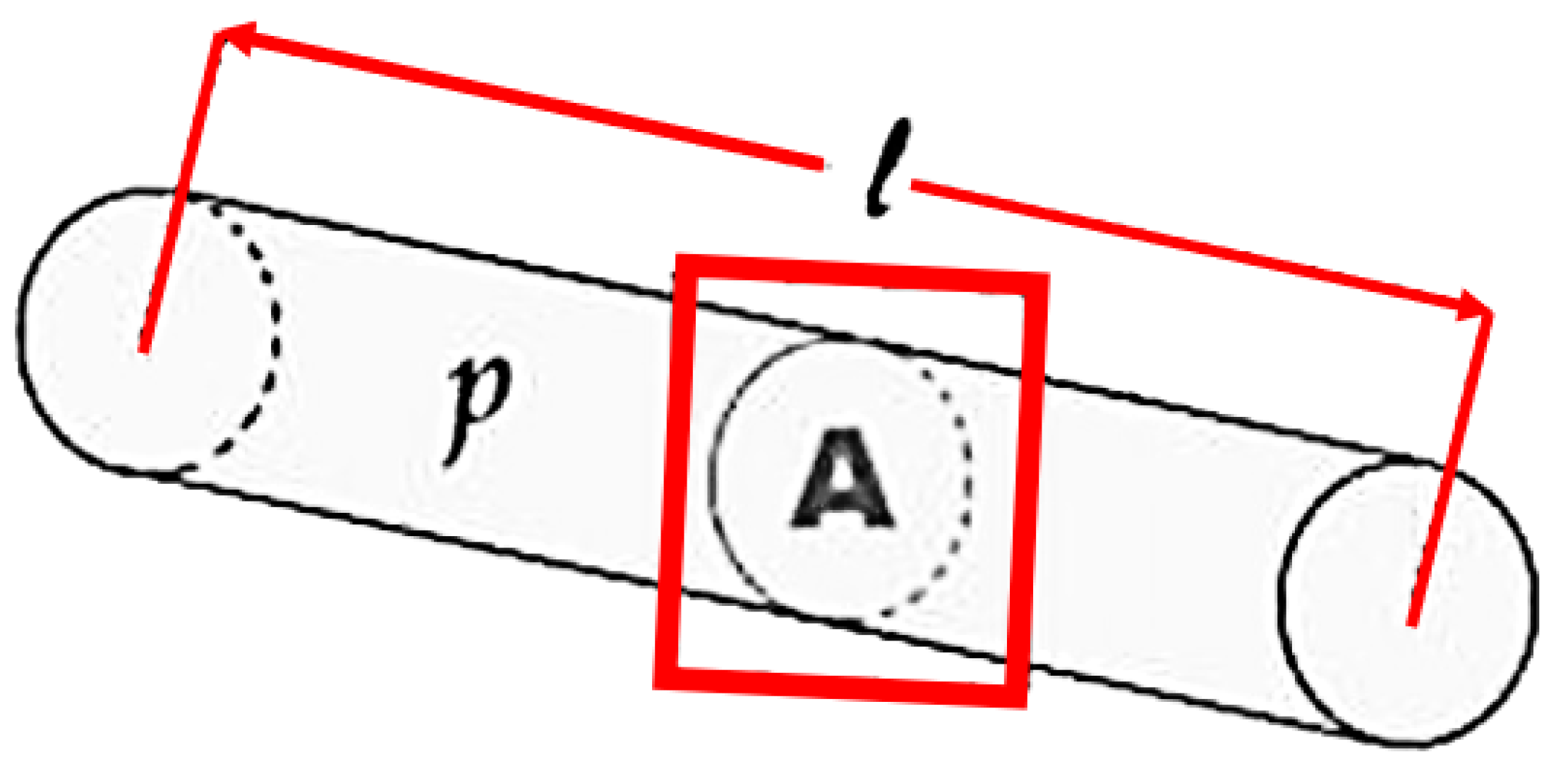
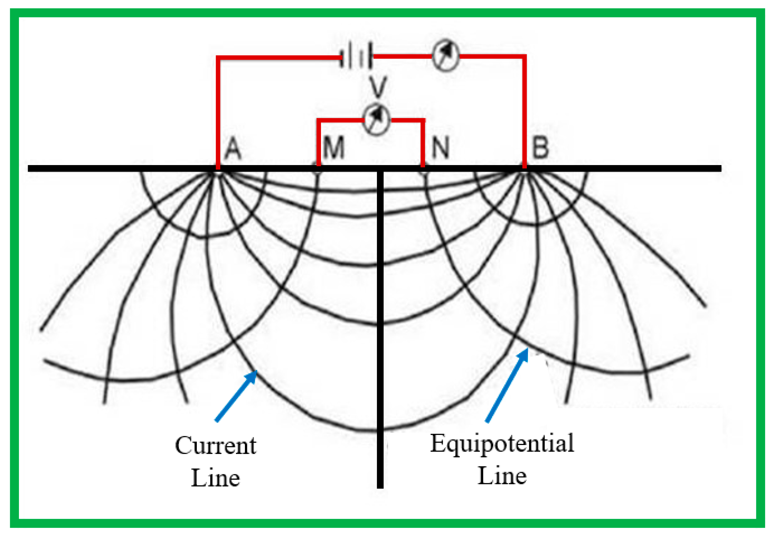
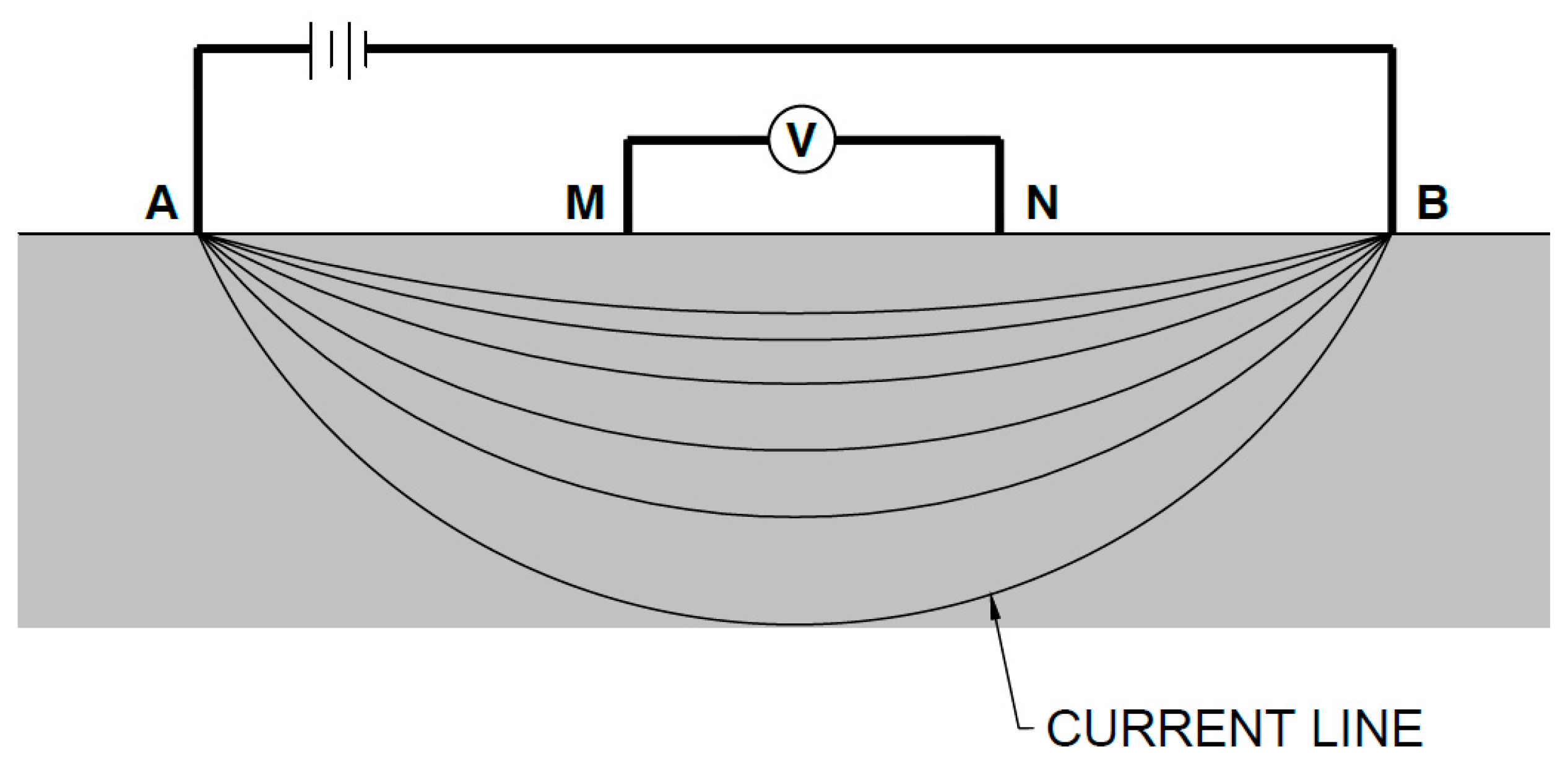
2.1. Basic
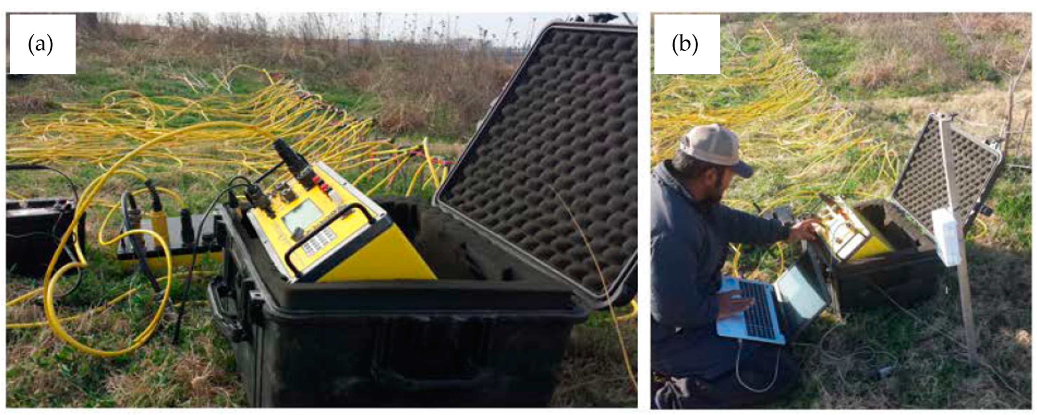
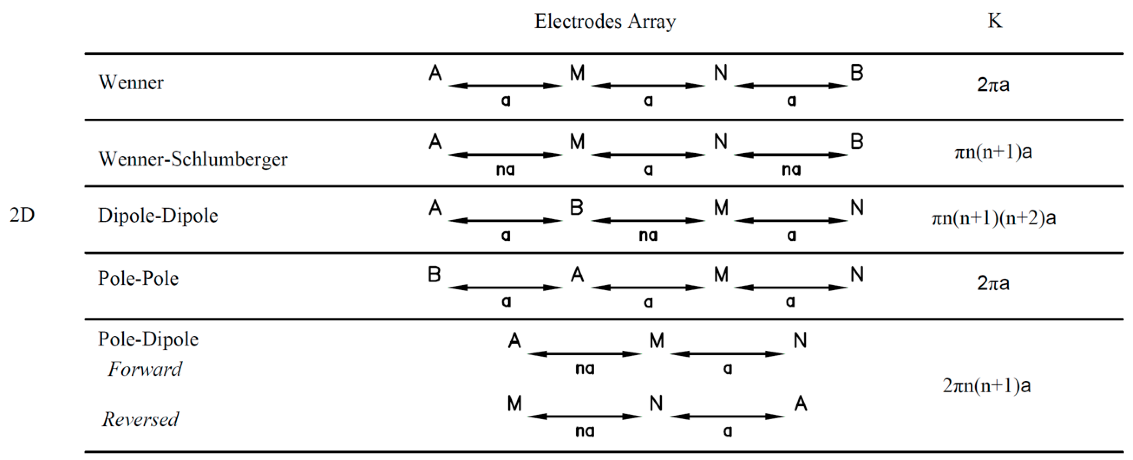
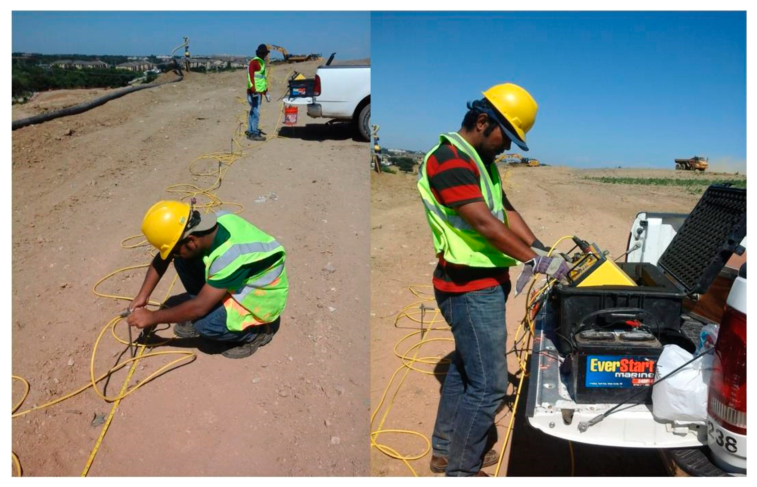
2.2. Data Acquisition
2.3. Data Interpretation
3. Case Studies
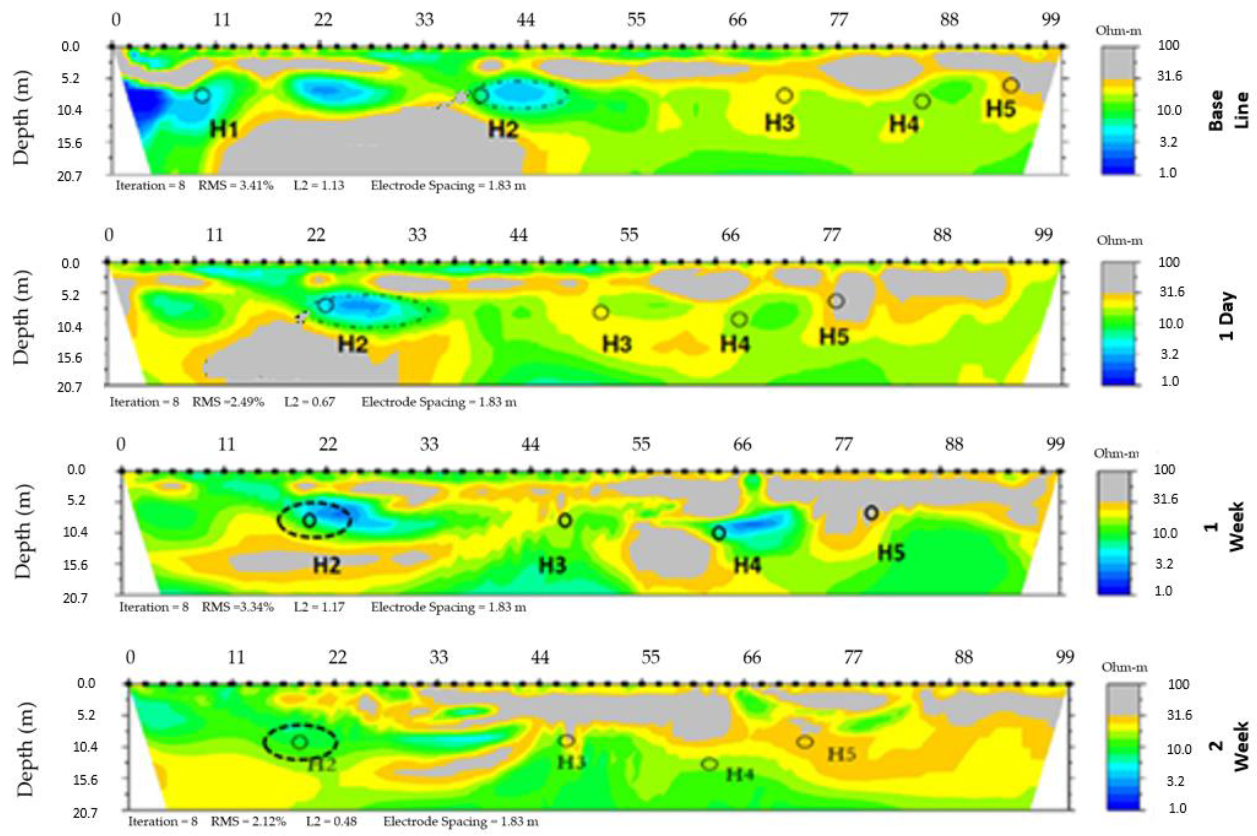
3.1. Case Study 1: Determination of Leachate Recirculation Frequency in Denton Landfill
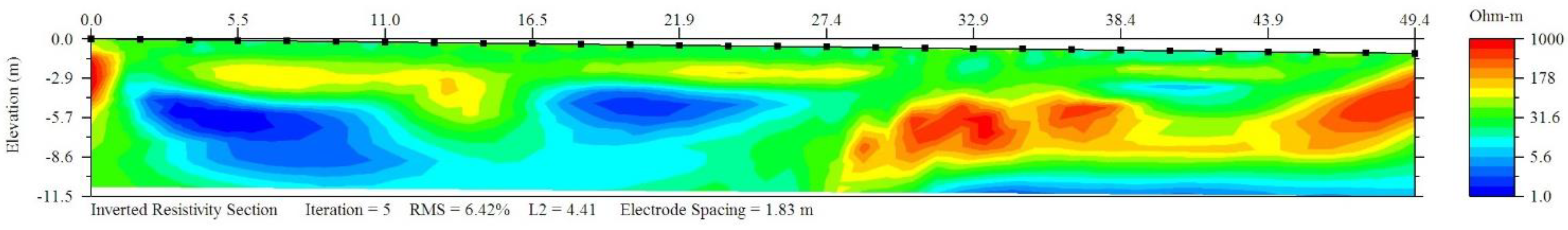
3.1.1. Description
3.1.2. Result
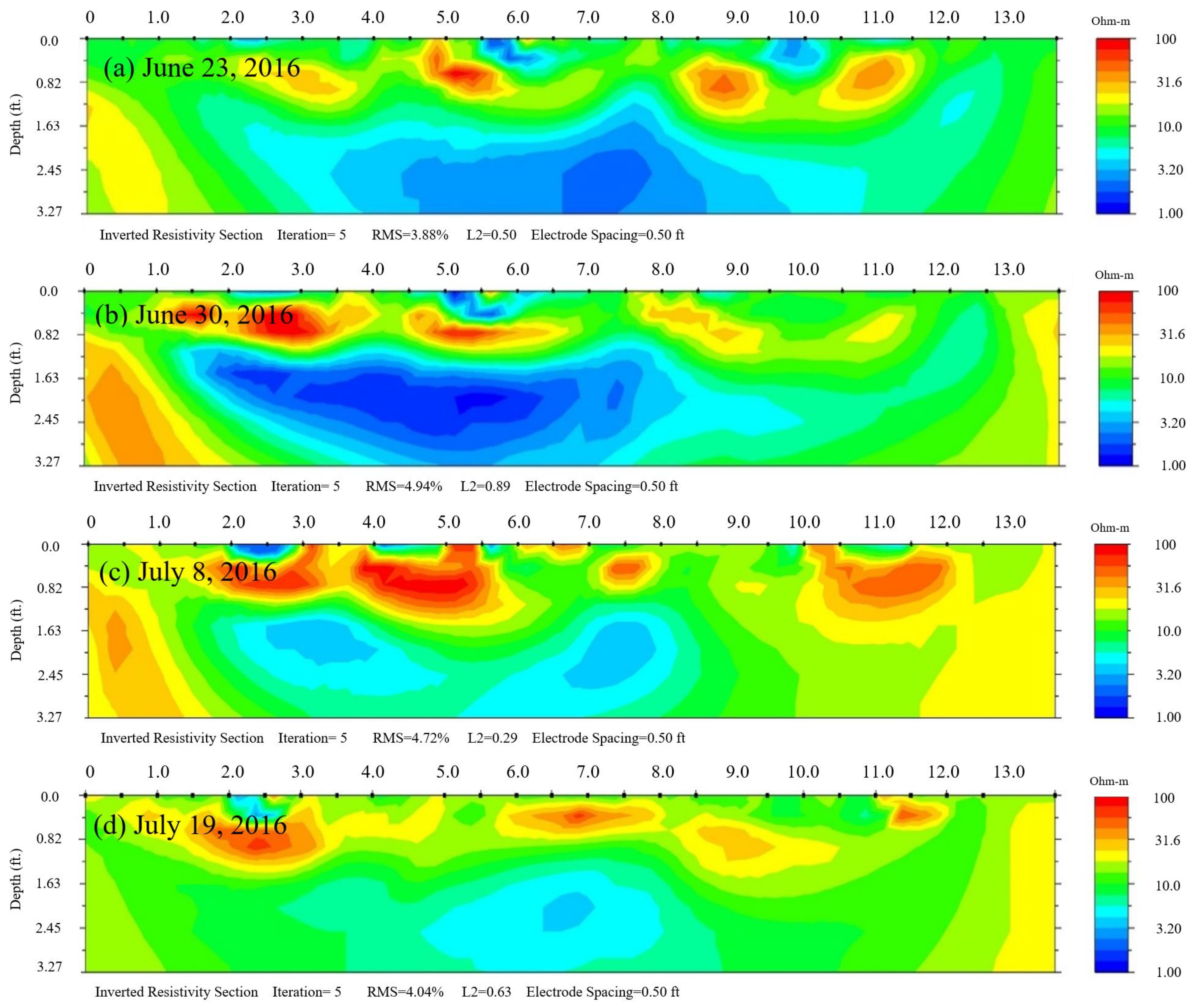
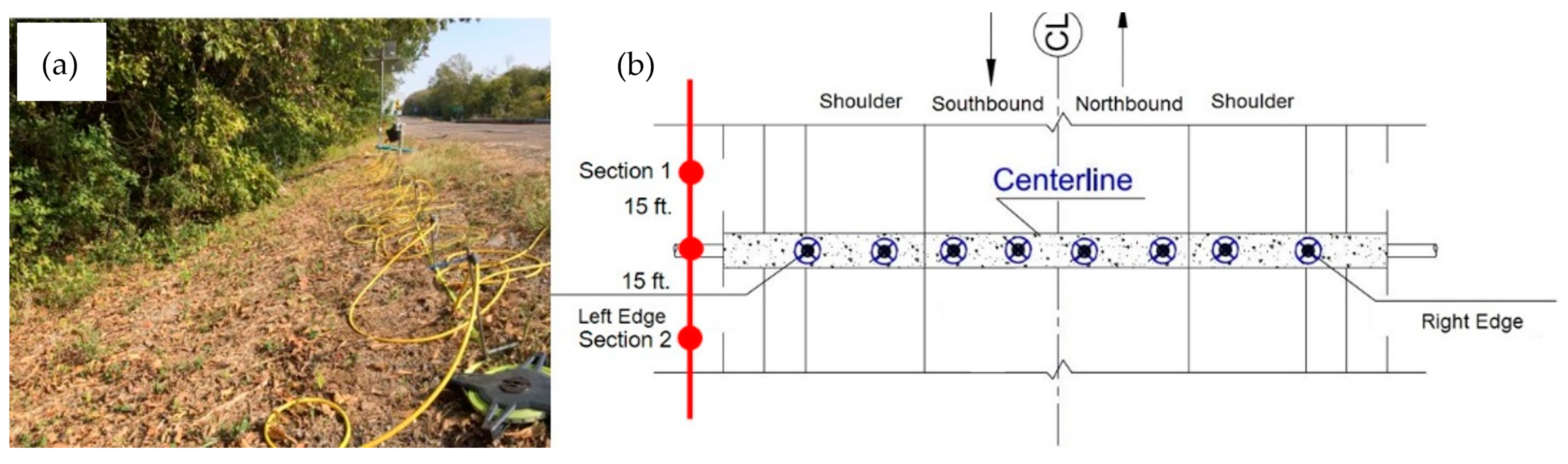
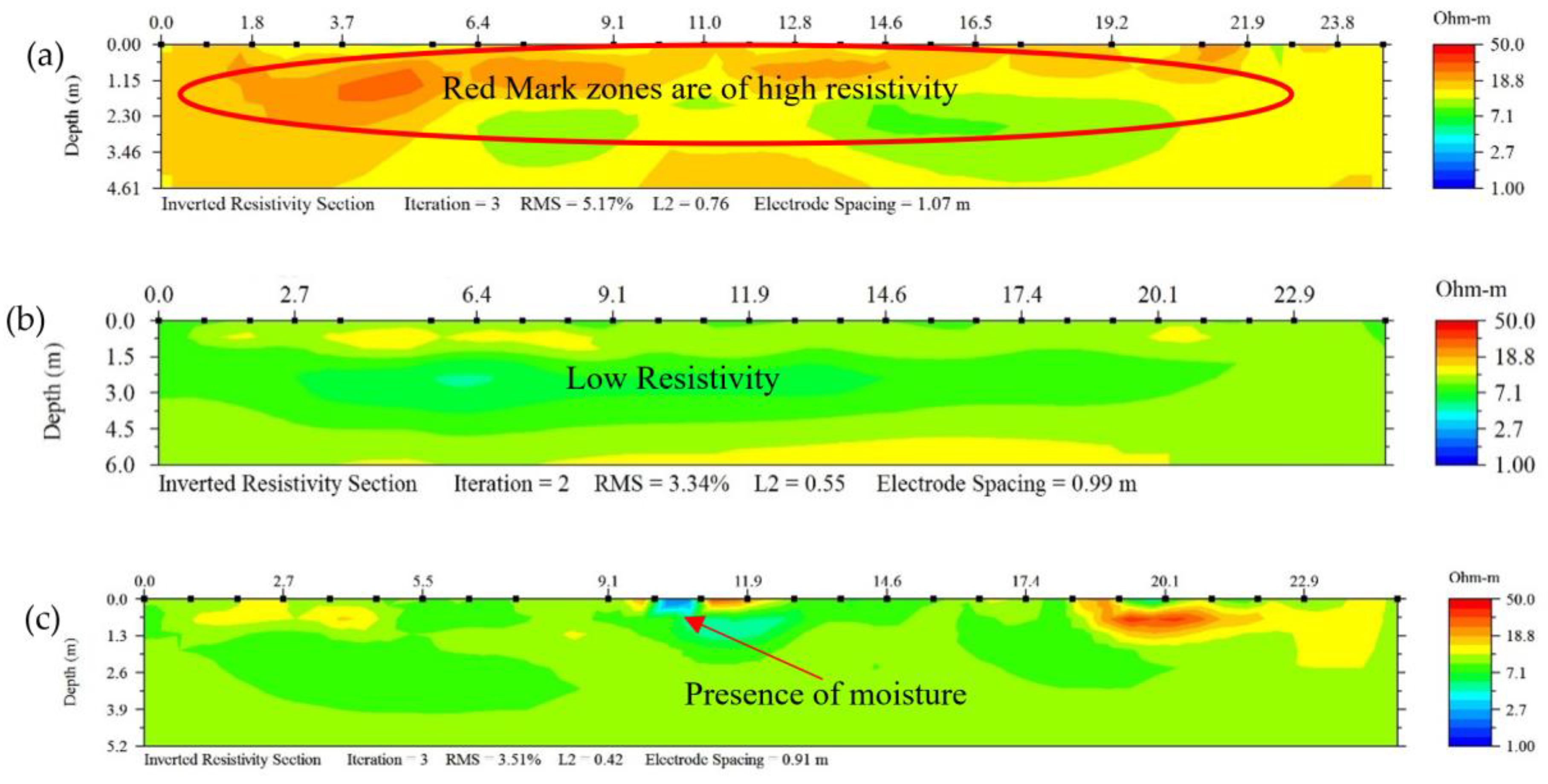
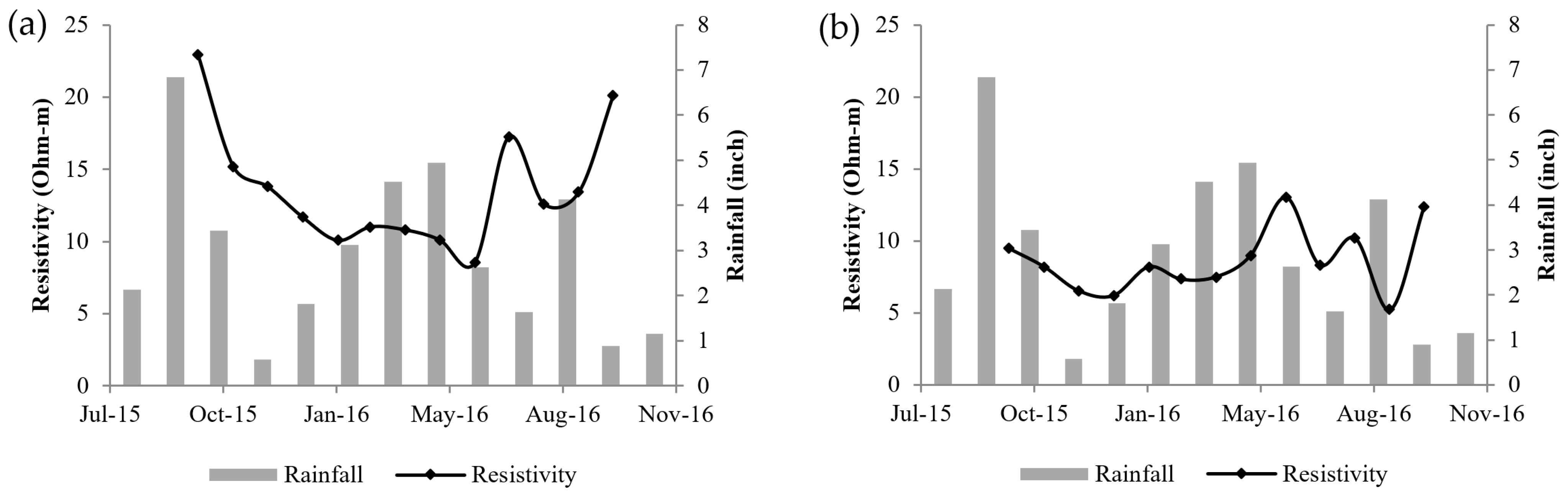
3.2. Case Study 2: Use of Resistivity Tomography in Pavement Moisture Distribution
3.2.1. Description
3.2.2. Result
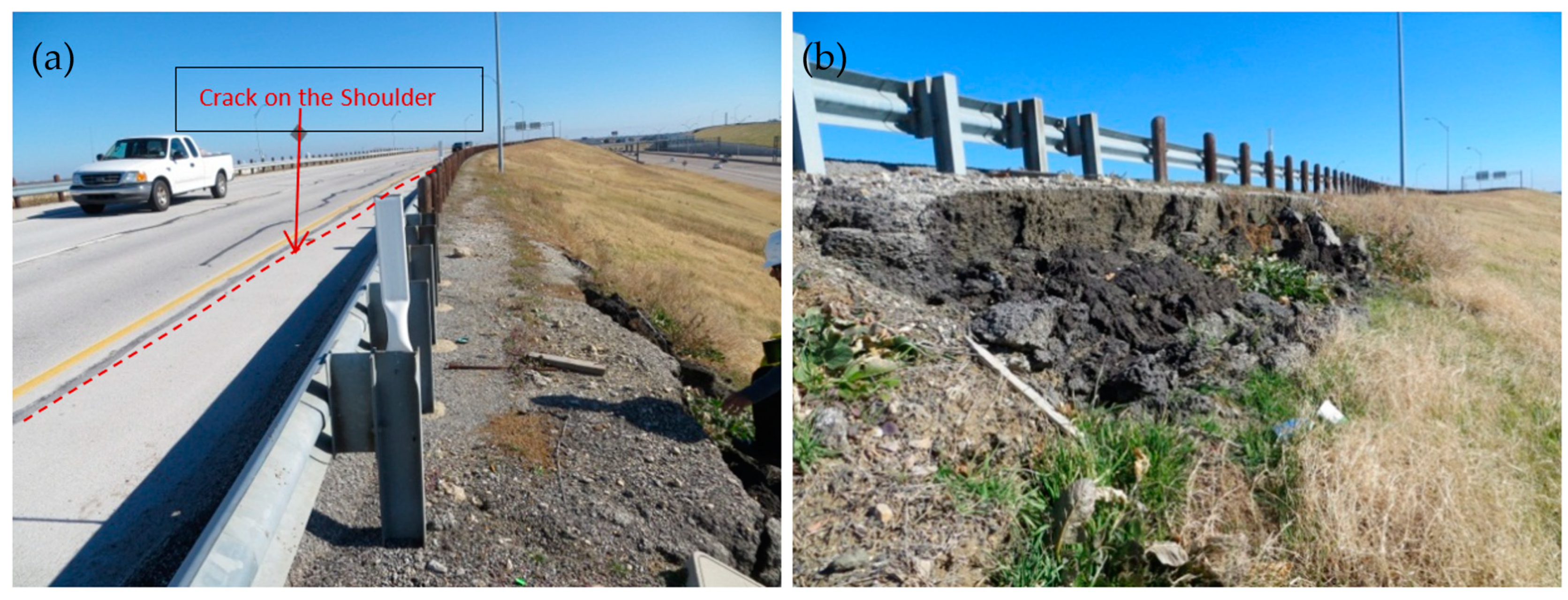
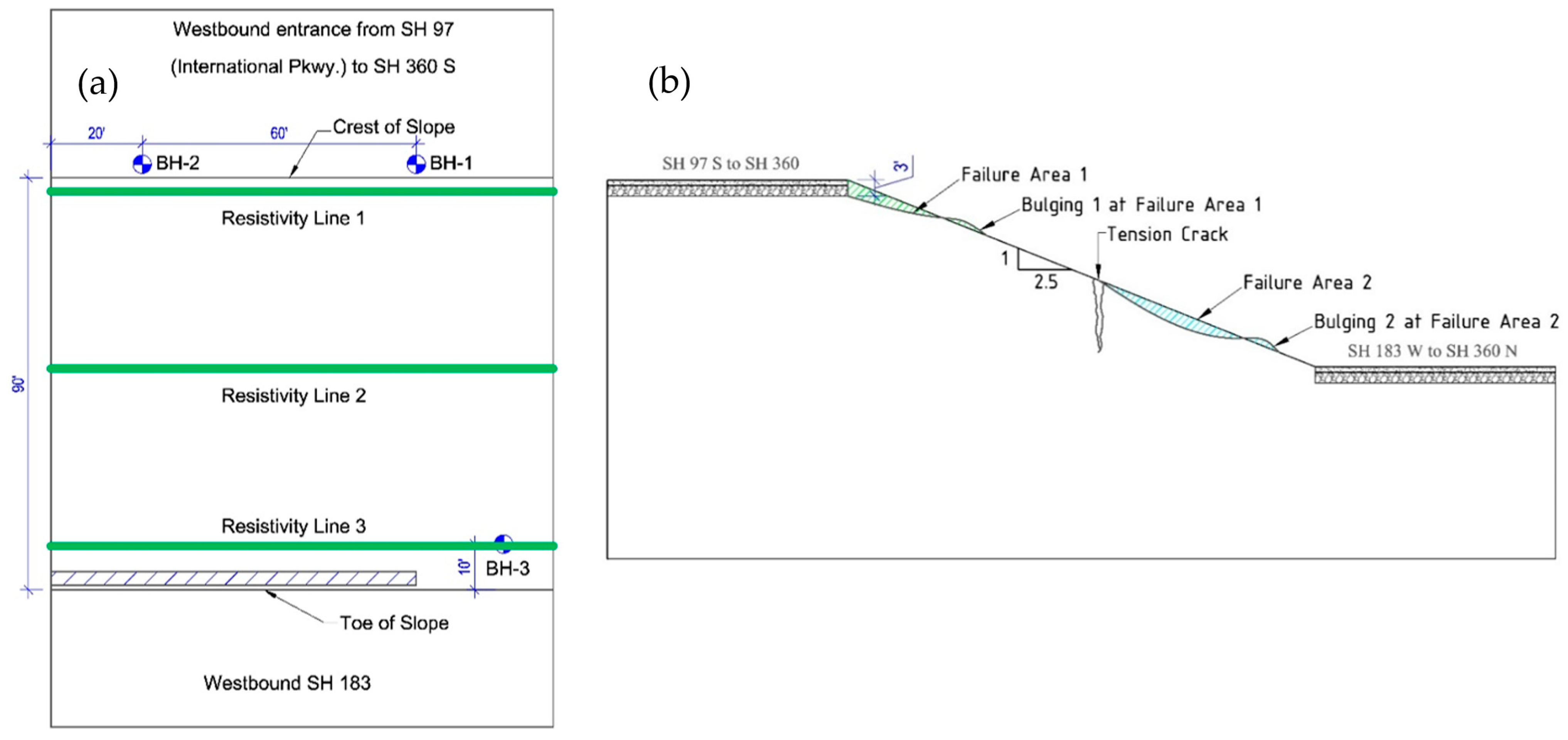
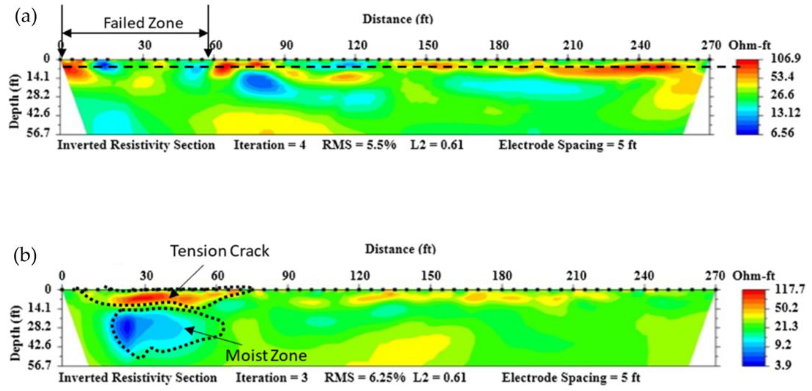
3.3. Case Study 3: Resistivity Tomography in Slope Failure Investigation
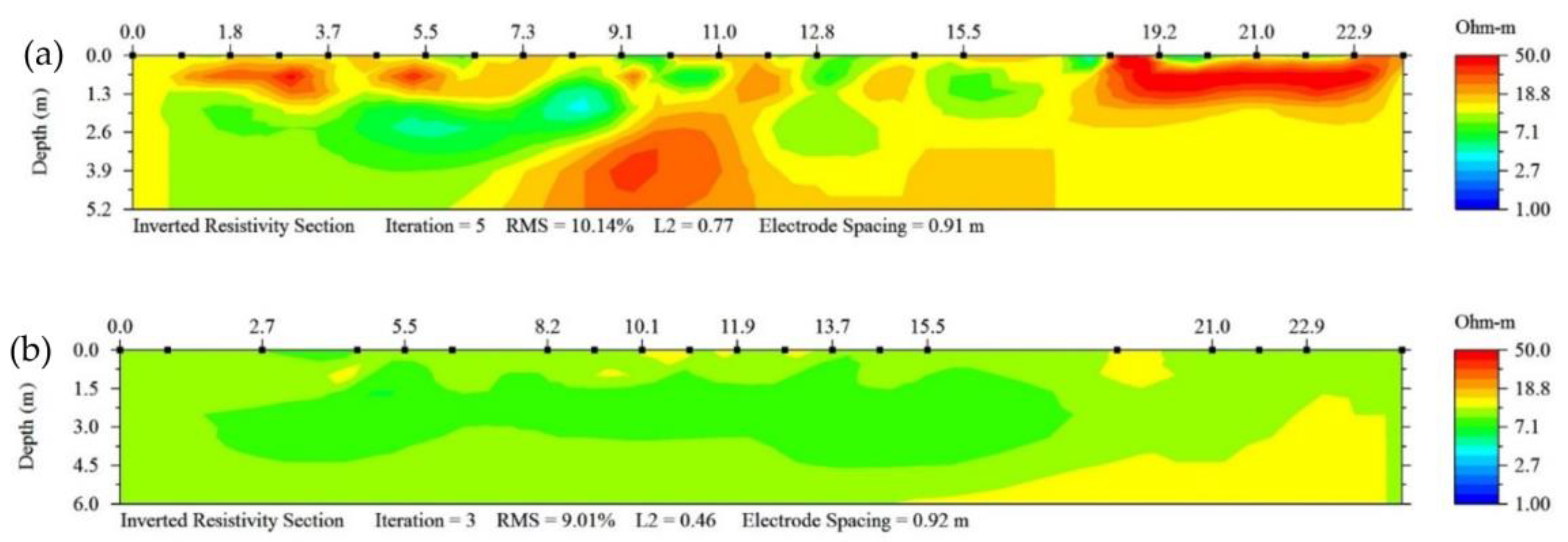
3.3.1. Description
3.3.2. Result
3.4. Case Study 4: ERT in Landfill ET Cover to Determine Moisture Variation
3.4.1. Description
3.4.2. Result
4. Discussion
- For leachate recirculation in landfills for ELR operation, it was perceived that moisture in the waste mass reaches the equilibrium condition after approximately 14 days. The ERT method adequately captured the moisture distribution which assisted in reaching this conclusion.
- The perched water zone was satisfactorily located using ERT during a slope failure investigation along a state highway. The failed portion of the slope was repaired accordingly after the extent of failure depth and moisture-prone zone were detected based on the ERT investigation.
- Seasonal moisture variation in the pavement was successfully captured using the ERT method. From two years of field investigation, May–October was found to be the dry period, whereas November–April was recorded as the wet season.
- Moisture–suction relationship of the ET cover soil was recorded via ERT testing. The top few inches of the cover soil (root zone) exhibited a significant change in resistivity values in different seasons of the year, indicating the efficiency of ERT in evaluating the seasonal moisture variation of ET cover soil. These findings were later correlated with the percolation of the ET cover.
Author Contributions
Funding
Data Availability Statement
Conflicts of Interest
References
- Tabbagh, A.; Dabas, M.; Hesse, A.; Panissod, C. Soil resistivity: A non-invasive tool to map soil structure horizonation. Geoderma 2000, 97, 393–404. [Google Scholar] [CrossRef]
- Samouëlian, A.; Cousin, I.; Tabbagh, A.; Bruand, A.; Richard, G. Electrical Resistivity Survey in Soil Science: A Review. Soil Tillage Res. 2005, 83, 173–193. [Google Scholar] [CrossRef]
- Aizebeokhai, A.P. 2D and 3D geoelectrical resistivity imaging: Theory and field design. Sci. Res. Essays 2010, 5, 3592–3605. [Google Scholar]
- Jabrane, O.; Martínez-Pagán, P.; Martínez-Segura, M.A.; Alcalá, F.J.; El Azzab, D.; Vásconez-Maza, M.D.; Charroud, M. Integration of Electrical Resistivity Tomography and Seismic Refraction Tomography to Investigate Subsiding Sinkholes in Karst Areas. Water 2023, 15, 2192. [Google Scholar] [CrossRef]
- Martínez-Pagán, P.; Gómez-Ortiz, D.; Martín-Crespo, T.; Manteca, J.; Rosique, M. The electrical resistivity tomography method in the detection of shallow mining cavities. A case study on the Victoria Cave, Cartagena (SE Spain). Eng. Geol. 2013, 156, 1–10. [Google Scholar] [CrossRef]
- Ghorbani, A.; Revil, A.; Bonelli, S.; Barde-Cabusson, S.; Girolami, L.; Nicoleau, F.; Vaudelet, P. Occurrence of sand boils landside of a river dike during flooding: A geophysical perspective. Eng. Geol. 2024, 329, 107403. [Google Scholar] [CrossRef]
- Franco, L.M.; La Terra, E.F.; Panetto, L.P.; Fontes, S.L. Integrated application of geophysical methods in Earth dam monitoring. Bull. Eng. Geol. Environ. 2024, 83, 62. [Google Scholar] [CrossRef]
- Hinojosa, H.R.; Kirmizakis, P.; Soupios, P. Historic Underground Silver Mine Workings Detection Using 2D Electrical Resistivity Imaging (Durango, Mexico). Minerals 2022, 12, 491. [Google Scholar] [CrossRef]
- Bharti, A.K.; Singh, K.K.K.; Ghosh, C.N.; Mishra, K. Detection of subsurface cavity due to old mine workings using electrical resistivity tomography: A case study. J. Earth Syst. Sci. 2022, 131, 39. [Google Scholar] [CrossRef]
- Arjwech, R.; Ruansorn, T.; Schulmeister, M.; Everett, M.E.; Thitimakorn, T.; Pondthai, P.; Somchat, K. Protection of electricity transmission infrastructure from sinkhole hazard based on electrical resistivity tomography. Eng. Geol. 2021, 293, 106318. [Google Scholar] [CrossRef]
- Suzuki, K.; Toda, S.; Kusunoki, K.; Fujimitsu, Y.; Mogi, T.; Jomori, A. Case studies of electrical and electromagnetic methods applied to mapping active faults beneath the thick quaternary. Dev. Geotech. Eng. 2000, 84, 29–45. [Google Scholar]
- Beauvais, A.; Ritz, M.; Parisot, J.-C.; Bantsimba, C.; Dukhan, M. Combined ERT and GPR methods for investigating two-stepped lateritic weathering systems. Geoderma 2004, 119, 121–132. [Google Scholar] [CrossRef]
- Maillet, G.M.; Rizzo, E.; Revil, A.; Vella, C. High resolution electrical resistivity tomography (ERT) in a transition zone environment: Application for detailed internal architecture and infilling processes study of a rhône river paleo-channel. Mar. Geophys. Res. 2005, 26, 317–328. [Google Scholar] [CrossRef]
- Hauck, C. Frozen ground monitoring using DC resistivity tomography. Geophys. Res. Lett. 2002, 29, 12-1–12-4. [Google Scholar] [CrossRef]
- Zhou, Q.Y.; Shimada, J.; Sato, A. Three-dimensional spatial and temporal monitoring of soil water content using electrical resistivity tomography. Water Resour. Res. 2001, 37, 273–285. [Google Scholar] [CrossRef]
- Hossain, M.S.; Maganti, D.; Hossain, J. Assessment of geo-hazard potential and site investigations using Resistivity Imaging. Int. J. Environ. Technol. Manag. 2010, 13, 116–129. [Google Scholar] [CrossRef]
- McCarter, W.J. The electrical resistivity characteristics of compacted clays. Geotechnique 1984, 34, 263–267. [Google Scholar] [CrossRef]
- Abu-Hassanein, Z.S.; Benson, C.H.; Blotz, L.R. Electrical resistivity of compacted clays. J. Geotech. Eng. 1996, 122, 397–406. [Google Scholar] [CrossRef]
- Ekwue, E.; Bartholomew, J. Electrical conductivity of some soils in Trinidad as affected by density, water and peat content. Biosyst. Eng. 2011, 108, 95–103. [Google Scholar] [CrossRef]
- Kalinski, R.; Kelly, W. Estimating water content of soils from electrical resistivity. Geotech. Test. J. 1993, 16, 323–329. [Google Scholar] [CrossRef]
- Giao, P.; Chung, S.; Kim, D.; Tanaka, H. Electric imaging and laboratory resistivity testing for geotechnical investigation of Pusan clay deposits. J. Appl. Geophys. 2003, 52, 157–175. [Google Scholar] [CrossRef]
- Power, C.; Gerhard, J.I.; Karaoulis, M.; Tsourlos, P.; Giannopoulos, A. Evaluating four-dimensional time-lapse electrical resistivity tomography for monitoring DNAPL source zone remediation. J. Contam. Hydrol. 2014, 162–163, 27–46. [Google Scholar] [CrossRef]
- Ali, M.A.H.; Sun, S.; Qian, W.; Dodo, B.A. Electrical resistivity imaging for detection of hydrogeological active zones in karst areas to identify the site of mining waste disposal. Environ. Sci. Pollut. Res. 2020, 27, 22486–22498. [Google Scholar] [CrossRef] [PubMed]
- Ahmed, A.; Hossain, M.S.; Khan, M.S.; Greenwood, K.; Shishani, A. Moisture Variation in Expansive Subgrade through Field Instrumentation and Geophysical Testing. In Proceedings of the International Congress and Exhibition “Sustainable Civil Infrastructures: Innovative Infrastructure Geotechnology”, Sharm El Sheikh, Egypt, 15–19 July 2017; Springer: Cham, Switzerland, 2017; pp. 45–58. [Google Scholar]
- Alam, M.Z.; Hossain, M.S.; Samir, S. Performance Evaluation of a Bioreactor Landfill Operation. In Proceedings of the Geotechnical Frontiers 2017, Orlando, FL, USA, 12–15 March 2017. [Google Scholar]
- Ozcep, F.; Tezel, O.; Asci, M. Correlation between electrical resistivity and soil-water content: Istanbul and Golcuk. Int. J. Phys. Sci. 2009, 4, 362–365. [Google Scholar]
- Hossain, M.S.; Khan, M.S.; Hossain, J.; Kibria, G.; Taufiq, T. Evaluation of unknown foundation depth using different ndt methods. J. Perform. Constr. Facil. 2013, 27, 209–214. [Google Scholar] [CrossRef]
- U.S. Environmental Protection Agency (EPA). Fact Sheet on Evapotranspiration Cover Systems for Waste Containment; Office of Solid Waste and Emergency Response: Washington, DC, USA, 2011.
- Binley, A. Tools and techniques: DC electrical methods. In Treatise on Geophysics, 2nd ed.; Schubert, G., Ed.; Elsevier: Amsterdam, The Netherlands, 2015; Volume 11, pp. 233–259. [Google Scholar]
- Lerner, L.S. Physics for Scientists and Engineers; Jones & Bartlett Learning: Burlington, MA, USA, 1996; Volume 1. [Google Scholar]
- Millikan, R.A.; Bishop, E.S. Elements of Electricity: A Practical Discussion of the Fundamental Laws and Phenomena of Electricity and Their Practical Applications in the Business and Industrial World; American Technical Society: Orland Park, IL, USA, 1917. [Google Scholar]
- Manzur, S. Hydraulic Performance Evaluation of Different Recirculation Systems for ELR/Bioreactor Landfills. Ph.D. Thesis, The University of Texas at Arlington, Arlington, TX, USA, 2013. [Google Scholar]
- Advanced Geosciences, Inc. Instruction Manual for Earth Imager 2D Version 1.7.4: Resistivity and IP Inversion Software; Advanced Geosciences, Inc.: Austin, TX, USA, 2004. [Google Scholar]
- Manzur, S.R.; Hossain, S.; Kemler, V.; Khan, M.S. Monitoring extent of moisture variations due to leachate recirculation in an ELR/bioreactor landfill using resistivity imaging. Waste Manag. 2016, 55, 38–48. [Google Scholar] [CrossRef] [PubMed]
- Shihada, H.; Hossain, M.S.; Kemler, V.; Dugger, D. Estimating moisture content of landfilled municipal solid waste without drilling: Innovative approach. J. Hazard. Toxic Radioact. Waste 2013, 17, 317–330. [Google Scholar] [CrossRef]
- Buettner, M.; Daily, W.; Ramirez, A. Electronic (sic) Resistance Tomography Imaging of Spatial Moisture Distribution, Moisture Distribution, and Movement in Pavements (Electrical Resistance Tomography for Monitoring the Infiltration of Water into a Pavement Section); FHWA/CA/OR-98-05; California Department of Transportation: Sacramento, CA, USA, 1997. [Google Scholar]
- Clarke, C.R. Monitoring Long-Term Subgrade Moisture Changes with Electrical Resistivity Tomography. In Proceedings of the Fourth International Conference on Unsaturated Soils, Carefree, AZ, USA, 2–6 April 2006; American Society of Civil Engineers: Carefree, AZ, USA, 2006; pp. 258–268. [Google Scholar]
- Hossain, S.; Ahmed, A.; Khan, M.S.; Aramoon, A.; Thian, B. Expansive Subgrade Behavior on a State Highway in North Texas. In Proceedings of the Geotechnical and Structural Engineering Congress, Phoenix, AZ, USA, 14–17 February 2016; American Society of Civil Engineers: Phoenix, AZ, USA, 2016; pp. 1186–1197. [Google Scholar]
- George, A.M.; Chakraborty, S.; Das, J.T.; Pedarla, A.; Puppala, A.J. Understanding shallow slope failures on expansive soil embankments in north texas using unsaturated soil property framework. In Proceedings of the Second Pan-American Conference on Unsaturated Soils, Dallas, TX, USA, 12–15 November 2017; pp. 206–216. [Google Scholar]
- Ahmed, A.; Khan, S.; Hossain, S.; Sadigov, T.; Bhandari, P. Safety prediction model for reinforced highway slope using a machine learning method. Transp. Res. Rec. J. Transp. Res. Board 2020, 2674, 761–773. [Google Scholar] [CrossRef]
- Khan, M.S.; Hossain, S.; Ahmed, A.; Faysal, M. Investigation of a shallow slope failure on expansive clay in Texas. Eng. Geol. 2017, 219, 118–129. [Google Scholar] [CrossRef]
- Benson, C.H.; Albright, W.H.; Roesler, A.C.; Abichou, T. Evaluation of final cover performance: Field data from the alternative cover assessment program (ACAP). Proc. Waste Manag. 2002, 2, 1–15. [Google Scholar]
- Khire, M.; Benson, C.; Bosscher, P. Water Balance Modeling of Earthen Landfill Covers. J. Geotech. Geoenviron. Eng. 1997, 123, 744–754. [Google Scholar] [CrossRef]
- Ogorzalek, A.S.; Bohnhoff, G.L.; Shackelford, C.D.; Benson, C.H.; Apiwantragoon, P. Comparison of field data and water-balance predictions for a capillary barrier cover. J. Geotech. Geoenvironmental Eng. 2008, 134, 470–486. [Google Scholar] [CrossRef]
- Bohnhoff, G.L.; Ogorzalek, A.S.; Benson, C.H.; Shackelford, C.D.; Apiwantragoon, P. Field Data and Water-Balance Predictions for a Monolithic Cover in a Semiarid Climate. J. Geotech. Geoenvironmental Eng. 2009, 135, 333–348. [Google Scholar] [CrossRef]
- Alam, M.J.B.; Hossain, M.S.; Sarkar, L.; Rahman, N. Evaluation of Field Scale Unsaturated Soil Behavior of Landfill Cover through Geophysical Testing and Instrumentation. In Proceedings of the Geo-Congress 2019: Eighth International Conference on Case Histories in Geotechnical Engineering, Philadelphia, PA, USA, 24–27 March 2019; pp. 1–11. [Google Scholar]
- Bin Alam, J.; Sarker, L.; Sapkota, A.; Ahmed, R.; Hossain, S. Evaluation of Soil Water Storage (SWS) of Evapotranspiration Cover through Geophysical Investigation. In Proceedings of the Geo-Congress 2020, Minneapolis, MN, USA, 25–28 February 2020; pp. 444–453. [Google Scholar]


| Base Line | 1 Day | 1 Week | 2 Week | |
|---|---|---|---|---|
| Pipe | MC (%) | MC (%) | MC (%) | MC (%) |
| H2 | 36.31 | 63.35 | 49.77 | 36.78 |
| H16 | 31.48 | 59.38 | 47.03 | 32.68 |
| H18 | 33.09 | 63.35 | 45.16 | 31.02 |
Disclaimer/Publisher’s Note: The statements, opinions and data contained in all publications are solely those of the individual author(s) and contributor(s) and not of MDPI and/or the editor(s). MDPI and/or the editor(s) disclaim responsibility for any injury to people or property resulting from any ideas, methods, instructions or products referred to in the content. |
© 2024 by the authors. Licensee MDPI, Basel, Switzerland. This article is an open access article distributed under the terms and conditions of the Creative Commons Attribution (CC BY) license (https://creativecommons.org/licenses/by/4.0/).
Share and Cite
Alam, M.J.B.; Ahmed, A.; Alam, M.Z. Application of Electrical Resistivity Tomography in Geotechnical and Geoenvironmental Engineering Aspect. Geotechnics 2024, 4, 399-414. https://doi.org/10.3390/geotechnics4020022
Alam MJB, Ahmed A, Alam MZ. Application of Electrical Resistivity Tomography in Geotechnical and Geoenvironmental Engineering Aspect. Geotechnics. 2024; 4(2):399-414. https://doi.org/10.3390/geotechnics4020022
Chicago/Turabian StyleAlam, Md Jobair Bin, Asif Ahmed, and Md Zahangir Alam. 2024. "Application of Electrical Resistivity Tomography in Geotechnical and Geoenvironmental Engineering Aspect" Geotechnics 4, no. 2: 399-414. https://doi.org/10.3390/geotechnics4020022
APA StyleAlam, M. J. B., Ahmed, A., & Alam, M. Z. (2024). Application of Electrical Resistivity Tomography in Geotechnical and Geoenvironmental Engineering Aspect. Geotechnics, 4(2), 399-414. https://doi.org/10.3390/geotechnics4020022