Abstract
In precedent years mostly, though rarely nowadays, shear deformable structures were constructed across the globe. Also, the soil is deformed as a shear cantilever, which means that the shear forces and stresses are more prominent than the respective normal forces and stresses; thus, the dynamic soil–structure interaction of shear deformable bodies is an important aspect to be researched. In this article, the dynamic soil–structure interaction of shear deformable structures is investigated through nonlinear finite element modelling. The goal of this work is to enlighten the qualitative response of both soil and structures, as well as the differences between the sole structure and the soil–structure system. The Athens 1999 earthquake accelerogram is used, which is considered as a palm load (which means a load that is not periodic like the Ricker wavelets), in order to enlighten the importance of the investigation of palm loading. It is demonstrated that the total displacements of the soil–structure system are larger than the case of the sole structure, as expected when taking into account the dynamic soil–structure interaction. However, the residual displacements of the top are larger when a moderate soil thickness is assumed. Moreover, the output acceleration functions over time, comparing the same buildings as the sole building and as the soil-building system, have the same time function, but they are amplified with a constant value. As a consequence, the critical time of the maximum energy flux that is transmitted to the building is not dependent on the dynamic soil–structure interaction.
1. Introduction
The soil–structure interaction (SSI) plays an important role in the computational mechanics discipline and influences the structural and geotechnical design of all infrastructure. In the past, numerous seminal scientific publications enlightened the attributes and properties of SSI from a qualitative perspective [,,,,,,,,,]. In all these, it has been depicted that the distribution of stresses and strains in buildings differ compared to the presumption that derelicts SSI. In some cases, the estimated displacements and equivalent forces are smaller with the SSI assumption, leading to a more economic design of the structure; subsequently, the SSI adoption is beneficial for engineers and society. In some other cases, however, the SSI assumption leads to detrimental results in relation to the sole structure analysis, leading to a more expensive design with greater values of building dimensions. Research publications that examine SSI from a quantitative perspective have been published in large numbers as a consequence of the evolution of computer science [,,,,,,,,]. In the aforementioned literature, large progress has been made from the definition of an exact constitutive relation for the estimation of the distribution of stresses and strains to the amalgamation of variability estimation and artificial intelligence in geotechnics. In the research conducted before, in the two qualitative and quantitative analyses of the SSI, from the buildings situated far from neighbouring other infrastructure to the adjacent buildings exposed to pounding or to deep-founded power plants, it was proven that the infrastructure response is mainly affected by the soil mass material properties while the bearing capacity and flexibility of the infrastructure vary from the case when the SSI is not taken into account [,,,,,]. In precedent scientific publications, an alleviated amount of them investigated the shear deformable structures, and a portion of them refer to the dynamic soil–structure interaction between subsequent soil and a shear vulnerable building.
The reproduction of the boundary conditions in infinity is important in the computational tackling of the SSI numerical problem. Methods that estimate the corresponding forces at the boundary that result in a smaller computational domain are proposed [,,]. In the aforementioned algorithms, the initially greater computational domain is subjected to a defined wave and, subsequently, in the smaller computational domain, the time function of the output displacement, velocity, and acceleration are estimated with the aid of Fourier functions. Consequently, the equivalent forces that are obtained from the aforementioned time output functions are subjected to the alleviated soil space, and the respective performance of the SSI system is estimated. Alternative methods that have been employed to tackle the assumptions at infinity are the the transmitting boundaries, the infinite elements, the infinite boundaries, and the energy-absorbing layers, as well as the boundaries’ dashpots that provide energy dissipation and the boundary integral equation [,,,,,,]. When the mapped infinite element method is used, the boundary conditions at infinity are satisfied through the adding of the aforementioned infinite elements. Subsequently, the energy of the wave exits the computational domain instead of reflecting back. In addition, the dimensions of the boundaries may be adopted as infinite to satisfy the dimensionality in the far field of the computational domain. As a consequence, the energy absorption and the avoidance of wave reflections that would result in standing waves are both satisfied. Moreover, transmitting boundaries are adopted to achieve a more succinct computing space to obtain the desired precision, with the directivity of the flux where it should be directed. In conclusion, dissipating dashpots such as the Lysmer boundaries of velocity or the energy-dissipating layers are adopted for the prediction of the corresponding behaviour in a fair distance from infrastructure and soil and, subsequently, predict the response of the SSI computational domain of the soil in the vicinity of the infrastructure. The last pair of algorithms indicated incorporate the fact that energy dissipation can be achieved with the aid of velocity-influenced equations and, consequently, the energy does not reflect to fixed computational borders or similar respective conditions such as the underlying rock and, as a result, the standing waves, which do not occur in real conditions, are evaded. As for the boundary integral equation, the classical Galerkin ideas are implemented initially in 2D systems and, subsequently, this framework was extended to 3D space systems. The Galerkin formulation was adopted in the boundary considering an elastic border at infinity, and then the boundary element method was adopted to satisfy the conditions applied in the far field from the computational domain in discussion.
In this article, a numerical investigation for the dynamic soil–structure interaction problem for shear deformable structures is portrayed. The term shear deformable or, alternatively, shear vulnerable structures, will denote the superstructures where the shear stresses and forces are more profound in contrast to the normal stresses and forces and, subsequently, they are more probable to have a shear or brittle failure than bending or ductile failure. There are several scientific publications that deal with these kinds of structures, as they represent older structures that can collapse to an earthquake. The literature review consists of computational publications [,,,,] and investigations on real-world structures made of masonry walls [,,,,], steel structures [,,,,], and reinforced concrete structures [,,,,]. In the literature focusing on real-world structures, an experimental investigation of wall behaviour under shear loading is widely examined, and the effect on SSI systems is also estimated through the modelling of real-world structures. The aim of this work is to enlighten the properties of the dynamic soil–structure interaction behaviour in shear deformable structures when they are subjected to a nonsinusoidal force, particularly palm excitation. Moreover, this work tends to highlight the speed-up of the high performance computational methods to the prediction of the SSI response to dynamic loading. Hexahedral finite elements are implemented, and the material stress–strain law is the Von Mises yield criterion with perfect plasticity as hardening law. The hexahedral finite elements are implemented for both soil and structure simulation in order to obtain a qualitative behaviour of the shear deformable structure, instead of using Euler Bernoulli beams that neglect the shear deformation. The number of floors which is the total superstructure height to the element height are, respectively, 1, 2, and 5. The dead weights and the subsequent total mass comes from the consistent mass matrix of the finite element formulation with density 25 . The numerical equation of the boundary seismic excitation in nonlinear analyses is solved. Three different buildings and three different soil thicknesses are adopted, and all combinations are analysed, as well as the case of the sole building. The Athens 1999 earthquake is subjected to the computational systems, which is considered to be a palm force. The time history analyses are performed, and the output time functions of the total displacements, total accelerations and residual displacements are portrayed with the corresponding peak values. Also, the computational cost in terms with a corresponding linear elastic analysis is given and a comparison is given. The results stipulate that the total displacements when soil–structure interaction considered are greater, while the relative displacements are smaller and subsequently the equivalent loads. Moreover, the plastic residual displacements of the top of the building are the largest when moderate soil thickness is assumed. In conclusion, in a moderate soil thickness of 20 m, a resonance occurs. That leads to the largest energy flux that is subjected to the structure, and to the largest plastic residual deformations.
2. Dynamic Soil–Structure Interaction Formulation and Implicit Integration Algorithm
In computational mechanics, the SSI problem is a numerical dynamic problem of two kinds of degrees of freedom: the free degrees of freedom, which are unknown and are the ones of the building and the soil far from the boundaries, and the support degrees of freedom, which refer to the soil boundary degrees of freedom. By referring to the dynamic equation of motion and restructuring the degrees of freedom to free and support-excitation degrees , the following is obtained:
where, for the initial structured matrices of mass , damping and stiffness are formulated through the finite element method and the Rayleigh damping assumption as usual, with the implementation of the shape functions and deformation matrix :
In nonlinear analysis, the internal forces in free and support degrees of freedom are coupled. Therefore, Equation (1) is as follows:
Subsequently, since the equivalent forces are a function of the imposed displacements, and the Newmark scheme is not a function the convergence, more steps for convergence to Newton–Raphson algorithm are required. Moreover, the excitation may be synchronous or asynchronous in all degrees of freedom of the boundary. In the first case, Equation (1) leads to an easier numerical system.
Solving Equation (1) or Equation (3) is possible through an explicit time integration scheme like the central difference method and an implicit time integration scheme like Newmark method. In Newmark method, the generalized dynamic equation with the internal and external forces, respectively, is the following:
By employing the equations given hereinafter for connecting the displacements, the velocities and accelerations between the time steps chosen are:
where and are coefficients that are chosen for tuning the stability and the accuracy of the numerical scheme. The most common values for these coefficients, which are also implemented in this article, are and , which is called the trapezoidal rule integration scheme. Subsequently, Equation (5) is inserted into Equation (4), and the following linear system is constructed:
The Newmark nonlinear algorithm is stated as follows: After the selection of the and coefficients, the variables are calculated through Equation (6e,f). Subsequently, the effective stiffness matrix and the effective load vector are calculated through Equation (6b,c). The linear system Equation (6a) is solved with the implementation of the tangent stiffness matrix , and the iterative displacements are determined. Afterwards, the iterative displacements are added to the incremental displacements of a previous iteration, and the incremental displacements are subsequently added to the total displacements in the previous time step. The total displacements calculated are used in order to estimate the internal forces . Then, the effective internal forces are calculated through Equation (6c) by substituting the with . Then, the effective external load is compared with the effective internal load . If the difference lies between a desired tolerance, then a convergence is achieved. If this occurs, the total displacements are determined and, subsequently, the accelerations firstly and the velocities afterwards are determined through Equation (6d). If no convergence is achieved, a new iteration is performed for the residual load force . In both cases, the effective stiffness matrix is updated at the time when the internal equivalent loads are updated. The material constitutive model for stress–strain law for the solution of Equation (1) to be defined, in this article, is the Von Mises yield criterion. In this work, no hardening is present; subsequently, the yield function is the following for a possible triad of principal stresses () and yield stress :
and the constitutive matrix of an integration Gauss point is zero if the value of the yield function is zero or else a yield occurs.
In this article, the Von Mises yield stress–strain law is adopted for the solution of the numerical problem discussed, as it has been proven that, for saturated soils, it can be qualitatively be appropriate for the estimation of the saturated soil response. In [,,], it has been demonstrated the fitting of the aforementioned yield criterion for a substantial estimation prior to a numerical computation with more accurate material constitutive modelling. Moreover, the selection of the Newmark method is implemented because the seismic excitation has a not very large change in the momentum, like a Dirac phenomenon, thus the implicit scheme is more efficient for the aforementioned analysis and, consequently, the integration of the momentum of the external load can be performed without important loss. In [,,], it is portrayed that these particular advantages of the method led to the selection for the solution of the problem in discussion.
3. Nonlinear Computational Dynamics and the Energy Dissipation Dashpot through the Lysmer Proposal
When nonlinear analysis is considered, the main computational difficulty comes from the large amount of degrees of freedom, as well as the material nonlinearity and complexity. When increased accuracy is desired, the effort increases even more. An alleviation of the computational cost for the same quantitative quality of results may be obtained by incorporating a equivalent system that estimates the equivalent forces far from the SSI system, and then reflects these forces to the SSI computational model. Hereinafter, the [] boundary dashpot theory of the model reduction methods is analysed, and a damping matrix for the implementation of the finite element analysis is proposed. Let the 1D wave propagation equation be:
Let us assume that:
It can be justified that
The last equation states that a dashpot may be assumed with value be its actual ratio. By calculating the virtual work, this can be implemented in finite element code. Subsequently, the following are obtained:
Denoting are the velocity of the longitudinal and shear waves, as well as the shape functions in global axes X, Y, Z. Moreover, are the density, the thickness in direction Y and Z, respectively. The integral in hexahedral element is given hereinafter, by denoting :
This version of the integral with the consistent operation of the estimation of the damping matrix is justified to result to more accurate estimations. Nevertheless, the lumped dashpots proposition can also be implemented sometimes. The procedure and efficiency of the aforementioned theory in this chapter is the following: by estimating the matrix given in Equation (12) and adding it in the damping matrix of the reduced domain skeleton, a numerical energy dissipation occurs. This results to avoidance of reflections of the travelling waves and subsequent creation of standing waves. Moreover, the computational gain is such that, since a reduced computational scheme which is obtained, the algebraic linear systems to be solved is solved without proportional loss to the accuracy of the output displacements computed. Subsequently, the implementation of the Lysmer dashpots by adding an additional damping matrix coefficient to the degrees of freedom laying in the border of the computational domain leads to a more fast to solve and with substantial accuracy. In this work, the consistent version of the energy dissipation is adopted for the investigation of its effect in the dynamic behaviour of a soil–structure interaction computational space for the demonstrations of the boundaries efficacy and importance in computational mechanics, with the constant re-estimate of the matrix with the updated shear and longitudinal velocities for comprising the nonlinear response of the border degrees of freedom.
4. Numerical Simulations of Shear Cantilevers of Free Field and Soil–Structure Interaction Systems in Dynamic Loading-Discussion
Hereinafter, the numerical analyses for the examination of the dynamic soil–structure interaction regarding shear vulnerable structures are portrayed. Initially, the geometric and material properties for each counterpart of the computational model are the following. For the soil domain, it is a rectangular parallelepiped with the dimension in the X axis to be the length, the dimension in Y axis to be the width and the dimension in Z axis to be the depth or soil thickness. It should be noted that , where is the length in the X axis and analogous conclusions occur for . The material properties of the soil domain is considered to be simulated as cohesive (e.g., slits or clays). This assumption was made in order to obtain the undrained strength of the soil which, in cohesive soils, is considerable, in contrast to cohesionless soils, which is negligible. For the geometric properties of the superstructure, a full rectangular parallelepiped, which means a full solid element, is also assumed as for obtaining the qualitative behaviour of the building. The top view of the structure is assumed as square of size 10 m. The total stiffness of the matrix is considered as the classical stiffness matrix of the finite element analysis to acquire for a floor height of 3 m. The material properties of the superstructure are considered as the appropriate ones for steel structures. This presumption was made in order to acquire for old industrial buildings that are a common type of shear deformable structure in all around the world. Free field models, which means soil domains without superstructure, containing a soil computational mesh constituted through hexahedral cubic finite elements of linear shape functions and size 10 m, acquiring the Von Mises yield envelope, are depicted in Figure 1, whilst the soil–structure interaction computational schemes, consisting of a soil mass counterpart that is constituted through hexahedral cubic finite elements of linear shape functions and size 10 m and a superstructure counterpart, constituted through the same type of full hexahedral elements (i.e., a full solid element), with the stress–strain constitutive model being the Von Mises envelope, are portrayed in Figure 2. In Table 1, the discretization meshes are given for all computational domains investigated, all of which are constituted through hexahedral cubic finite elements of linear shape functions and at a size of 10. The size of the computational domain has been selected in order to prevent wave reflections in the dynamic behaviour of the SSI computational domain. Furthermore, this presumption of discretization for the superstructure, namely the hexahedral cubic finite elements of linear shape functions, is a justifiable presumption made for shear vulnerable structures. In order to attain the desired behaviour of avoiding wave reflections, a parametric analysis has to be performed for the computational domain with and without energy absorption dashpots, such as the Lysmer dissipation boundaries and contrast the output time function of the monitored displacements and determine the size of the computational space of which the monitored displacements with and without energy dissipation dashpots concur. An analysis has been conducted for the effect of the reflections of the seismic waves with and without dashpots, and this has resulted in the computational mesh dimensions selected and depicted in Table 1, which are proven to have negligible influence to the response of the computational space. The material constitutive stress–strain law applied in both soil and structure, in all full parallelepiped solid elements, is the Von Mises material yield function with E = 1 GPa, and KPa comprising perfect plasticity as hardening law, as depicted in Table 2. Furthermore, the connection in the boundary between the soil and the structure is only through the elements common degrees of freedom kinematic condition of being the same without any other element or body to interconnect. This assumption is adopted due to having a qualitative estimation of the response of shear deformable structures subjected to dynamic load and investigating soil–structure interaction through the respective computational system. The Athens Earthquake of 1999 [,], shown in Figure 3, is adopted for the support excitation of degrees of freedom that corresponds in the right hand side of Equation (3), and the excitation is assumed to be synchronous; in other words, all of the support degrees of freedom are excited at the same time with the adopted accelerometer in the global X axis. In the global Y and Z axis the displacements, velocities and accelerations in the boundary surfaces are zero. As a result, the one dimensional excitation results to an alleviated amount of for accurately estimating the response of the sol domain and SSI computational space. For numerically justifying this attribute, a set of analyses with the free field soil domain and the SSI system were performed for a set of values , alongside different values for E = 1 GPa, 2 GPa, and 5 GPa, and the results are depicted in Table 3, which is situated hereinafter. It is demonstrated that the largest displacement and acceleration calculated in the top of the soil in the free field computational space and in the top of the structure in the SSI system are not diverging in percentage by more than 5%. This applies for all values of the ratio , as well as for E. A justification of the selection of the correct mesh through a convergence test and a validation of the analyses performed are found hereinafter, in Table 4 and Figure 4. It is demonstrated that the greatest percentage deviation in the mesh selected in the analyses in comparison with the finer meshes is no more than 5%. Adding to this, a validation analysis from the results obtained from the open source numerical code MSolve was made with ANSYS results as a comparison. A time-displacement curve was obtained for nonlinear dynamic analysis for a linearly increased dynamic load subjected to a cantilever simulated with hexahedral finite elements with linear shape function, such as the ones implemented in this work. The results coincide in an absolute way. Furthermore, the Rayleigh Damping constants are estimated by comprising the first and the second eigenfrequencies of an infinite shear cantilever, namely . In Figure 5, Figure 6, Figure 7, Figure 8, Figure 9, Figure 10, Figure 11, Figure 12, Figure 13, Figure 14, Figure 15, Figure 16, Figure 17, Figure 18, Figure 19, Figure 20, Figure 21 and Figure 22 and Table 5, which are positioned in the hereinafter, the total displacements and accelerations in the top of the structure with and without the soil–structure interaction, as well as with the peak values of the total displacements, the residual displacements that exist after the earthquake phenomenon, the accelerations and the ratio of the total to the residual displacements are depicted and discussed.
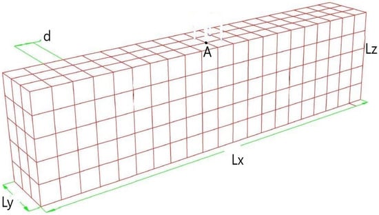
Figure 1.
Schematic representation of the free field computational scheme. The values , are found in Table 1, in the column “Meshes free field” and the value for d = 10 m. Point A stands for the upper middle point of the soil domain.
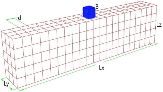
Figure 2.
Schematic representation of the SSI computational scheme. The values are found in Table 1, in the column “Meshes SSI system”, and the fourth value stands for the total height of the building coloured in blue, and is represented with blue line coloured full hexahedral solid finite elements, which are full parallelepipeds. Point B stands for the tip nodal displacement of the superstructure which is coloured in blue.

Table 1.
Mesh distribution in X-Y-Z dimension of the models. The dimensions are given and in the meshes in the SSI systems the last right value is the total height of the structure.
Table 2.
Material properties for the superstructure and the soil domain. H stands for the plastic hardening modulus.
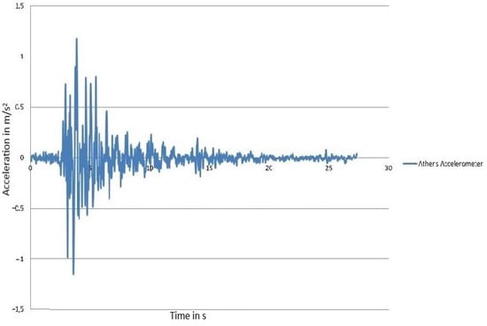
Figure 3.
The 1999 Athens Earthquake Accelerogram (Monastiraki).
Table 3.
Investigation of the influence of the in relation to the in the computational estimation of the output displacements and accelerations in the free field and SSI computational space by imposing 1 dimensional dynamic excitation.
Table 4.
Convergence analysis of the finite element mesh for the mesh selected for the analyses (cube of size 10 m) and other finer meshes.
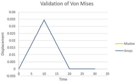
Figure 4.
Validation of the results obtained from the numerical open source computational mechanics code MSolve using ANSYS for comparison. A nonlinear dynamic analysis for a linearly increased dynamic load and Von Mises yield criterion has been implemented to a cantilever simulated with hexahedral finite elements with linear shape functions. The results coincide in an absolute way.
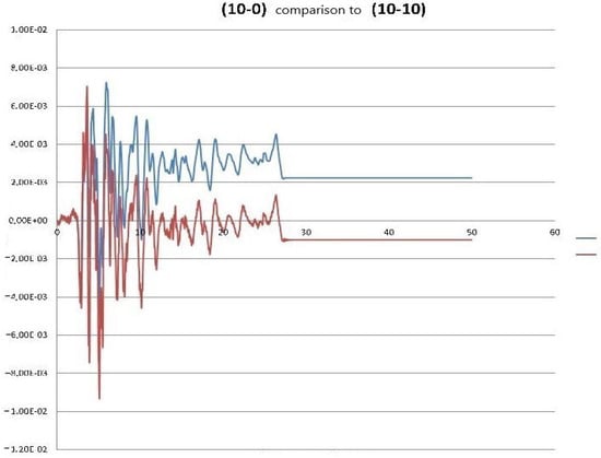
Figure 5.
Time functions of the total displacements for building top point in the X degree of freedom of height 10 m without soil (blue line) and for the same building with soil depth 10 m (red line). Horizontal axis: time in seconds, vertical axis: displacement in m.
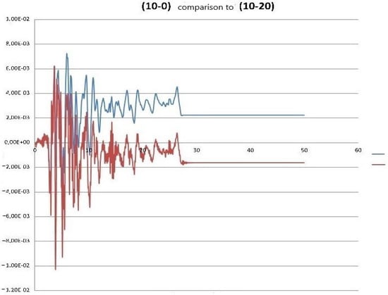
Figure 6.
Time functions of the total displacements for building top point in the X degree of freedom of height 10 m without soil (blue line) and for the same building with soil depth 20 m (red line). Horizontal axis: time in seconds, vertical axis: displacement in m.
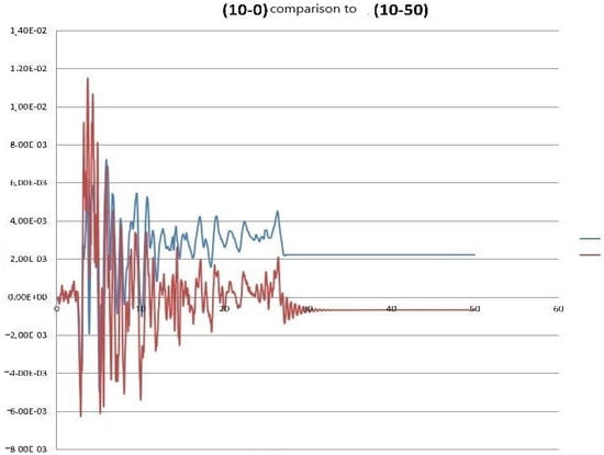
Figure 7.
Time functions of the total displacements for building top point in the X degree of freedom of height 10 m without soil (blue line) and for the same building with soil depth 50 m (red line). Horizontal axis: time in seconds, vertical axis: displacement in m.
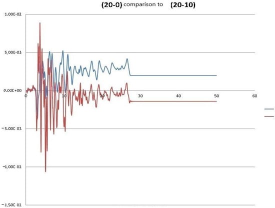
Figure 8.
Time functions of the total displacements for building top point in the X degree of freedom of height 20 m without soil (blue line) and for the same building with soil depth 10 m (red line). Horizontal axis: time in seconds, vertical axis: displacement in m.
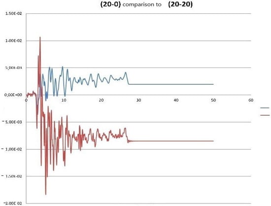
Figure 9.
Time functions of the total displacements for building top point in the X degree of freedom of height 20 m without soil (blue line) and for the same building with soil depth 20 m (red line). Horizontal axis: time in seconds, vertical axis: displacement in m.
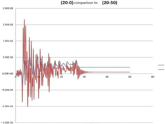
Figure 10.
Time functions of the total displacements for building top point in the X degree of freedom of height 20 m without soil (blue line) and for the same building with soil depth 50 m (red line). Horizontal axis: time in seconds, vertical axis: displacement in m.
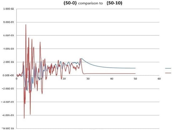
Figure 11.
Time functions of the total displacements for building top point in the X degree of freedom of height 50 m without soil (blue line) and for the same building with soil depth 10 m (red line). Horizontal axis: time in seconds, vertical axis: displacement in m.
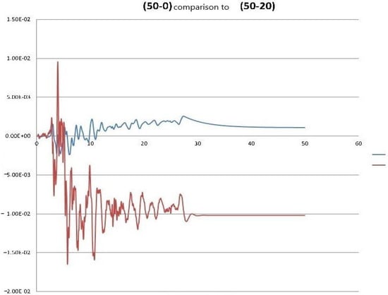
Figure 12.
Time functions of the total displacements for building top point in the X degree of freedom of height 50 m without soil (blue line) and for the same building with soil depth 20 m (red line). Horizontal axis: time in seconds, vertical axis: displacement in m.
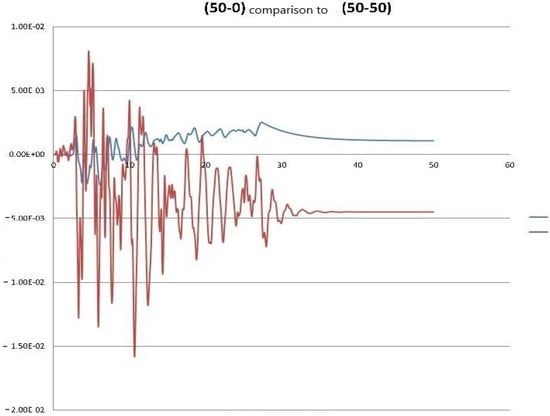
Figure 13.
Time functions of the total displacements for building top point in the X degree of freedom of height 50 m without soil (blue line) and for the same building with soil depth 50 m (red line). Horizontal axis: time in seconds, vertical axis: displacement in m.

Figure 14.
Time functions of the total acceleration for building top point in the X degree of freedom of height 10 m without soil (blue line) and for the same building with soil depth 10 m (red line). Horizontal axis: time in seconds, vertical axis: acceleration in .
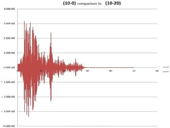
Figure 15.
Time functions of the total acceleration for building top point in the X degree of freedom of height 10 m without soil (blue line) and for the same building with soil depth 20 m (red line). Horizontal axis: time in seconds, vertical axis: acceleration in .

Figure 16.
Time functions of the total acceleration for building top point in the X degree of freedom of height 10 m without soil (blue line) and for the same building with soil depth 50 m (red line). Horizontal axis: time in seconds, vertical axis: acceleration in .
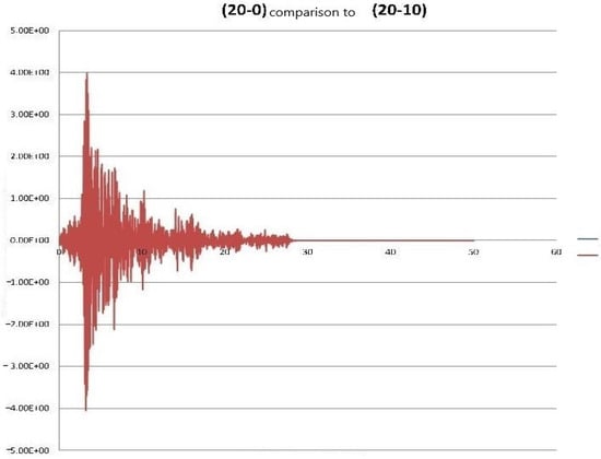
Figure 17.
Time functions of the total acceleration for building top point in the X degree of freedom of height 20 m without soil (blue line) and for the same building with soil depth 10 m (red line). Horizontal axis: time in seconds, vertical axis: acceleration in .
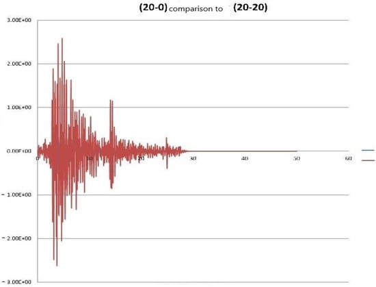
Figure 18.
Time functions of the total acceleration for building top point in the X degree of freedom of height 20 m without soil (blue line) and for the same building with soil depth 20 m (red line). Horizontal axis: time in seconds, vertical axis: acceleration in .
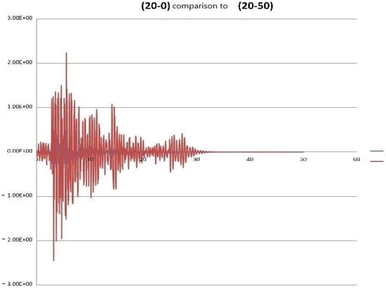
Figure 19.
Time functions of the total acceleration for building top point in the X degree of freedom of height 20 m without soil (blue line) and for the same building with soil depth 50 m (red line). Horizontal axis: time in seconds, vertical axis: acceleration in .
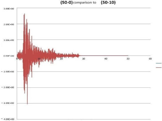
Figure 20.
Time functions of the total acceleration for building top point in the X degree of freedom of height 50 m without soil (blue line) and for the same building with soil depth 10 m (red line). Horizontal axis: time in seconds, vertical axis: acceleration in .
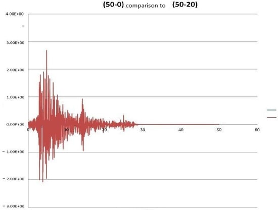
Figure 21.
Time functions of the total acceleration for building top point in the X degree of freedom of height 50 m without soil (blue line) and for the same building with soil depth 20 m (red line). Horizontal axis: time in seconds, vertical axis: acceleration in .
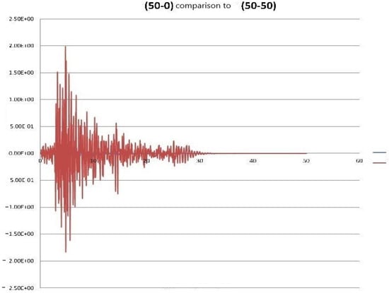
Figure 22.
Time functions of the total acceleration for building top point in the X degree of freedom of height 50 m without soil (blue line) and for the same building with soil depth 50 m (red line). Horizontal axis: time in seconds, vertical axis: acceleration in .
Table 5.
Peak values of the analyses for the residual and total displacements in meters, the total acceleration in and the ratio between the total and remaining displacements.
From the results obtained from the analyses, important deductions may be inferred for the dynamic soil–structure interactions for shear vulnerable structures subjected to palm loading. The residual total displacements, which occurred after the end of the earthquake, the greatest value is attained for the computational domain of the sole building of 10 m height, and is two orders of magnitude larger contrasted to the respective value for the soil with 50 m depth as portrayed in Figure 5, Figure 6 and Figure 7, and Table 5. For the SSI computational numerical model, for a building of 20 m height, the soil thickness of 20 m results in the greatest residual displacements as depicted in Figure 8, Figure 9 and Figure 10 and Table 5. This phenomenon takes place due to the soil resonance as a result of the frequency of the palm of Athens earthquake is approximately the eigenfrequency of the 20 m soil depth if it is considered as shear cantilever. In 10 m soil depth, due to the naivety of the model, the coarse FEM mesh and the following overestimation of the total stiffness a notable and unusual behaviour takes place. As the soil–structure interaction main identity, it is also evident here in all other occasions that the total displacement and residual displacement time history is larger when a soil is situated in the bottom of the superstructure in relation to the respective solution of the sole building. In 10 m soil depth, the largest displacements are obtained in the single building. For the ratio proposed in Table 5, referring to the proportion of total displacements to the residual ones, the minimum value is obtained in buildings with height 20 m when the soil depth is 20 m. This is also attained due to the fact of soil resonance of the subjected palm eigenfrequency. It is deducted that when a soil resonance is obtained, the ratio of the total to the residual displacements is lessened, since the denominator is enlarged.
The total displacement considering them as time functions for the building with height 10 m are mainly the same. That is, the trend of the response is similar when these smaller buildings are situated in the SSI computational system. Nevertheless, if the height of the superstructure is 20 m, a significant change in the time function takes place if the soil thickness is 20 m as portrayed in Figure 8, Figure 9 and Figure 10. Assuming that the superstructure height is 50 m the alteration takes place in soil thickness 20 m and 50 m, as depicted in Figure 11, Figure 12 and Figure 13. Combining this and the results obtained for the residual displacements, it may be concluded that the yield that took place in the superstructure of height 10 m has resulted in a significant alteration of the stiffness that changed also the displacement sign. The alteration of the trend of the total displacements may be attributed to the fact that the change in the stiffness of the superstructure result to a different energy flux distribution to the building, thus the output time function for the displacement response could not be the same. In all simulations performed, the damping is very intense, resulting in the transition from dynamic behaviour to residual displacements behaviour occurring in a very small time duration. As also observed from the time history analyses, and through the boundaries that are applied, no reflections of the seismic waves and consequently no standing waves took place. That leads to the conclusion that despite that the stiffness is overestimated; nonetheless, the damping is substantially estimated. In closing, the Athens Earthquake has a period domain of importance between 0.4 and 0.8 s. If a normal building is adopted the eigenperiod is approximated with the aid of an EC8 proposition as . Furthermore, the eigenvalue analysis of the building itself has given eigenvalues for the five different structures in the subset of eigenperiods [0.5, 0.75] in seconds. Subsequently, the resonance is evident. And analogous conclusions about the soil depth can be drawn.
The total top tip acceleration obtained for an SSI computational model is greater contrasted to the corresponding analyses of the sole building, as portrayed in Figure 14, Figure 15, Figure 16, Figure 17, Figure 18, Figure 19, Figure 20, Figure 21 and Figure 22 and Table 5. This contradicts the other SSI main identity about the SSI systems being more flexible contrasted to the respective ones that neglect the soil as sole buildings. Nevertheless, if a more fine FEM mesh is constituted, this trend tends to vanquish. Furthermore, the maximum acceleration is lessened when the soil depth is augmented in SSI models and when the building height is augmented for a sole superstructure. This is attributed to the fact that the power spectrum acceleration identity constitutes that to more flexible structures less acceleration is subjected to the body; subsequently, the aforementioned behaviour is justified. In all simulations, the time history function of the total tip accelerations is the same and only an amplification factor alters the respective time history output functions. That implies that the critical time when the flux is maximum and when the yield occurs is not influenced about the possible neglection of SSI. Moreover, this also implies that the energy flux in the top of the structure is not very much different and as a result the response of this degree of freedom is having the same trend regardless the possible reflections of the seismic waves to the top tip nodal degree of freedom.
An important perspective is also the computational effort and the effect of the nonlinear boundaries. The computational cost in relation to the respective linear analyses is at least 100%. In this article, for 1500 degrees of freedom, the solution time with direct integration is in the order of magnitude of 2 h. Nevertheless, with domain decomposition methods the analysis time may be drastically reduced about 50%. Furthermore, the nonlinear Lysmer boundaries are useful as checked in nonlinear analyses if the ratio width to depth is no more than 10. The analyses were conducted with the largest computational scheme and domain decomposition methods which proved to be the most efficient way of solving the presented numerical simulations. The aforementioned results are in accordance with the corresponding scientific publications literature [,], with the additional aspect that the analysis and the results are attained in a faster and more attested way. For concluding remarks, as the model number of nodal degrees of freedom is augmented, the scalability efficiency increases. Definitely, for the model constituting in the order of magnitude of 500 degrees of freedom, the direct solution has needed about 1:10 h (80 min). With domain decomposition schemes, the analysis time was reduced to 55 min; consequently, a 31.25% reduction in the time consumed for the deducted analysis occurred. The respective values for the largest computational domain of more than 1000 degrees of freedom are 2 h and 20 min (140 min) and 1 h and 10 min (70 min), which provides a 50% reduction in the time consumed for the analyses under discussion. It is expected that the percentage reduction after an increase and maximization will eventually lessened as the domain decomposition methods by themselves cannot speed-up the solution of the computational mechanics problem indefinitely. That scalability analysis for different domain decomposition methods with focusing on the most current algorithms proposed by the scientific community is an open subject for the dynamic soil–structure interaction analysis through the aid of the computational mechanics.
5. Conclusions
In the present article, a computational study of the dynamic soil–structure interaction effect on shear vulnerable structure is given. The loading is assumed as synchronous support excitation with the Lysmer energy-absorbing boundaries and the corresponding numerical problem to be solved. The constitutive stress–strain law is the Von Mises cylindrical yield function for a quantitatively accurate analysis, while the computational model solved can be considered as of high fidelity and complexity with about 1000 degrees of freedom to be addressed, through the Newmark integration scheme. The Athens 1999 earthquake is the excitation that is given to the soil mass, which is assumed as a palm force. This results to a numerical study that enlightens the soil–structure interaction phenomenon to palm seismic excitations, which are usually seen in the in situ world. The boundaries were investigated for their effect in the computational domain and the computational cost alleviation was also analysed with domain decompositions schemes and parallel computing algorithms with the use of open source numerical code MSolve.
In all simulations performed, the observed total displacements are greater with the soil–structure interaction system as expected. However, the observed total accelerations did not have the same trend; nevertheless, a more accurate model FEM model for the building vanquishes the aforementioned numerical abnormalities. Moreover, the largest acceleration is alleviated when the soil thickness increases in SSI systems and when the building height is greater for the sole structure. The residual displacement is in the order of magnitude of 0.008 m, which is fairly moderate as the inter storey drift is less than 1%. Nevertheless, the alteration of the residual displacement when the soil domain exists may be up to two orders of magnitude. In addition, it is deducted that a soil resonance in the case of soil depth 20 m is seen since the Athens earthquake period domain of importance is in between the estimated eigenperiod for the sole soil and the sole building. This results in a significant seismic energy flux, and this consequences to the maximum residual total displacements.
The conclusions from a computational point of view drawn from this study are notable. The increase in the computational cost was tackled with domain decomposition schemes and then a substantial alleviation of the time consumed for the analyses was observed. A domain reduction technique with the use of nonlinear Lysmer dashpots was also beneficial and, subsequently, the computational scheme implementation is more efficient compared to the direct computational domain integration. It is portrayed that parallel computing and domain decomposition systems are a complex, but efficient, way to speed up the computational mechanics problems solution. Nevertheless, a less complex way for moderate number of degrees of freedom may also be implemented. Finally, in geomechanics, the development of the aforementioned methods may postulate an easier and more accurate prediction of the SSI response, which leads to a more economic design and gives data for Artificial Intelligence and Machine Learning applications in sciences and engineering.
In conclusion, future research in the discussed scientific field is available in several parts of the analysis conducted. At first, the building simulation may be with more complexity used hexahedral finite elements. Alternatively, there is the possibility to interpreter the building using Force Based Distributed Plasticity beam elements that follow the Timoshenko beam for the displacement field [,]. Moreover, for the soil computational domain, apart from a more fine FEM mesh in order to increase the computational accuracy, a selection of a more accurate constitutive material model can be incorporated such as the Drucker–Prager model, among others, which is in the scope of the author of this manuscript. Finally, the selection of alternative energy absorption dashpots like the ones analysed in Introduction is also possible.
Funding
This research has been supported by REGALE An open architecture to equip next generation HPC applications with exascale capabilities H2020 from the European Union.
Data Availability Statement
The raw data supporting the conclusions of this article will be made available by the authors on request because of the magnitude and perplexity of the raw data files. Open source code MSolve in programming Language C# is used for the analyses. Information can be found at the following link: http://mgroup.ntua.gr/, accessed on 28 June 2024.
Conflicts of Interest
The author declares no conflicts of interest.
References
- Mylonakis, G.; Gazetas, G. Seismic soils tructure interaction: Beneficial or Detrimental? J. Earthq. Eng. 2000, 4, 277–301. [Google Scholar] [CrossRef]
- Wegner, J.; Yao, M.; Zhang, X. Dynamic wave–soil–structure interaction analysis in the time domain. Comput. Struct. 2005, 83, 2206–2214. [Google Scholar] [CrossRef]
- Saouma, V.; Miura, F.; Lebon, G.; Yagome, Y. A simplified 3D model for soil-structure interaction with radiation damping and free field input. Bull. Earthq. Eng. 2011, 9, 1387–1402. [Google Scholar] [CrossRef]
- Wang, G.; Wang, Y.; Pan, P.; Wang, J. Experimental and numerical investigation on seismic response of the soil-structure cluster interaction system. Eng. Struct. 2023, 285, 116001. [Google Scholar] [CrossRef]
- Zucca, M.; Crespi, P.G.; Longarini, N. Seismic vulnerability assessment of an Italian historical masonry dry dock. Case Stud. Struct. Eng. 2017, 7, 1–23. [Google Scholar] [CrossRef]
- Dong, J.; Niu, Z.; Li, J.; Hong, G.; Pan, J.; Li, H. System identification of excited beam immersed in granular materials: A multifrequency data-based method in a variational framework. Eng. Struct. 2023, 293, 116611. [Google Scholar] [CrossRef]
- Chen, S.S.; Hou, J.G. Response of circular flexible foundations subjected to horizontal and rocking motions. Soil Dyn. Earthq. Eng. 2015, 69, 182–195. [Google Scholar] [CrossRef]
- Sheng, T.; Liu, G.B.; Bian, X.C.; Shi, W.X.; Chen, Y. Development of a three-directional vibration isolator for buildings subject to metro- and earthquake-induced vibrations. Eng. Struct. 2022, 252, 113576. [Google Scholar] [CrossRef]
- Zucca, M.; Valente, M. On the limitations of decoupled approach for the seismic behaviour evaluation of shallow multi-propped underground structures embedded in granular soils. Eng. Struct. 2020, 211, 110497. [Google Scholar] [CrossRef]
- Connolly, D.P.; Marecki, G.P.; Kouroussis, G.; Thalassinakis, I.; Woodward, P.K. The growth of railway ground vibration problems — A review. Sci. Total Environ. 2016, 568, 1276–1282. [Google Scholar] [CrossRef]
- Kavvadas, M.; Amorosi, A. A constitutive model for structured soils. Geotechnique 2000, 50, 263–273. [Google Scholar] [CrossRef]
- Savvides, A.; Papadrakakis, M. A computational study on the uncertainty quantification of failure of clays with a modified Cam-Clay yield criterion. Springer Nat. Appl. Sci. 2021, 3, 659. [Google Scholar] [CrossRef]
- Savvides, A.; Papadopoulos, L. A Neural Network Model for Estimation of Failure Stresses and Strains in Cohesive Soils. Geotechnics 2022, 2, 1084–1108. [Google Scholar] [CrossRef]
- İmamoğlu, Ç.; Dicleli, M. Effect of dynamic soil-structure interaction modeling assumptions on the calculated seismic response of railway bridges with single-column piers resting on shallow foundations. Soil Dyn. Earthq. Eng. 2024, 181, 108624. [Google Scholar] [CrossRef]
- Korre, E.; Zeghal, M.; Abdoun, T. Liquefaction in the presence of soil-structure interaction: Centrifuge tests of a sheet-pile quay wall in LEAP-2020. Soil Dyn. Earthq. Eng. 2024, 181, 108650. [Google Scholar] [CrossRef]
- Wu, Y.; Zhao, M.; Gao, Z.; Du, X. Seismic performance analysis of structure equipped with tuned mass dampers considering nonlinear soil-structure interaction effects. Structures 2024, 63, 106425. [Google Scholar] [CrossRef]
- Liu, B.; Xue, J.; Lehane, B.M.; Yin, Z.Y. Time-dependent soil–structure interaction analysis using a macro-element foundation model. Eng. Struct. 2024, 308, 118046. [Google Scholar] [CrossRef]
- Abdulaziz, M.A.; Hamood, M.J.; Fattah, M.Y. Investigating seismic behavior in adjacent structures: A study on the impact of structures embedment level and existence of dead loads considering soil-structure interaction. Results Eng. 2024, 22, 102023. [Google Scholar] [CrossRef]
- Ocak, A.; Melih Nigdeli, S.; Bekdaş, G. Optimization of the base isolator systems by considering the soil-structure interaction via metaheuristic algorithms. Structures 2023, 56, 104886. [Google Scholar] [CrossRef]
- Forcellini, D. The role of Soil Structure Interaction (SSI) on the risk of pounding between low-rise buildings. Structures 2023, 56, 105014. [Google Scholar] [CrossRef]
- Abdulaziz, M.A.; Hamood, M.J.; Fattah, M.Y. A review study on seismic behavior of individual and adjacent structures considering the soil – Structure interaction. Structures 2023, 52, 348–369. [Google Scholar] [CrossRef]
- Genç, A.F.; Atmaca, E.E.; Günaydin, M.; Altunişik, A.C.; Sevim, B. Evaluation of soil structure interaction effects on structural performance of historical masonry buildings considering earthquake input models. Structures 2023, 54, 869–889. [Google Scholar] [CrossRef]
- Shang, H.; Bao, C.; Wang, H.; Ma, X.; Cao, J.; Du, J. Seismic response analysis of frame structures with uneven settlement of foundation considering soil-structure interaction. Results Eng. 2023, 20, 101574. [Google Scholar] [CrossRef]
- Cheng, F.; Li, J.; Zhou, L.; Lin, G. Fragility analysis of nuclear power plant structure under real and spectrum-compatible seismic waves considering soil-structure interaction effect. Eng. Struct. 2023, 280, 115684. [Google Scholar] [CrossRef]
- Han, Q.; Wu, C.; Liu, M.; Wu, H. Corotational isogeometric shear deformable geometrically exact spatial form beam element for general large deformation analysis of flexible thin-walled beam structures. Thin-Walled Struct. 2024, 198, 111684. [Google Scholar] [CrossRef]
- Bielak, J.; Christiano, P. On the effective seismic input for non-linear soil-structure interaction systems. Earthq. Eng. Struct. Dyn. 1984, 12, 107–119. [Google Scholar] [CrossRef]
- Ceremonini, M.; Christiano, P.; Bielak, J. Implementation of effective seismic input for soil-structure interaction systems. Earthq. Eng. Struct. Dyn. 1988, 16, 615–625. [Google Scholar] [CrossRef]
- Zhang, Y.; Yang, Z.; Bielak, J.; Conte, P.; Elgamal, A.W. Treatment of seismic input and boundary conditions in nonlinear seismic analysis of a bridge ground system. In Proceedings of the Conference: 16-th ASCE Engineering Mechanics Conference, Seattle, WA, USA, 16–18 July 2003; University of Washington: Seattle, WA, USA, 2003. [Google Scholar]
- Fattah, M.Y. A New Mapped Infinite Element for Dynamic Analysis of Soil-Structure Interaction Problems. Diyala J. Eng. Sci. 2010, 327–355. [Google Scholar]
- Fattah, M.Y.; Hamood, M.J.; Dawood, S.H. Dynamic Analysis of Soil-Structure Interaction Problems Considering Infinite Boundaries. Eng. Technol. J. Univ. Technol. 2008, 26, 725–746. [Google Scholar] [CrossRef]
- Fattah, M.Y.; Hamood, M.J.; Dawood, S.H. Dynamic Response of a Lined Tunnel with Transmitting Boundaries. Earthq. Struct. 2015, 8, 275–304. [Google Scholar] [CrossRef]
- Abdulrasool, A.S.; Fattah, M.Y.; Salim, N.M. Application of Energy Absorbing Layer to Soil-structure Interaction Analysis. IOP Conf. Ser. Mater. Sci. Eng. 2020, 737, 012094. [Google Scholar] [CrossRef]
- Tullini, N.; Tralli, A. Static analysis of Timoshenko beam resting on elastic half-plane based on the coupling of locking-free finite elements and boundary integral. Comput. Mech. 2010, 45, 211–225. [Google Scholar] [CrossRef]
- Baraldi, D.; Tullini, N. In-plane bending of Timoshenko beams in bilateral frictionless contact with an elastic half-space using a coupled FE-BIE method. Eng. Anal. Bound. Elem. 2018, 97, 114–130. [Google Scholar] [CrossRef]
- Baraldi, D.; Tullini, N. Static stiffness of rigid foundation resting on elastic half-space using a Galerkin boundary element method. Eng. Struct. 2020, 225, 111061. [Google Scholar] [CrossRef]
- Hu, Z.P.; Pan, W.H.; Tong, J.Z. Exact Solutions for Buckling and Second-Order Effect of Shear Deformable Timoshenko Beam–Columns Based on Matrix Structural Analysis. Appl. Sci. 2019, 9, 3814. [Google Scholar] [CrossRef]
- Choi, M.J.; Cho, S. Isogeometric configuration design sensitivity analysis of geometrically exact shear-deformable beam structures. Comput. Methods Appl. Mech. Eng. 2019, 351, 153–183. [Google Scholar] [CrossRef]
- Banić, D.; Turkalj, G.; Lanc, D. Stability analysis of shear deformable cross-ply laminated composite beam-type structures. Compos. Struct. 2023, 303, 116270. [Google Scholar] [CrossRef]
- Reddy, J. On locking-free shear deformable beam finite elements. Comput. Methods Appl. Mech. Eng. 1997, 149, 113–132. [Google Scholar] [CrossRef]
- Challamel, N.; Elishakoff, I. A brief history of first-order shear-deformable beam and plate models. Mech. Res. Commun. 2019, 102, 103389. [Google Scholar] [CrossRef]
- Thatikonda, N.P.; Baraldi, D.; Boscato, G.; Cecchi, A. Experimental evaluation of elastic shear components for masonry in a Cosserat Continuum. Int. J. Solids Struct. 2024, 292, 112715. [Google Scholar] [CrossRef]
- Elmeligy, O.; AbdelRahman, B.; Galal, K. Experimental investigation of the compressive and shear behaviours of grouted and hollow masonry constructed with PVA fibre-reinforced mortar and grout. Constr. Build. Mater. 2024, 415, 134954. [Google Scholar] [CrossRef]
- Wang, B.; Yin, S.; Qu, F.; Wang, F. Cyclic shear test and finite element analysis of TRC-reinforced damaged confined masonry walls. Constr. Build. Mater. 2024, 421, 135766. [Google Scholar] [CrossRef]
- Namlı, M.; Aras, F. Performance evaluation of a seismic strengthening applied on a masonry school building by dynamic analyses. Structures 2024, 62, 106200. [Google Scholar] [CrossRef]
- Silvestri, F.; de Silva, F.; Piro, A.; Parisi, F. Soil-structure interaction effects on out-of-plane seismic response and damage of masonry buildings with shallow foundations. Soil Dyn. Earthq. Eng. 2024, 177, 108403. [Google Scholar] [CrossRef]
- de Araújo, F.C.; Ribeiro, I.S.; Machado, R.M. Nonlinear analysis of semirigid steel frames having nonprismatic shear-deformable members. Eng. Struct. 2022, 257, 114047. [Google Scholar] [CrossRef]
- Qiu, Z.; Deng, M.; Tian, X.; Li, T.; Sun, H.; Cao, J. Experimental study and theoretical analysis on steel frames infilled high-ductility concrete shear walls. Constr. Build. Mater. 2024, 434, 136739. [Google Scholar] [CrossRef]
- Moeinifard, P.; Ghiami Azad, A.R.; Mirghaderi, S.R. Numerical comparison of truss-shaped lateral load-resisting systems with conventional steel shear walls. Structures 2024, 62, 106261. [Google Scholar] [CrossRef]
- He, M.; Zhang, Q.; Sun, X.; Alhaddad, W. An experimental and numerical study on the shear performance of friction-type high-strength bolted connections used for CLT-steel hybrid shear walls. Eng. Struct. 2024, 306, 117868. [Google Scholar] [CrossRef]
- Jiang, Z.Q.; Wang, J.J.; Shen, C.J.; Yan, T.; Su, L. Cyclic loading behavior of novel internally stiffened double steel plate shear wall. J. Build. Eng. 2024, 90, 109462. [Google Scholar] [CrossRef]
- Zimos, D.K.; Mergos, P.E.; Papanikolaou, V.K.; Kappos, A.J. Analysis of shear-critical reinforced concrete columns under variable axial load. Mag. Concr. Res. 2022, 74, 715–726. [Google Scholar] [CrossRef]
- Liang, D.; Xue, F. Integrating automated machine learning and interpretability analysis in architecture, engineering and construction industry: A case of identifying failure modes of reinforced concrete shear walls. Comput. Ind. 2023, 147, 103883. [Google Scholar] [CrossRef]
- Ivanov, M.L.; Chow, W.K. Structural damage observed in reinforced concrete buildings in Adiyaman during the 2023 Turkiye Kahramanmaras Earthquakes. Structures 2023, 58, 105578. [Google Scholar] [CrossRef]
- El-Azizy, O.A.; Ezzeldin, M.; El-Dakhakhni, W. Comparative analyses of reinforced masonry and reinforced concrete shear walls with different end configurations: Seismic performance and economic assessment. Eng. Struct. 2023, 296, 116852. [Google Scholar] [CrossRef]
- Yamada, H.; Yamada, R.; Tani, M.; Nishiyama, M. Damage evaluation for reinforced concrete shear walls via motion capture and optical fiber sensors. Structures 2024, 60, 105955. [Google Scholar] [CrossRef]
- MIDAS Users Manual. Available online: https://manual.midasuser.com/en_common/GTS%20NX/150/GTS_NX/Mesh/Property,Coordinate,Function/Material/General_Material(Behavioral_properties)/von_Mises.htm (accessed on 29 June 2024).
- Roscoe, K.; Schofield, A.; Thurairajah, A. Laboratory shear testing of soils: An Evaluation of Test Data for Selecting a Yield Criterion for Soils. In The Symposium on Laboratory Shear Testing of Soils, ASTM Committee D18 on Soils for Engineering Purposes and the National Research Council of Canada; ASTM International: West Conshohocken, PA, USA, 1963; Volume 1. [Google Scholar]
- Chakraborty, D.; Kumar, J. Use of von Mises yield criterion for solving axisymmetric stability problems. Geomech. Geoeng. 2015, 10, 234–241. [Google Scholar] [CrossRef]
- Newmark, N.M. A method of computation for structural dynamics. J. Eng. Mech. Div. 1959, 85, 67–94. Available online: https://engineering.purdue.edu/~ce573/Documents/Newmark_A%20Method%20of%20Computation%20for%20Structural%20Dynamics.pdf (accessed on 29 June 2024).
- Simo, J.; Tarnow, N.; Wong, K. Exact energy-momentum conserving algorithms and symplectic schemes for nonlinear dynamics. Comput. Methods Appl. Mech. Eng. 1992, 100, 63–116. [Google Scholar] [CrossRef]
- Chang, S.Y. A technique for overcoming load discontinuity in using Newmark method. J. Sound Vib. 2007, 304, 556–569. [Google Scholar] [CrossRef]
- Lysmer, J.; Kuhlemeyer, R.L. Finite dynamic model for infinite media. ASCE J. Eng. Mech. Div. 1969, 95, 859–877. [Google Scholar] [CrossRef]
- Lekkas, E. The Athens earthquake (7 September 1999): Intensity distribution and controlling factors. Eng. Geol. 2001, 59, 297–311. [Google Scholar] [CrossRef]
- Mylonakis, G.; Voyagaki, E.; Price, T. Damage Potential of the 1999 Athens, Greece, Accelerograms. Bull. Earthq. Eng. 2003, 1, 205–240. [Google Scholar] [CrossRef]
- Renzi, S.; Madiai, C.; Vanucchi, G. A simplified empirical method for assessing seismic soil-structure interaction effects on ordinary shear-type buildings. Soil Dyn. Earthq. Eng. 2013, 55, 100–107. [Google Scholar] [CrossRef]
- Taucer, F.; Spacone, E.; Filippou, F. A Fiber Beam-Column Element for Seismic Response Analysis of Reinforced Concrete Structures; Earthquake Engineering Research Center, College of Engineering, University of California: Berkeley, CA, USA, 1991. [Google Scholar]
- Papachristidis, A.; Fragiadakis, M.; Papadrakakis, M. A 3D fibre beam-column element with shear modelling for the inelastic analysis of steel structures. Comput. Mech. 2010, 45, 553–572. [Google Scholar] [CrossRef]
Disclaimer/Publisher’s Note: The statements, opinions and data contained in all publications are solely those of the individual author(s) and contributor(s) and not of MDPI and/or the editor(s). MDPI and/or the editor(s) disclaim responsibility for any injury to people or property resulting from any ideas, methods, instructions or products referred to in the content. |
© 2024 by the author. Licensee MDPI, Basel, Switzerland. This article is an open access article distributed under the terms and conditions of the Creative Commons Attribution (CC BY) license (https://creativecommons.org/licenses/by/4.0/).