
A Microscale Framework for Seismic Stability Analysis of Bridge Pier Rocking Isolation Using the Discrete Element Method

Abstract
:1. Introduction
2. Materials and Methods
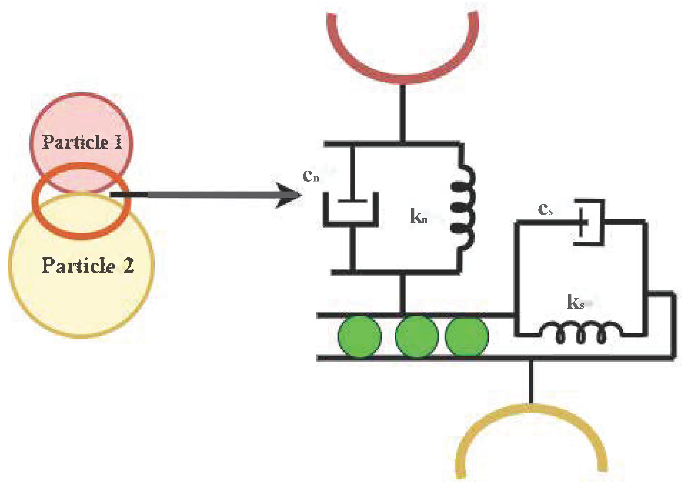
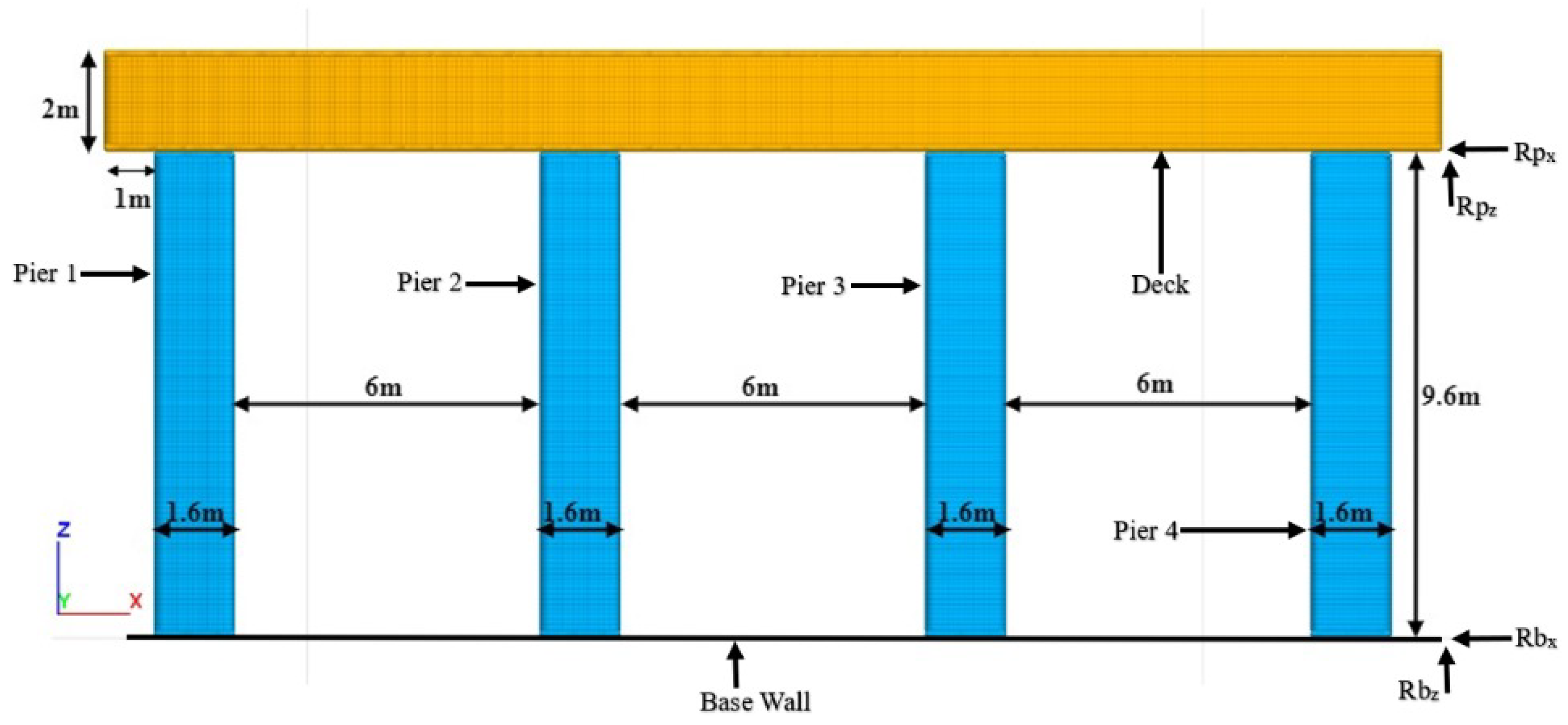
2.1. Computational Model
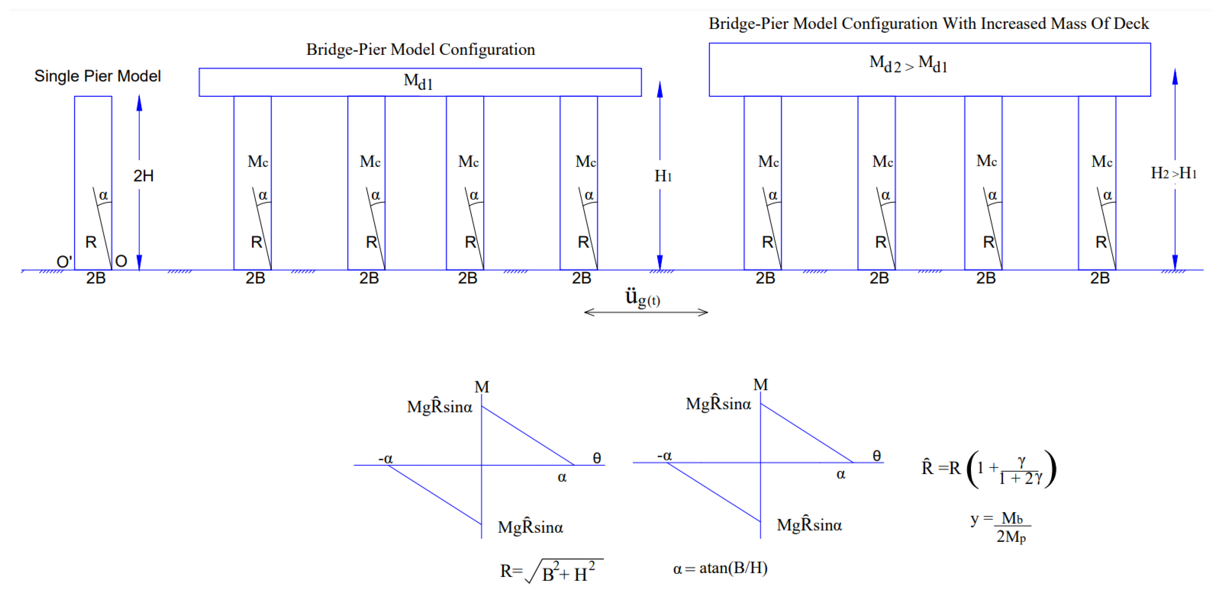
2.2. Model of a Rigid Body Formulation
2.3. Full Equations of Motion for a Rigid Body
- Set .
- Set equal to the initial angular velocity (i.e., before the motion computation).
- Solve Equation (24) for .
- Determine a new (provisional) angular velocity, assuming no damping:
- Revise the estimate of as
- Set and go to Step 3.
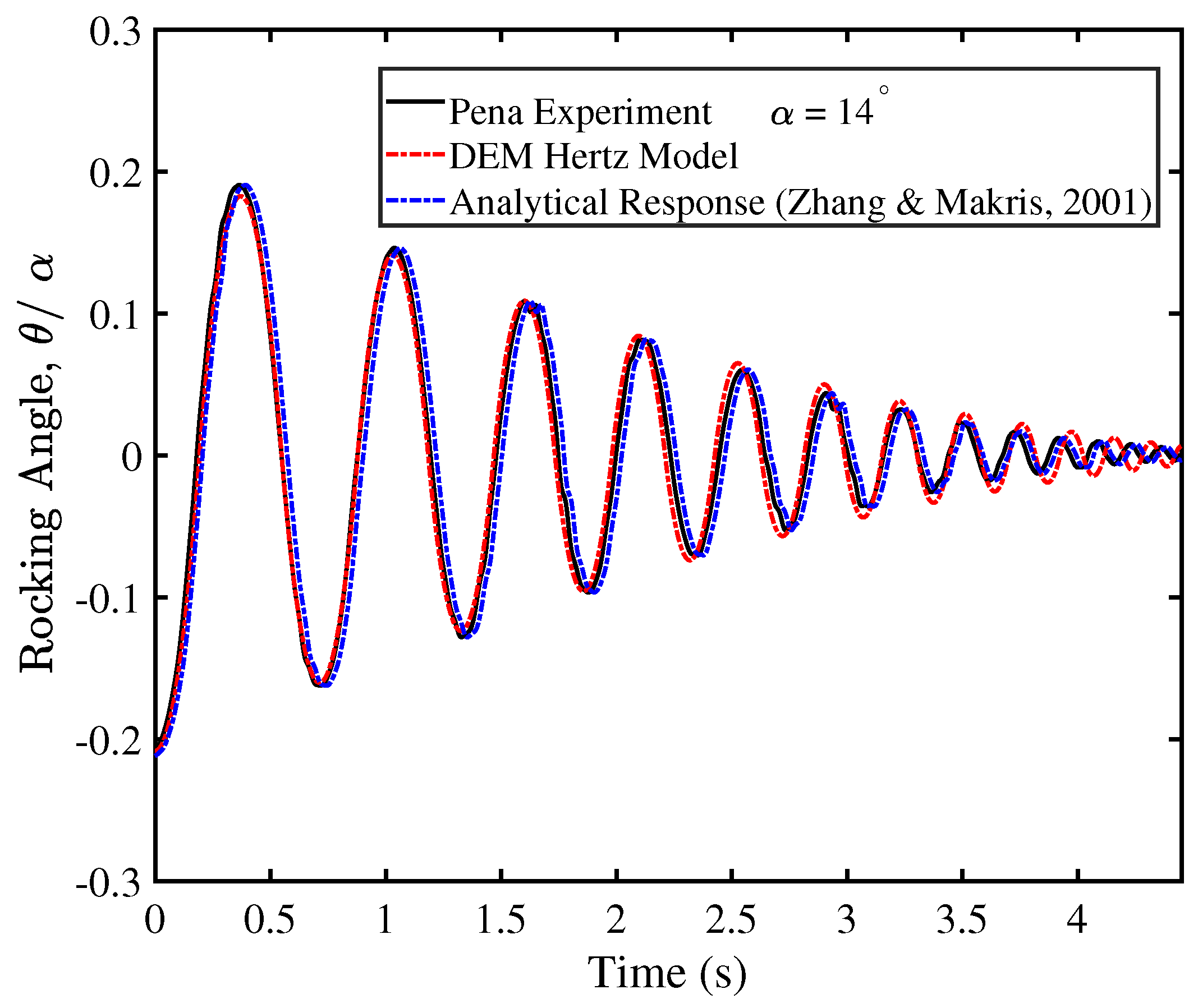
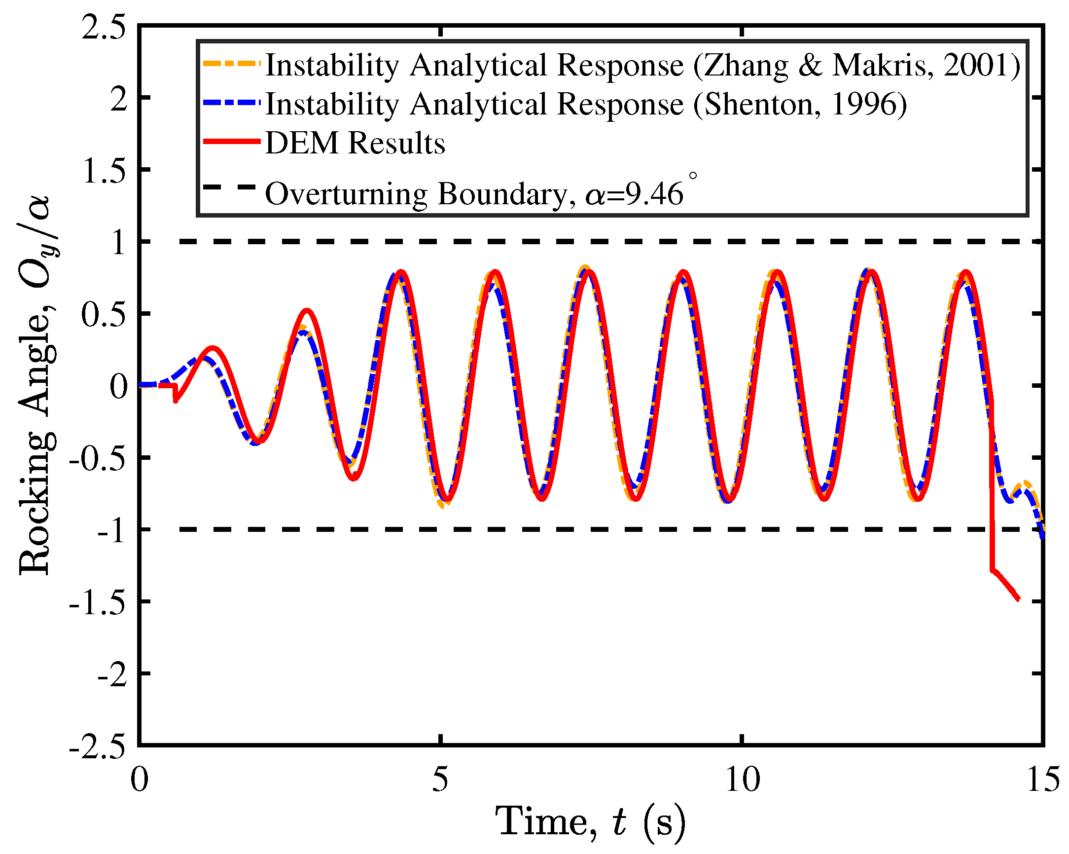
3. Validation
4. Results
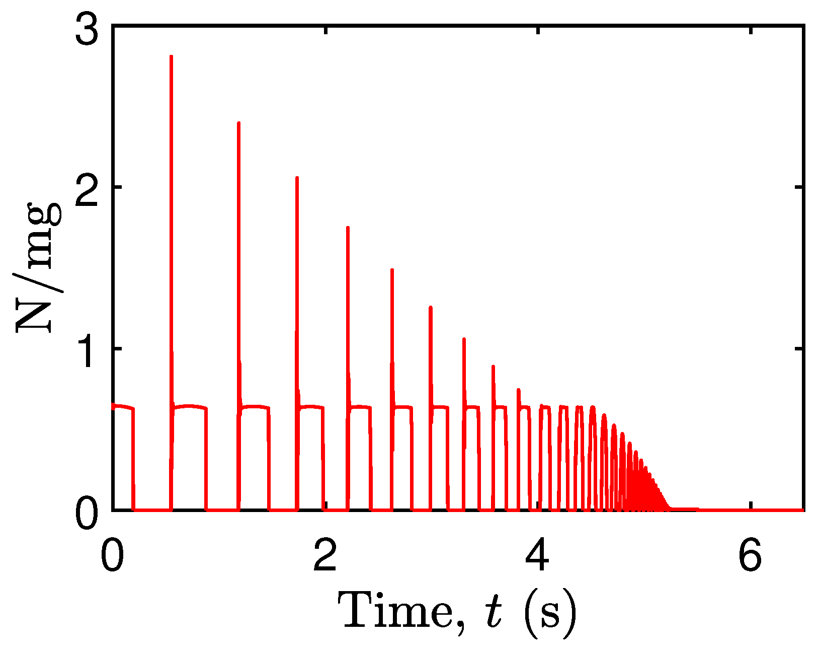
4.1. Contact Mechanics in a Free-Standing Rigid Block
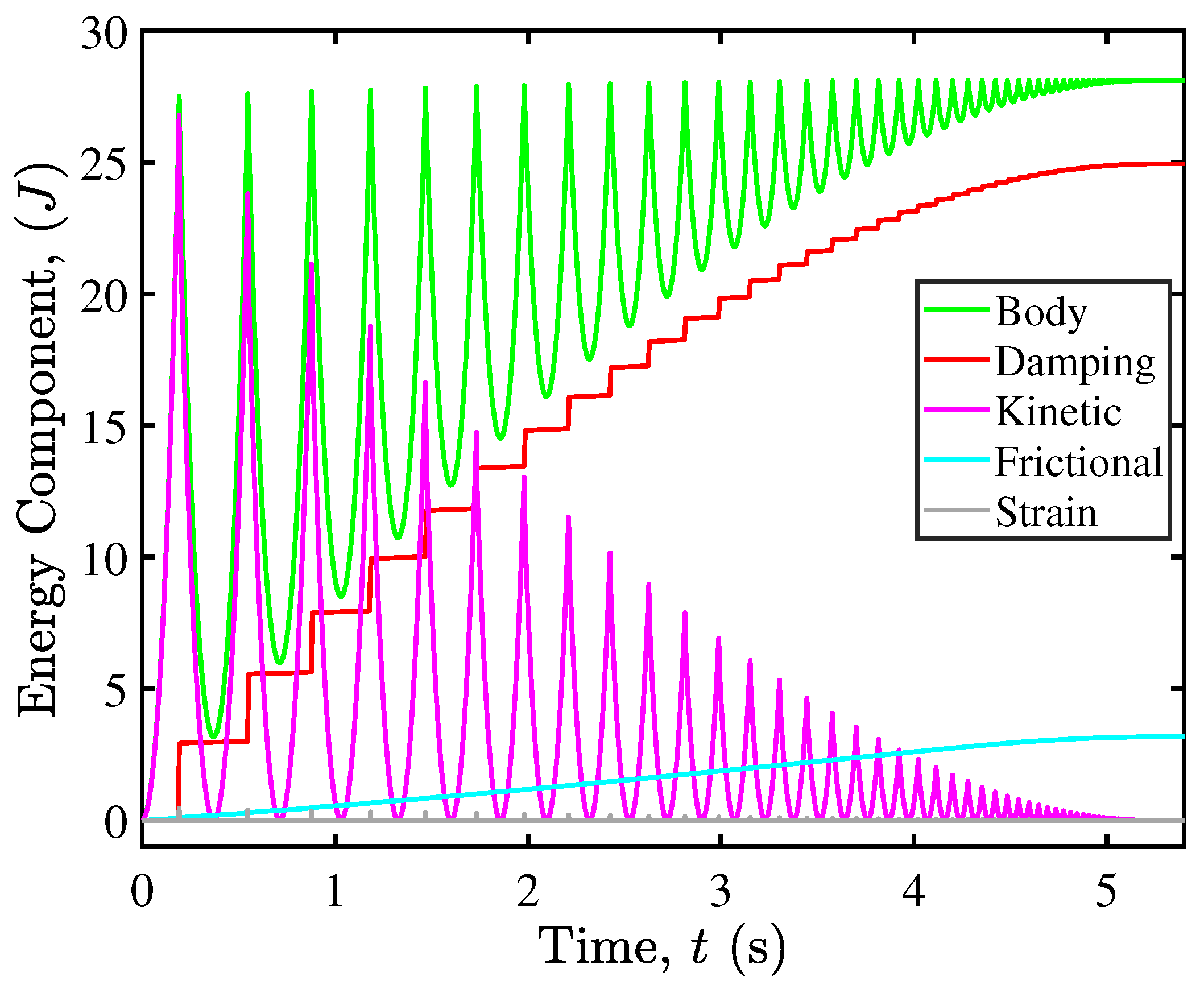
4.2. Microscale Energy Monitoring and Dissipation Mechanism
5. Seismic Isolation of Rocking Bridge Pier Structures
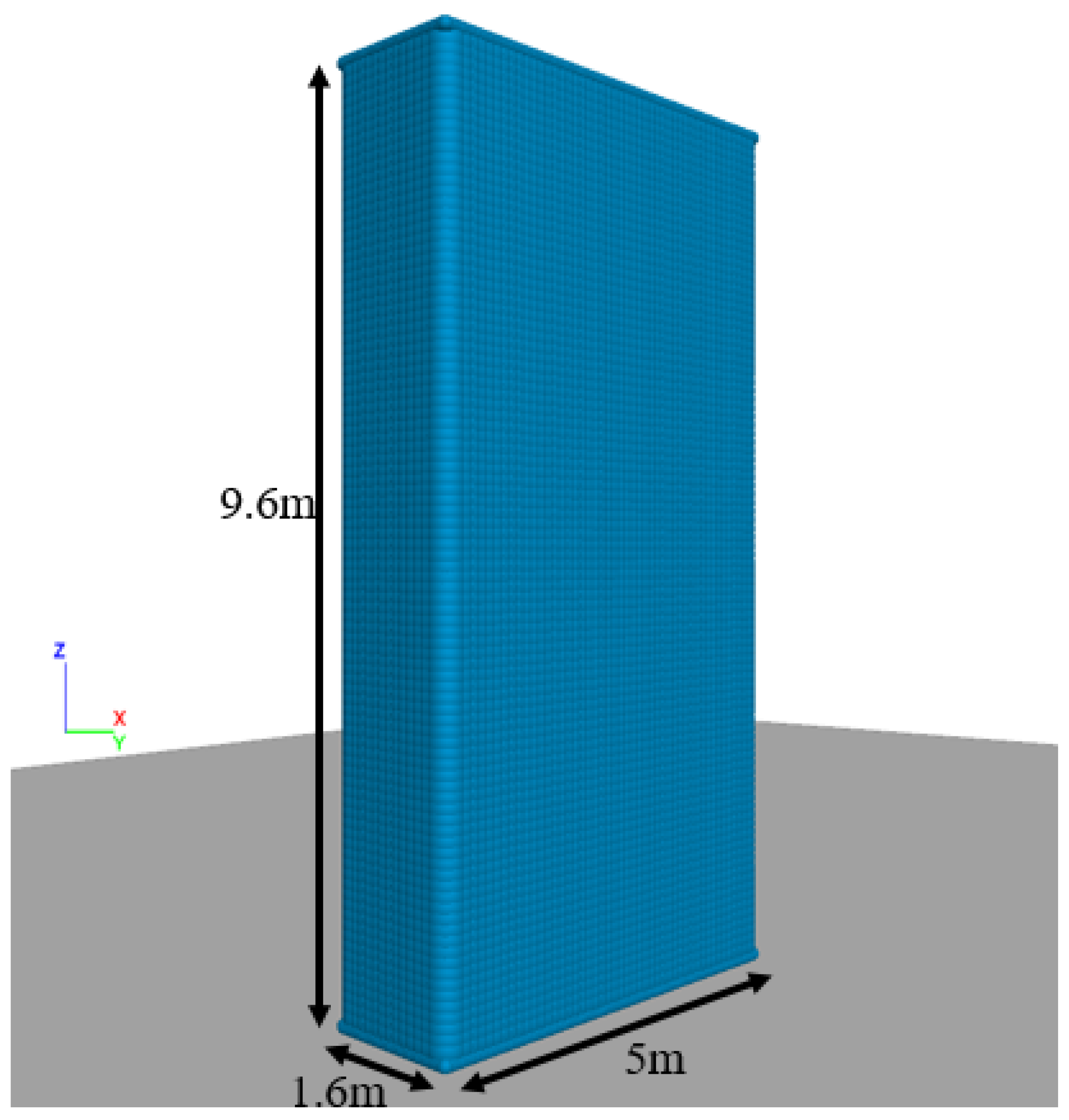
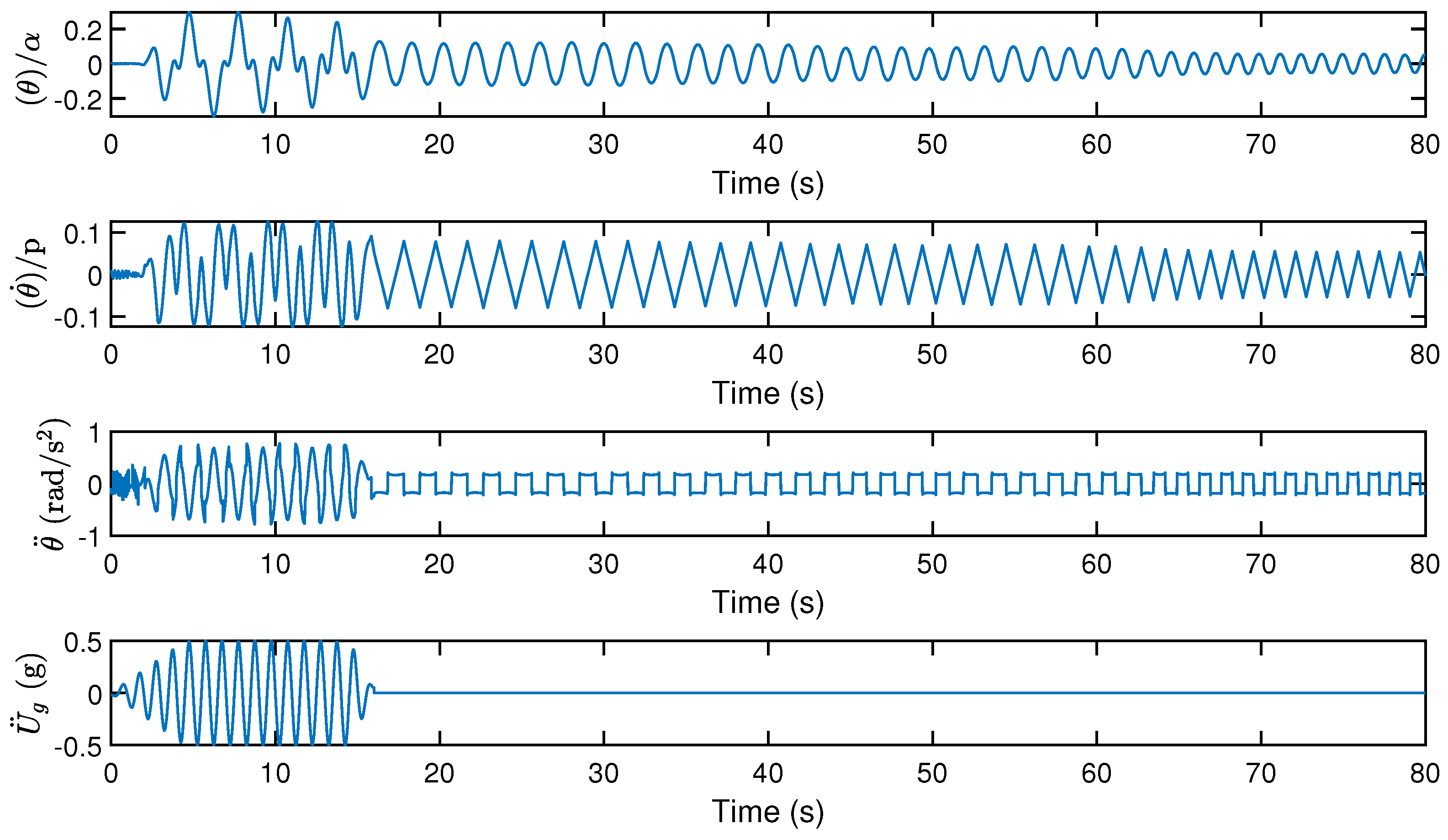
5.1. Seismic Response of a Single-Pier
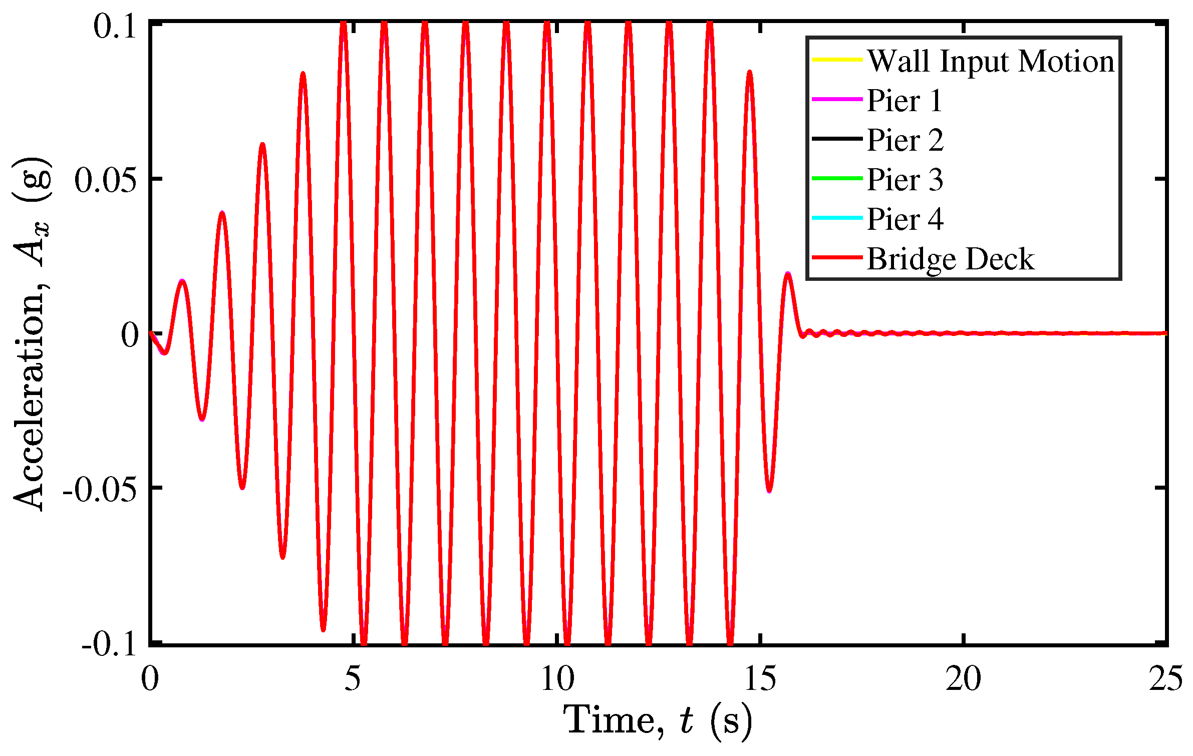
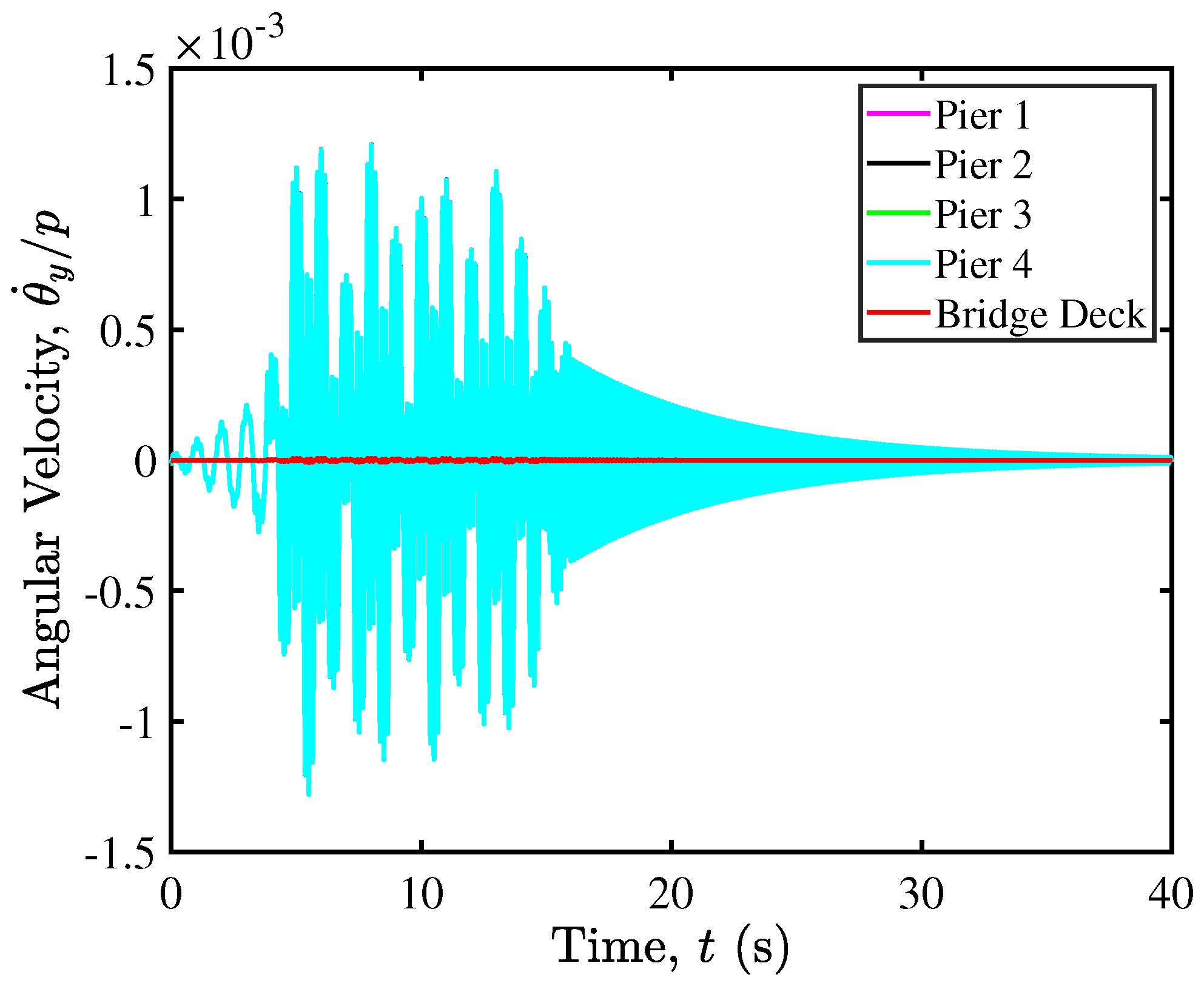
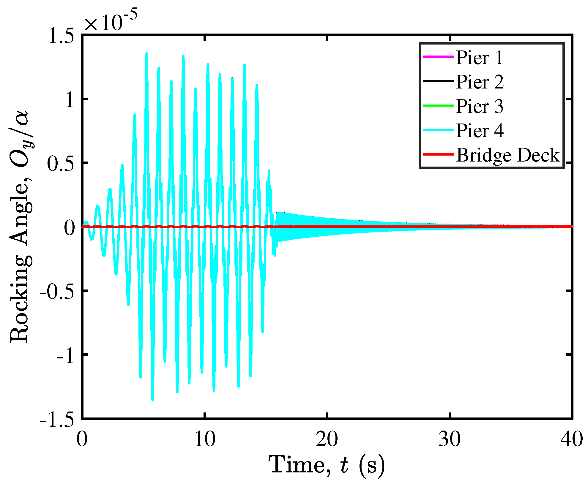
5.2. Rocking Isolation in Pier–Deck Systems under Low-Intensity Seismic Excitation
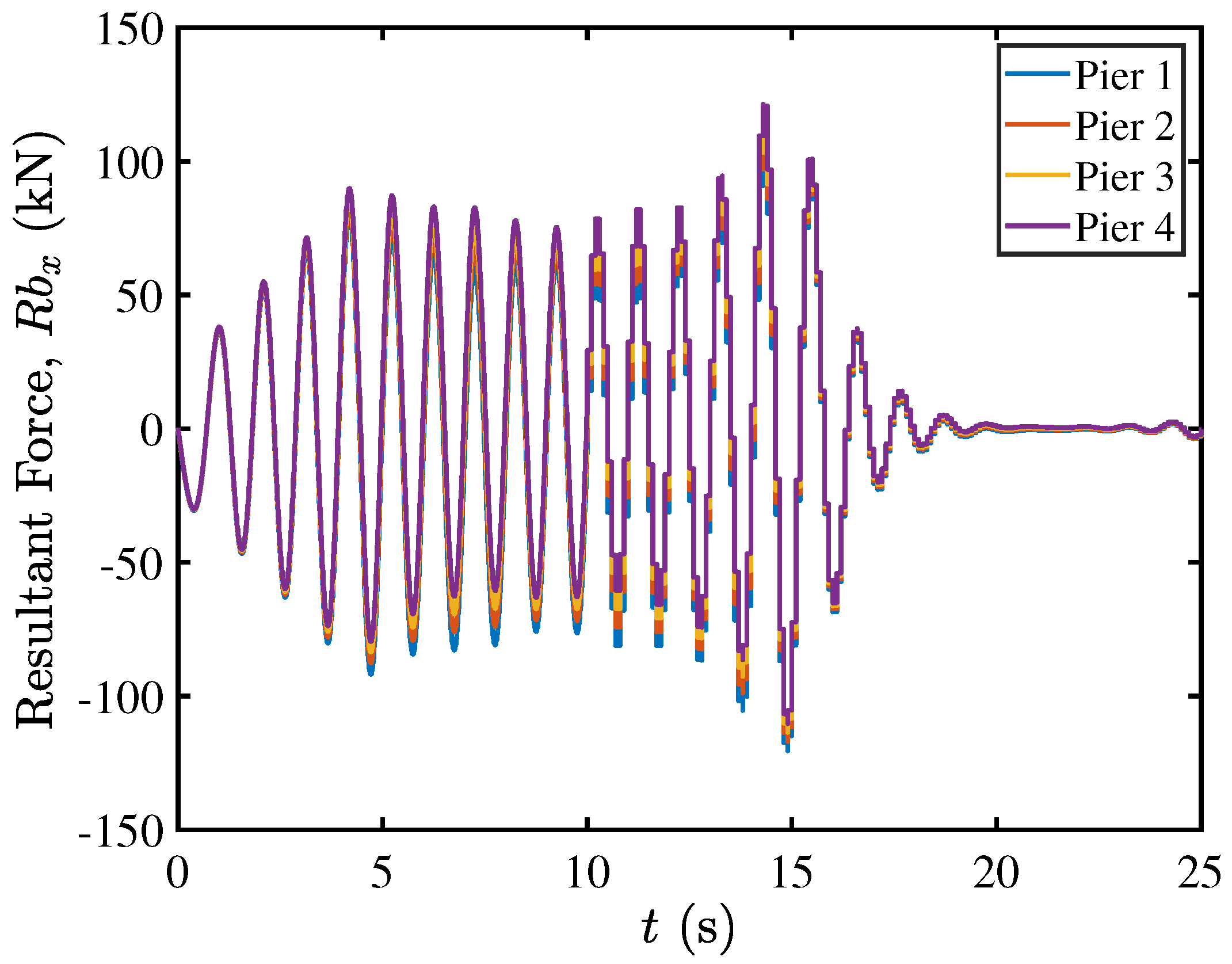
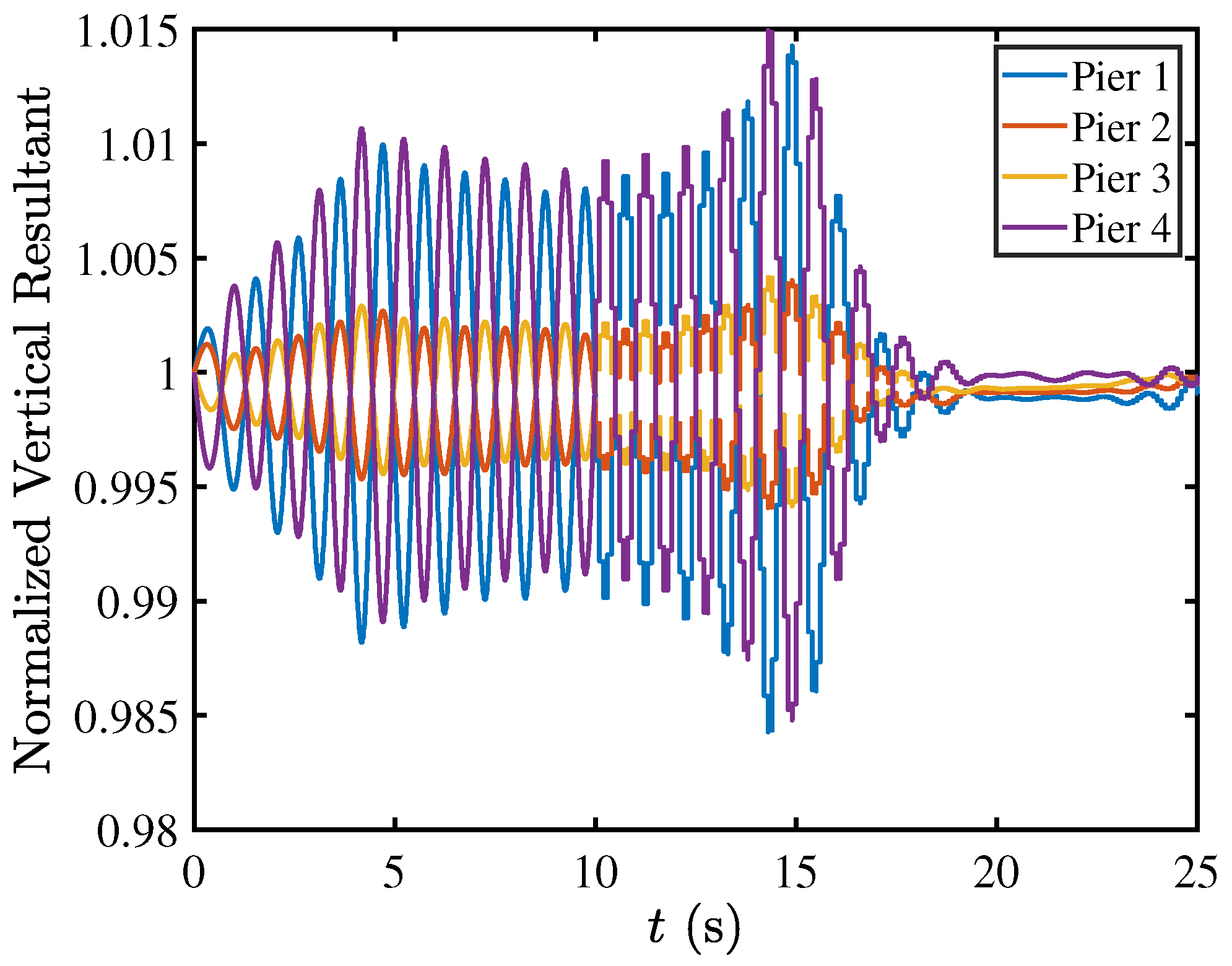
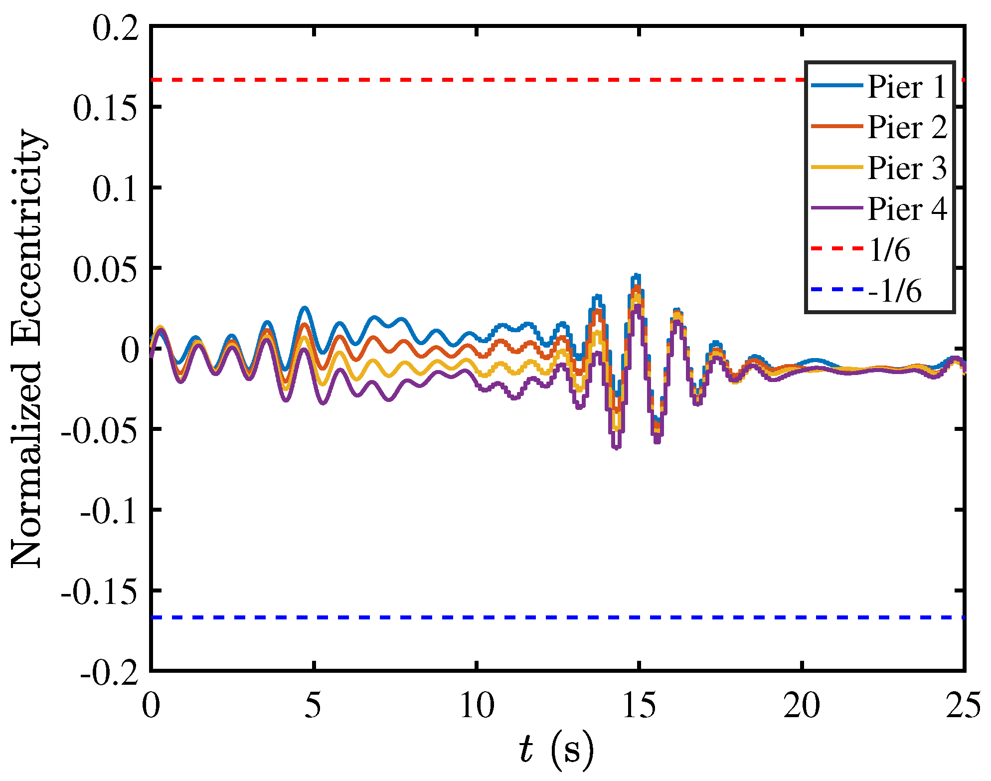
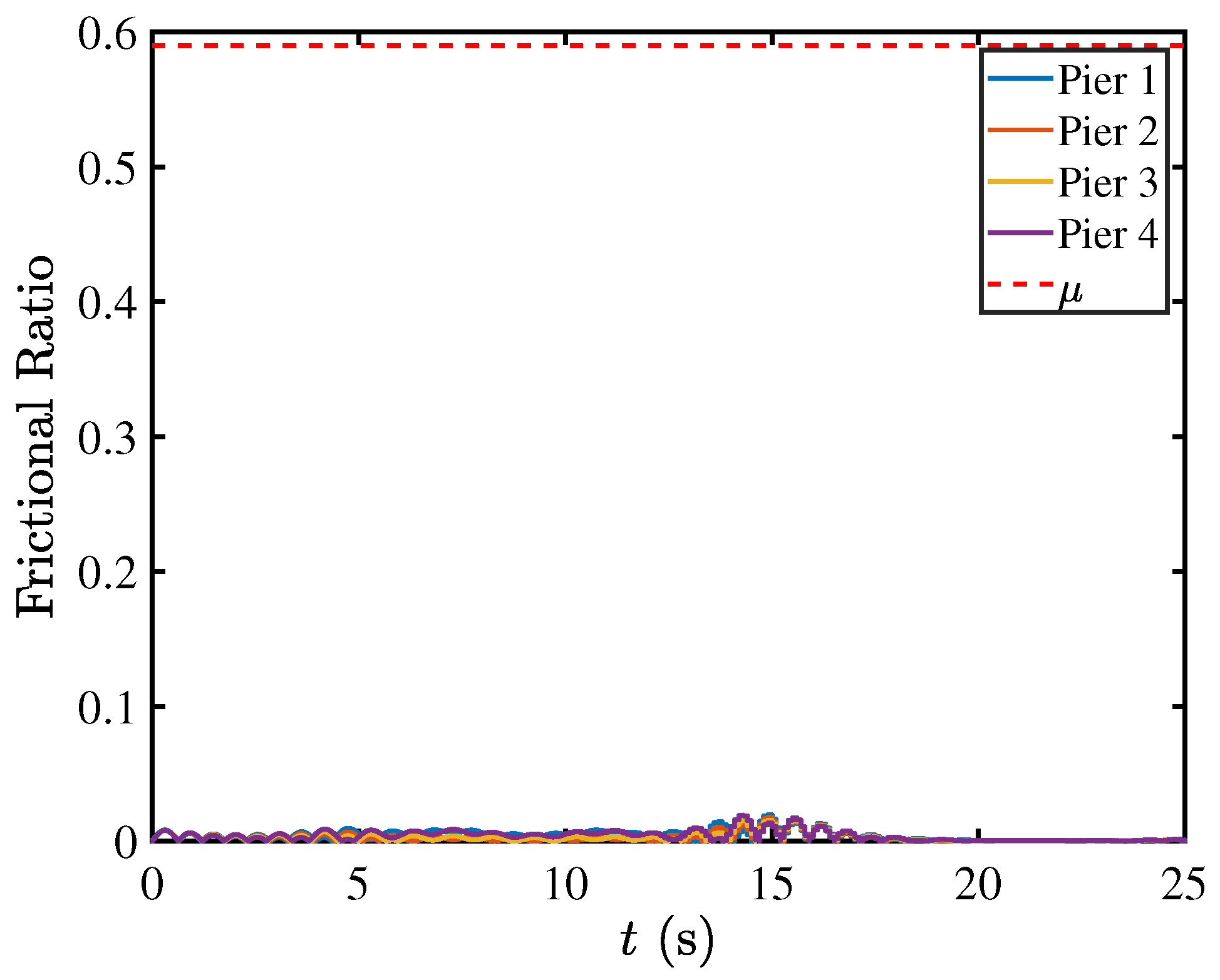
5.3. Contact Mechanics in Pier–Deck System under Low-Intensity Seismic Excitation
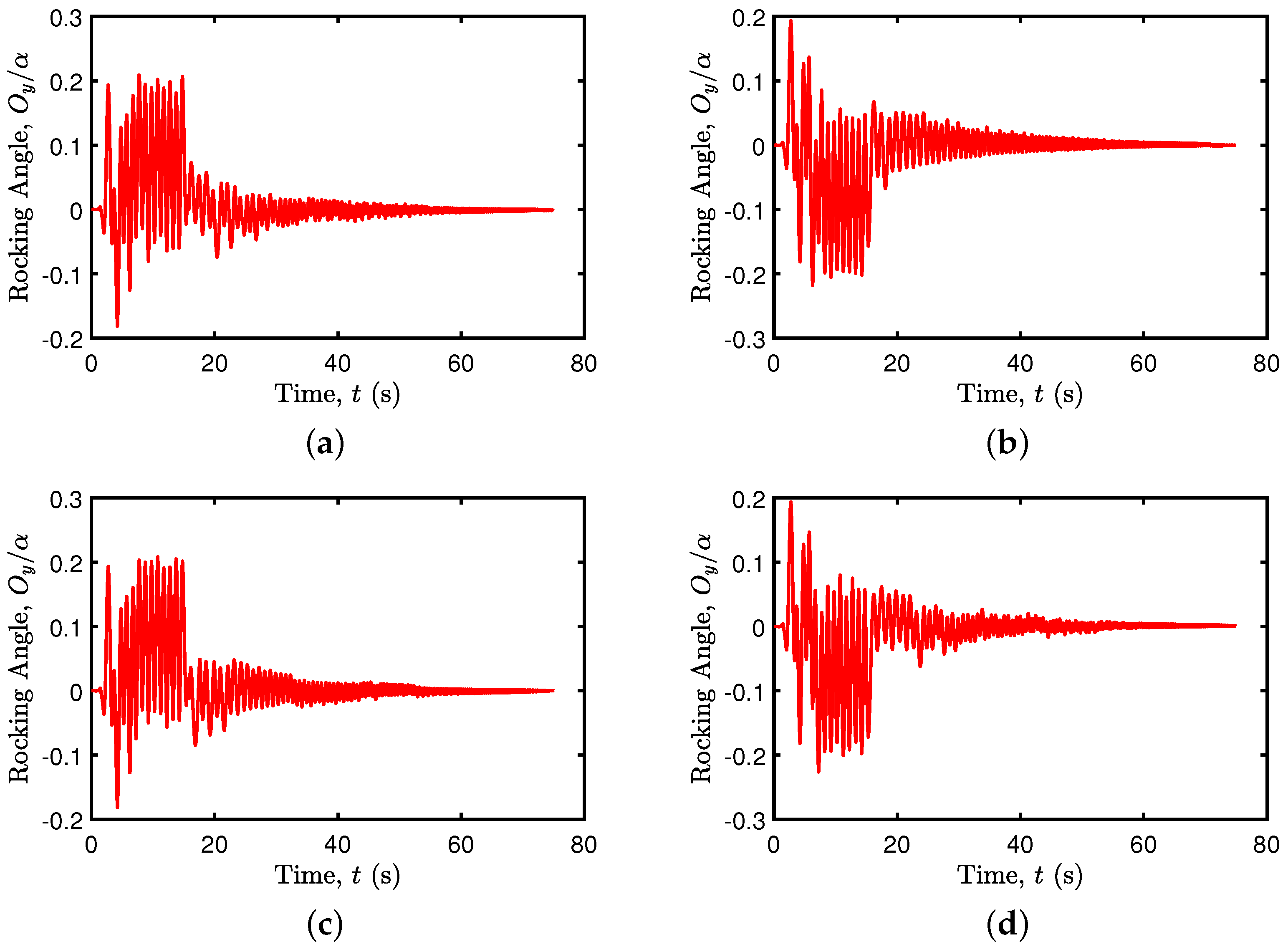
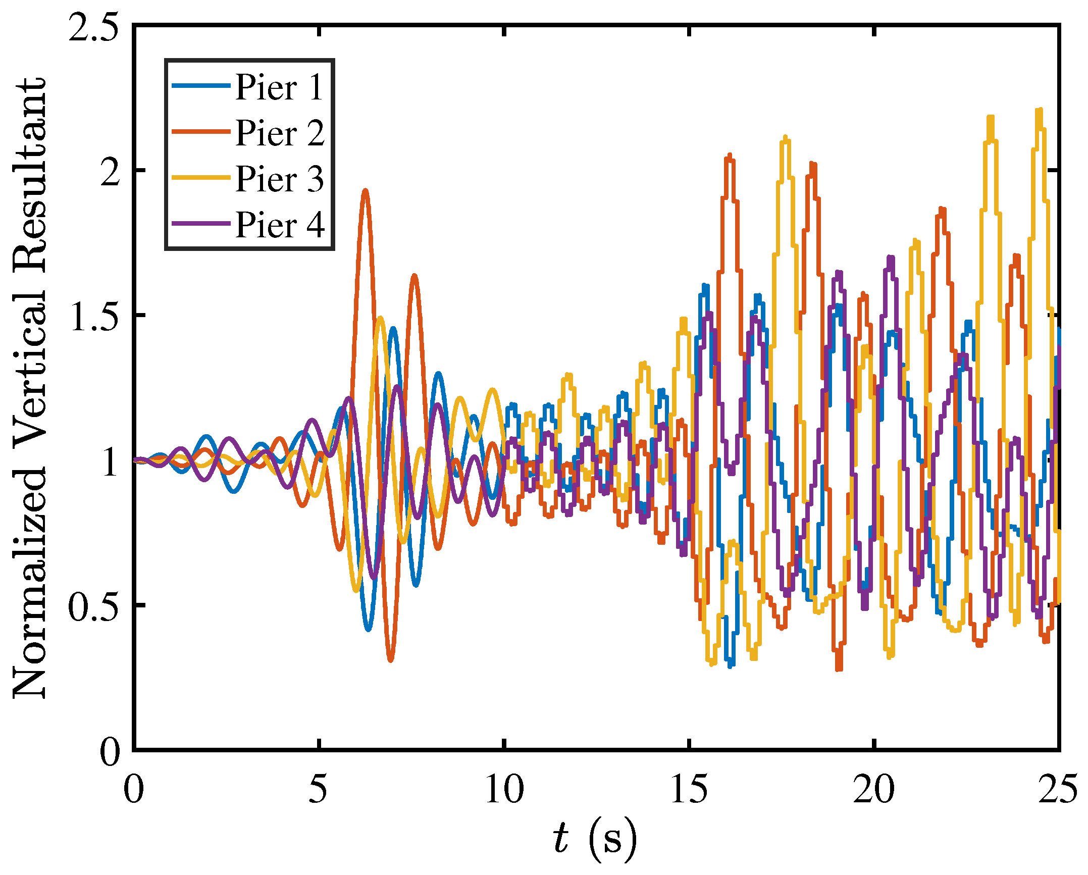
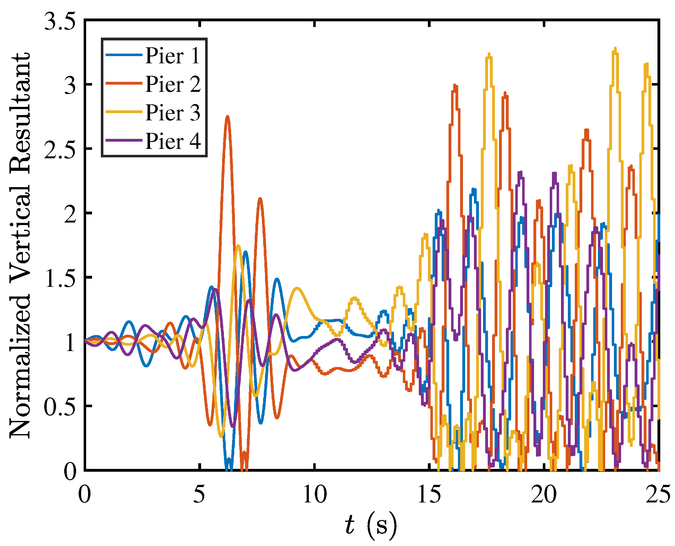
5.4. Rocking Isolation in Pier–Deck Systems under High-Intensity Excitation
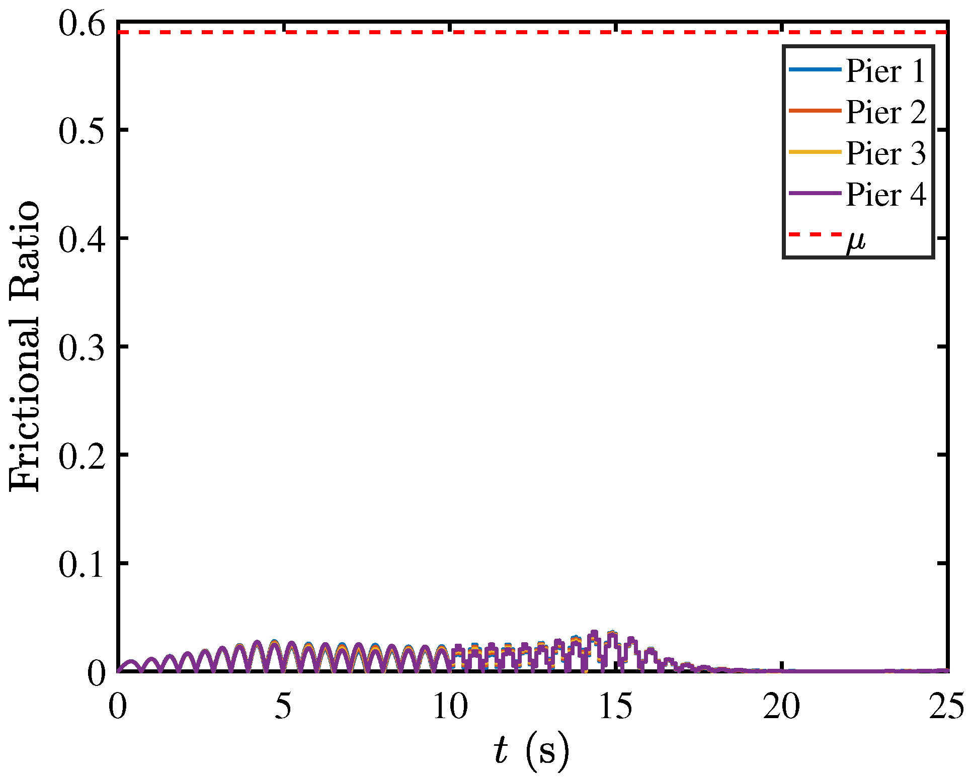
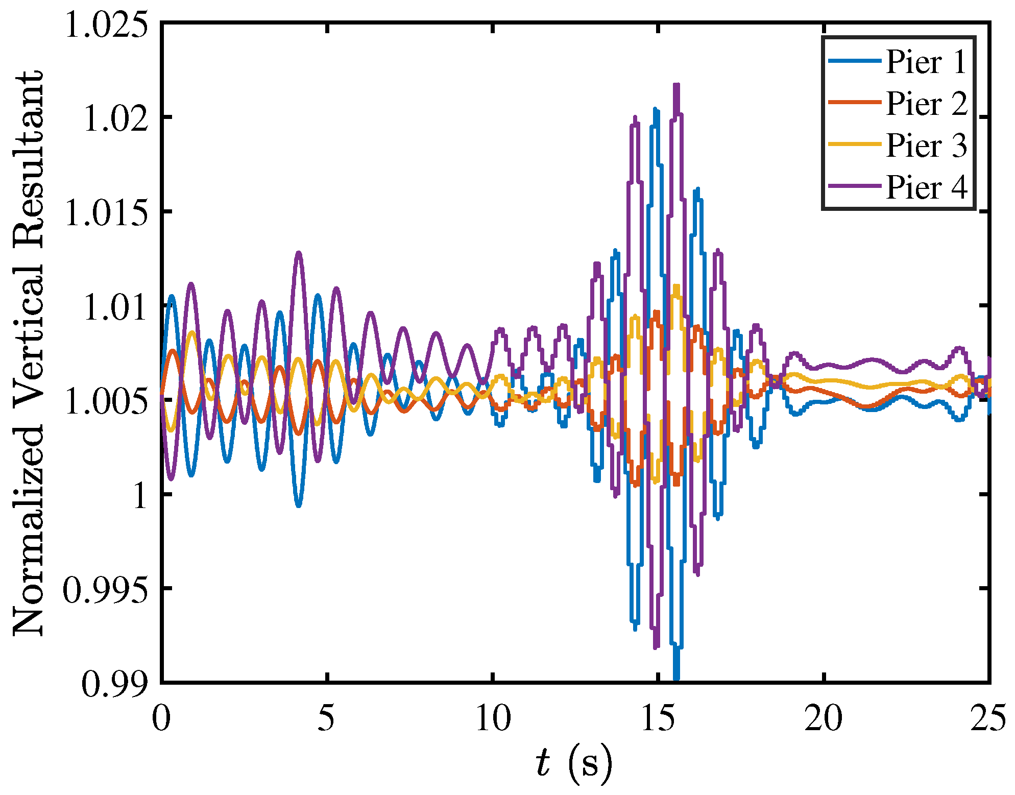
5.5. Contact Mechanics in Pier–Deck System under High-Intensity Excitation
6. Conclusions
Author Contributions
Funding
Data Availability Statement
Acknowledgments
Conflicts of Interest
References
- Mavroulis, S.; Argyropoulos, I.; Vassilakis, E.; Carydis, P.; Lekkas, E. Earthquake Environmental Effects and Building Properties Controlling Damage Caused by the 6 February 2023 Earthquakes in East Anatolia. Geosciences 2023, 13, 303. [Google Scholar] [CrossRef]
- Housner, G.W. The behavior of inverted pendulum structures during earthquakes. Bull. Seismol. Soc. Am. 1963, 53, 403–417. [Google Scholar] [CrossRef]
- Makris, N.; Roussos, Y. Rocking Response and Overturning of Equipment under Horizontal Pulse-Type Motions; Pacific Earthquake Engineering Research Center: Berkeley, CA, USA, 1998. [Google Scholar]
- Makris, N.; Roussos, Y. Rocking response of rigid blocks under near-source ground motions. Geotechnique 2000, 50, 243–262. [Google Scholar] [CrossRef]
- Makris, N.; Chang, S.P. Response of damped oscillators to cycloidal pulses. J. Eng. Mech. 2000, 126, 123–131. [Google Scholar] [CrossRef]
- Makris, N. A half-century of rocking isolation. Earthq. Struct. 2014, 7, 1187–1221. [Google Scholar] [CrossRef]
- Chatzis, M.; Smyth, A. Modeling of the 3D rocking problem. Int. J. Non-Linear Mech. 2012, 47, 85–98. [Google Scholar] [CrossRef]
- Mergos, P.E. Sustainable and resilient seismic design of reinforced concrete frames with rocking isolation on spread footings. Eng. Struct. 2023, 292, 116605. [Google Scholar] [CrossRef]
- Makris, N. The role of the rotational inertia on the seismic resistance of free-standing rocking columns and articulated frames. Bull. Seismol. Soc. Am. 2014, 104, 2226–2239. [Google Scholar] [CrossRef]
- Makris, N.; Aghagholizadeh, M. Effect of supplemental hysteretic and viscous damping on rocking response of free-standing columns. J. Eng. Mech. 2019, 145, 04019028. [Google Scholar] [CrossRef]
- Rele, R.; Balmukund, R.; Bhattacharya, S.; Cui, L.; Mitoulis, S.A. Application of controlled-rocking isolation with shape memory alloys for an overpass bridge. Soil Dyn. Earthq. Eng. 2021, 149, 106827. [Google Scholar] [CrossRef]
- Al-Aayedi, H.K.; Aldefae, A.H.; Shamkhi, M.S. Seismic performance of bridge piers. In Proceedings of the IOP Conference Series: Materials Science and Engineering, Assiut, Egypt, 11–12 February 2020; Volume 870, p. 012069. [Google Scholar]
- Thomaidis, I.M.; Camara, A.; Kappos, A.J. Dynamics and seismic performance of asymmetric rocking bridges. J. Eng. Mech. 2022, 148, 04022003. [Google Scholar] [CrossRef]
- Thomaidis, I.; Kappos, A.; Camara, A. Dynamics and seismic stability of planar symmetric rocking bridges. In Proceedings of the 2nd International Conference on Natural Hazards and Infrastructure, Chania, Greece, 23–26 June 2019. [Google Scholar]
- Skinner, R.; Beck, J.; Bycroft, G. A practical system for isolating structures from earthquake attack. Earthq. Eng. Struct. Dyn. 1974, 3, 297–309. [Google Scholar] [CrossRef]
- Solberg, K.; Mashiko, N.; Mander, J.; Dhakal, R. Performance of a damage-protected highway bridge pier subjected to bidirectional earthquake attack. J. Struct. Eng. 2009, 135, 469–478. [Google Scholar] [CrossRef]
- Astaneh-Asl, A.; Shen, J.H. Rocking behavior and retrofit of tall bridge piers. In Proceedings of the Structural Engineering in Natural Hazards Mitigation (ASCE), Irvine, CA, USA, 19–21 April 1993; pp. 121–126. [Google Scholar]
- Gajan, S.; Godagama, B. Seismic performance of bridge-deck-pier-type-structures with yielding columns supported by rocking foundations. J. Earthq. Eng. 2022, 26, 640–673. [Google Scholar] [CrossRef]
- Gajan, S.; Soundararajan, S.; Yang, M.; Akchurin, D. Effects of rocking coefficient and critical contact area ratio on the performance of rocking foundations from centrifuge and shake table experimental results. Soil Dyn. Earthq. Eng. 2021, 141, 106502. [Google Scholar] [CrossRef]
- Gajan, S. Application of machine learning algorithms to performance prediction of rocking shallow foundations during earthquake loading. Soil Dyn. Earthq. Eng. 2021, 151, 106965. [Google Scholar] [CrossRef]
- Deng, L.; Kutter, B.L.; Kunnath, S.K. Seismic design of rocking shallow foundations: Displacement-based methodology. J. Bridge Eng. 2014, 19, 04014043. [Google Scholar] [CrossRef]
- Kourkoulis, R.; Gelagoti, F.; Anastasopoulos, I. Rocking isolation of frames on isolated footings: Design insights and limitations. J. Earthq. Eng. 2012, 16, 374–400. [Google Scholar] [CrossRef]
- Gelagoti, F.; Kourkoulis, R.; Anastasopoulos, I.; Gazetas, G. Rocking isolation of low-rise frame structures founded on isolated footings. Earthq. Eng. Struct. Dyn. 2012, 41, 1177–1197. [Google Scholar] [CrossRef]
- Scattarreggia, N.; Galik, W.; Calvi, P.M.; Moratti, M.; Orgnoni, A.; Pinho, R. Analytical and numerical analysis of the torsional response of the multi-cell deck of a collapsed cable-stayed bridge. Eng. Struct. 2022, 265, 114412. [Google Scholar] [CrossRef]
- Scattarreggia, N.; Salomone, R.; Moratti, M.; Malomo, D.; Pinho, R.; Calvi, G.M. Collapse analysis of the multi-span reinforced concrete arch bridge of Caprigliola, Italy. Eng. Struct. 2022, 251, 113375. [Google Scholar] [CrossRef]
- Scattarreggia, N.; Malomo, D.; DeJong, M.J. A new Distinct Element meso-model for simulating the rocking-dominated seismic response of RC columns. Earthq. Eng. Struct. Dyn. 2023, 52, 828–838. [Google Scholar] [CrossRef]
- Galvez, F.; Sorrentino, L.; Dizhur, D.; Ingham, J.M. Seismic rocking simulation of unreinforced masonry parapets and façades using the discrete element method. Earthq. Eng. Struct. Dyn. 2022, 51, 1840–1856. [Google Scholar] [CrossRef]
- Anastasopoulos, I.; Loli, M.; Georgarakos, T.; Drosos, V. Shaking table testing of rocking—Isolated bridge pier on sand. J. Earthq. Eng. 2013, 17, 1–32. [Google Scholar] [CrossRef]
- Loli, M.; Knappett, J.A.; Brown, M.J.; Anastasopoulos, I.; Gazetas, G. Centrifuge modeling of rocking-isolated inelastic RC bridge piers. Earthq. Eng. Struct. Dyn. 2014, 43, 2341–2359. [Google Scholar] [CrossRef] [PubMed]
- Antonellis, G.; Gavras, A.G.; Panagiotou, M.; Kutter, B.L.; Guerrini, G.; Sander, A.C.; Fox, P.J. Shake table test of large-scale bridge columns supported on rocking shallow foundations. J. Geotech. Geoenviron. Eng. 2015, 141, 04015009. [Google Scholar] [CrossRef]
- Tsatsis, A.; Anastasopoulos, I. Performance of rocking systems on shallow improved sand: Shaking table testing. Front. Built Environ. 2015, 1, 9. [Google Scholar] [CrossRef]
- Liu, W.; Hutchinson, T.C.; Gavras, A.G.; Kutter, B.L.; Hakhamaneshi, M. Seismic behavior of frame-wall-rocking foundation systems. II: Dynamic test phase. J. Struct. Eng. 2015, 141, 04015060. [Google Scholar] [CrossRef]
- Madaschi, A.; Gajo, A.; Molinari, M.; Zonta, D. Characterization of the dynamic behavior of shallow foundations with full-scale dynamic tests. J. Geotech. Geoenviron. Eng. 2016, 142, 04016026. [Google Scholar] [CrossRef]
- Ko, K.W.; Ha, J.G.; Park, H.J.; Kim, D.S. Centrifuge modeling of improved design for rocking foundation using short piles. J. Geotech. Geoenviron. Eng. 2019, 145, 04019031. [Google Scholar] [CrossRef]
- Pelekis, I.; Madabhushi, G.S.; DeJong, M.J. Seismic performance of buildings with structural and foundation rocking in centrifuge testing. Earthq. Eng. Struct. Dyn. 2018, 47, 2390–2409. [Google Scholar] [CrossRef]
- Agalianos, A.; Psychari, A.; Vassiliou, M.F.; Stojadinovic, B.; Anastasopoulos, I. Comparative assessment of two rocking isolation techniques for a motorway overpass bridge. Front. Built Environ. 2017, 3, 47. [Google Scholar] [CrossRef]
- Makris, N. Seismic isolation: Early history. Earthq. Eng. Struct. Dyn. 2019, 48, 269–283. [Google Scholar] [CrossRef]
- Zhong, C.; Christopoulos, C. Shear-controlling rocking-isolation podium system for enhanced resilience of high-rise buildings. Earthq. Eng. Struct. Dyn. 2022, 51, 1363–1382. [Google Scholar] [CrossRef]
- Cundall, P.A.; Strack, O.D. A discrete numerical model for granular assemblies. Geotechnique 1979, 29, 47–65. [Google Scholar] [CrossRef]
- Galvez, F.; Sorrentino, L.; Dizhur, D.; Ingham, J.M. Using DEM to investigate boundary conditions for rocking URM facades subjected to earthquake Motion. J. Struct. Eng. 2021, 147, 04021191. [Google Scholar] [CrossRef]
- Sarhosis, V.; Lemos, J.; Bagi, K. Discrete Element Modeling. Numerical Modeling of Masonry and Historical Structures; Elsevier: Amsterdam, The Netherlands, 2019; pp. 469–501. [Google Scholar]
- Xu, N.; Zhang, J.; Tian, H.; Mei, G.; Ge, Q. Discrete element modeling of strata and surface movement induced by mining under open-pit final slope. Int. J. Rock Mech. Min. Sci. 2016, 88, 61–76. [Google Scholar] [CrossRef]
- Andrade, J.E.; Rosakis, A.J.; Conte, J.P.; Restrepo, J.I.; Gabuchian, V.; Harmon, J.M.; Rodriguez, A.; Nema, A.; Pedretti, A.R. A framework to assess the seismic performance of multiblock tower structures as gravity energy storage systems. J. Eng. Mech. 2023, 149, 04022085. [Google Scholar] [CrossRef]
- Peña, F.; Lourenço, P.B.; Campos-Costa, A. Experimental dynamic behavior of free-standing multi-block structures under seismic loadings. J. Earthq. Eng. 2008, 12, 953–979. [Google Scholar] [CrossRef]
- Peña, F.; Prieto, F.; Lourenço, P.B.; Campos Costa, A.; Lemos, J.V. On the dynamics of rocking motion of single rigid-block structures. Earthq. Eng. Struct. Dyn. 2007, 36, 2383–2399. [Google Scholar] [CrossRef]
- Zhang, J.; Makris, N. Rocking response of free-standing blocks under cycloidal pulses. J. Eng. Mech. 2001, 127, 473–483. [Google Scholar] [CrossRef]
- Shenton, H.W., III. Criteria for initiation of slide, rock, and slide-rock rigid-body modes. J. Eng. Mech. 1996, 122, 690–693. [Google Scholar] [CrossRef]
- Itasca Consulting Group. PFC3D (Particle Flow Code in Three Dimensions); Itasca Consulting Group: Minneapolis, MN, USA, 2019. [Google Scholar]
- Mindlin, R.D.; Deresiewicz, H. Elastic spheres in contact under varying oblique forces. J. Appl. Mech. 1953, 20, 327–344. [Google Scholar] [CrossRef]
- Ginsberg, J.H.; Genin, J. Statics and Dynamics; Wiley: Hoboken, NJ, USA, 1984. [Google Scholar]
- American Association of State Highway and Transportation Officials. AASHTO LRFD Bridge Design Specifications, 9th ed.; U.S. Customary Units, American Association of State Highway and Transportation Officials: Washington, DC, USA, 2020. [Google Scholar]
- Makris, N.; Vassiliou, M. Planar rocking response and stability analysis of an array of free-standing columns capped with a freely supported rigid beam. Earthq. Eng. Struct. Dyn. 2013, 42, 431–449. [Google Scholar] [CrossRef]


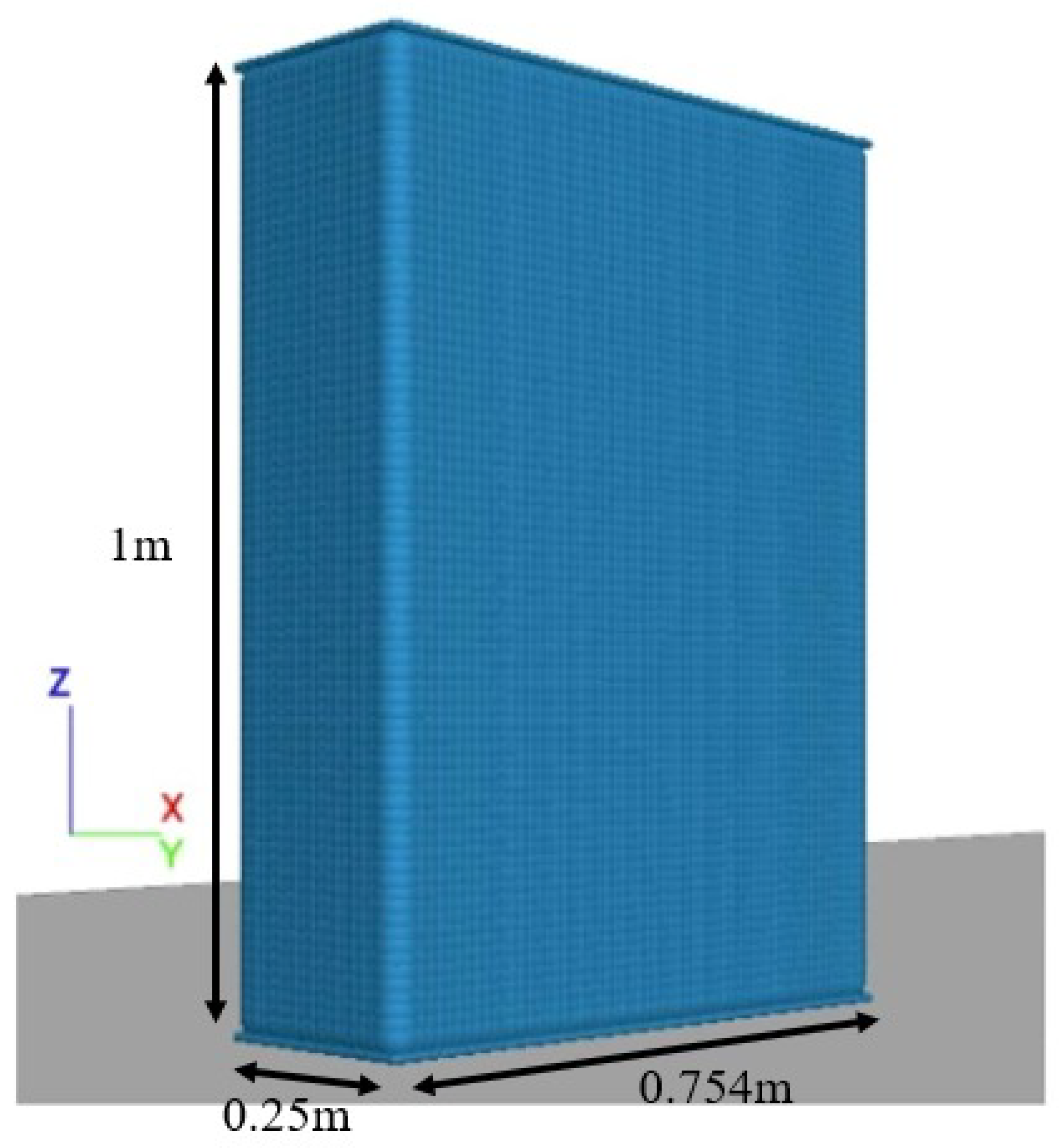
| Model Parameter | Pena’s Block | Base Wall |
|---|---|---|
| Width (m) | 0.25 | 1.0 |
| Height (m) | 1.0 | 0.25 |
| Thickness (m) | 0.754 | 0.75 |
| Mass (kg) | 503 | - |
| Inertia (kg.) | 37 | - |
| Parameter | Hertz Model |
|---|---|
| Poisson’s ratio, v | |
| Friction coefficient, | |
| Elastic modulus, E (Pa) | |
| Shear modulus, G (Pa) | |
| Normal viscous damping ratio, | |
| Shear viscous damping ratio, | |
| Density (kg/) | |
| Particle radius (m) | |
| Number of balls | 132,231 |
| Initial angular velocity (rad/s) | |
| Timestep (s) |
| Parameter | Hertz Model |
|---|---|
| Poisson’s ratio, | 0.16 |
| Friction coefficient, | 0.59 |
| Effective modulus (force/area), E (Pa) | |
| Shear modulus (stress), G (Pa) | |
| Normal viscous damping ratio, | 0.015 |
| Shear viscous damping ratio, | 0.015 |
| Density (kg/) | 2320 |
| Particle radius (m) | |
| Number of balls | 65,851 |
| Timestep (s) |
Disclaimer/Publisher’s Note: The statements, opinions and data contained in all publications are solely those of the individual author(s) and contributor(s) and not of MDPI and/or the editor(s). MDPI and/or the editor(s) disclaim responsibility for any injury to people or property resulting from any ideas, methods, instructions or products referred to in the content. |
© 2024 by the authors. Licensee MDPI, Basel, Switzerland. This article is an open access article distributed under the terms and conditions of the Creative Commons Attribution (CC BY) license (https://creativecommons.org/licenses/by/4.0/).
Share and Cite
Itiola, I.; El Shamy, U. A Microscale Framework for Seismic Stability Analysis of Bridge Pier Rocking Isolation Using the Discrete Element Method. Geotechnics 2024, 4, 742-772. https://doi.org/10.3390/geotechnics4030039
Itiola I, El Shamy U. A Microscale Framework for Seismic Stability Analysis of Bridge Pier Rocking Isolation Using the Discrete Element Method. Geotechnics. 2024; 4(3):742-772. https://doi.org/10.3390/geotechnics4030039
Chicago/Turabian StyleItiola, Idowu, and Usama El Shamy. 2024. "A Microscale Framework for Seismic Stability Analysis of Bridge Pier Rocking Isolation Using the Discrete Element Method" Geotechnics 4, no. 3: 742-772. https://doi.org/10.3390/geotechnics4030039