Abstract
Understanding the behavior of weak rock masses is important for predicting the stability of structures under different loading conditions. Traditional models such as the generalized Hoek–Brown and Coulomb weak plane are widely used; however, they often fail to capture the nonlinear and irreversible behavior of weak rock masses. This study offers a comprehensive overview of a critical analysis of constitutive models’ strengths and limitations for simulating weak rock masses. By comparing traditional and advanced novel approaches such as the strength degradation of rock (SDR) masses and continuous damage mechanics (CDM), this investigation shows that the new advanced methods significantly enhance the quality and accuracy of simulations. Moreover, SDR models address the limitations of classical plasticity models by incorporating nonlinear stress paths and irreversible stress changes, while CDM offers detailed insights into microstructural defect progression. These advancements allow for more accurate and practical predictions of long-term stability in geomechanical engineering tailored to specific requirements of each project.
1. Introduction
Understanding the mechanical behavior of rock masses, particularly weak rock masses, is critical for predicting geological and structural performance under various stress conditions. Accurately modeling the behavior of weak rock masses requires advanced simulation techniques that can accommodate the complex behavior and inherent physical characteristics of these materials.
Constitutive models play a critical role in simulating the behavior of weak rock masses. However, their development is fundamentally dependent on empirical data obtained through experimental methods. Traditional models, such as the generalized Hoek–Brown and Coulomb weak plane models, have been widely used to account for the anisotropy introduced by jointed weak rock masses and other discontinuities [1,2]. While these models provide foundational frameworks, they often fall short in capturing the nonlinear and irreversible behavior exhibited by weak rock masses under varying stress conditions. This limitation has led to the development of more sophisticated models, including hardening and softening models, that simulate the transition from peak to residual strength [3,4]. The accuracy and reliability of these advanced models are critically informed by test methods, such as triaxial compression tests, shear tests, and in situ load tests, which provide essential data for model calibration and validation. These experimental techniques ensure that the constitutive models are not only theoretical constructs but are also grounded in observed behavior of rock masses under real-world conditions.
In recent years, novel approaches like strength degradation of rock (SDR) masses models and continuous damage mechanics (CDM) have emerged. These models refine the accuracy of the simulation by incorporating nonlinear stress paths, structure degradation mechanisms, and the impact of accumulated plastic shear strain [5,6,7]. The SDR model, developed by Kalos et al. in 2017 [5], addresses limitations in traditional plasticity models and provides a framework for predicting long-term stability. CDM offers detailed insights into the progression of microstructural defects and their impact on material properties.
Controversies in the field arise from differing views on finding the most reliable approaches to simulate weak rock masses. Some researchers advocate for the use of empirical and practical data integration models, emphasizing the importance of the in-situ load test for accurate predictions [8,9,10,11]. Many scientists emphasize the importance of advanced constitutive models that incorporate statistical strength theory and damage mechanics, despite their computational complexity and the need for extensive calibration [12,13]. Others may point out that modeling scenarios where large deformations or significant material flow, complex geometries and boundary conditions, and the explicit representation of discontinuities, such as faults, joints, or fractures, are essential, numerical methods like finite element analysis (FEA) and discrete element modeling (DEM) are better suited to capture the behavior of discontinuous media. With the advent of machine learning models in recent years, one could also contemplate situations where these models would be trained to predict the overall behavior or performance of a rock mass (strength and deformation) where limited data are available, to detect anomalies based on real-time incoming data streams from sensors, and where the underlying physical processes are not well understood or difficult to model analytically, to potentially identify patterns and relationships in the data that traditional models do not easily capture.
The primary aim of this study is to provide a comprehensive overview and critical analysis of various constitutive models for simulating a weak rock mass. By comparing the traditional and novel approaches, this paper seeks to highlight the strengths and limitations of each method and offer recommendations for their applications in geomechanical engineering.
For the purposes of this study, the terms modeling and simulation are used interchangeably throughout the paper.
2. Materials and Methods
This study presents a comprehensive review of constitutive models employed in the simulation of weak rock mass behavior. We critically analyze current and historical methodologies for characterizing the deformation and failure mechanisms of weak rock masses under varying stress conditions. This analysis encompasses various approaches, including those based on elastoplastic, viscoplastic, and damage mechanics frameworks. Furthermore, we investigate the application of these models to diverse geological settings and loading scenarios, highlighting the strengths and limitations of each approach. This includes laboratory methods, computational methods and experimental field studies or any other novel approaches. Furthermore, a comparative analysis of these methodologies and their advantages, limitations, and sustainability are discussed.
2.1. Strength and Deformation Characterization Models
2.1.1. Generalized Hoek–Brown and Coulomb Weak Plane Models
These models adapt the traditional Hoek–Brown failure criterion (Equation (1)) and Coulomb’s law (Equation (2)) to account for anisotropy introduced by joints, bedding planes, and other discontinuity. Equation (1) incorporates several parameters, including , which is the major principal stress, is the minor principal stress, is the uniaxial compressive strength of the intact rock, is the Hoek–Brown constant for the rock masses, is a rock characteristic parameter, and is the empirical constant that accounts for the shape of the failure envelope. Equation (2) involves shear strength , effective cohesion , effective normal stress , and the effective angle of internal friction shown in . Unlike simpler elastic models, this approach accounts for directional dependence of the applicability of these models and was extended by using a set of weak planes, allowing for the simulation of anisotropic rock masses [2].
2.1.2. Softening and Hardening Models
This method simulates the weakening (softening) or strengthening (hardening) behavior of rock masses by using plasticity theories as they experience deformation. In this approach, the nonlinear transition from peak to residual strength is simulated, a feature that is captured by neither elastoplastic nor perfectly plastic models.
Hardening Models
Hardening defines how a material’s resistance and strength against deformation increases by plastic deformation. In other words, this phenomenon describes how the yield stress of a material changes with plastic deformation. The model is categorized into four parts: isotropic hardening, kinematic hardening, mixed hardening, and anisotropic hardening, illustrated below in depth.
Isotropic hardening assumes the material expands uniformly. In this regard, in isotropic hardening models, during the plastic deformation, the yield surface expands uniformly in the stress space shown in Equation (3), where is the current yield stress, is the initial yield stress, is the isotropic hardening modulus, and is the equivalent plastic strain [4].
Kinematic hardening is another type of hardening model that translates the yield surface in the stress space without changing its size or shape. Equation (4) demonstrates the translation of yield surface to stress space where is the back stress tensor, is the kinematic hardening modulus, and is the plastic strain tensor [1].
Additionally, the mix hardening model combines isotropic and kinematic hardening models to account for both expansion and translation of the yield surface and for both expansion and translation of the yield surface into stress space. Finally, the anisotropic hardening model is introduced, which can be described by various models depending on the structure of the material and the loading conditions [14].
Softening Models
Softening rules, on the other hand, refer to the reduction in material strength and stiffness after a peak stress has been reached, resulting in an increased tendency of failure. In this regard, softening is a critical concept in understanding a possible failure of the material. This concept is divided into three categories: strain softening, damage softening, and viscoplastic softening. Strain softening characterizes the initiation and propagation of cracks or other localized defects, while stress decreases by incremental strain after a material has been yielded and deformed plastically, as illustrated in Figure 1. This figure shows the stress–strain relationships for the rock samples tested, showcasing the critical points of hardening and softening during the loading process.
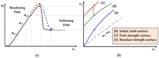
Figure 1.
Schematic diagram of the rock loading process: (a) stress–strain curve and (b) evolution of the loading path between characteristic yield surfaces [3].
The basic softening model consists of current stress , peak stress , as the softening modulus, current strain as , and as the current strain, shown in Equation (5) [6].
Additionally, damage softening involves progressive deterioration of material under load. Therefore, it is often modeled using damage mechanics. Damage softening models incorporate an accumulation of microstructural defects such as voids or microcracks, leading to macroscopic softening behavior.
The last definition is the viscoplastic models, which describe the rate-dependent behavior of materials that exhibit both viscous and plastic deformations, such as polymers or certain metals, at high temperatures.
Furthermore, the SDR method developed by Kalos et al. [5] illustrates this category by focusing on reduction strength due to accumulated strain, offering insights into long-term stability prediction.
Strain-Controlled Strength Degradation
In 2017, Kalos et al. developed the SDR, which represents an advancement in constitutive modeling by using a continuum mechanics incremental plasticity rate-independent constitutive model designed to account for structure and strength degradation due to the accumulation of plastic shear strain [5].
In [5], the SDR is built upon a generalized Hoek–Brown structure envelope in a stress environment characterized by a pressure-dependent curved failure envelope. This approach (SDR model) addresses limitations in the classical plasticity model that predict a large linear elastic domain up to the peak strength, perfect plastic strength without hardening or softening, and non-zero dilatancy at large strains.
The SDR model surpasses classical plasticity models by incorporating:
- (1)
- Nonlinear and irreversible stress paths.
- (2)
- Non-associated flow rule.
- (3)
- Structure degradation mechanism.
The nonlinear and irreversible stress path within the structure envelope (SE) simulates the nonlinear behavior of the weak rock mass up to the peak strength and under stress reversal conditions. In addition, it incorporates the non-associated flow rule in which the direction of plastic strain deformation does not match the direction of the stress vector causing the deformation. In this regard, this method was used to better control dilatancy especially at larger shear strains. The last method is the structure degradation mechanism to predict post-peak strain softening for brittle rock masses or strain hardening for ductile rock masses [5].
While the SDR model primarily is developed for weak rock masses, it can be used for simulating hard rocks by calibrating its parameters to reflect higher strength and stiffness characteristics typical for hard rock formations. This adaptability is centered on adjusting variables such as yield strength, stiffness reduction, and structural degradation coefficients that accurately simulate hard rock behavior [12]. Therefore, the SDR model is flexible for a range of rocks upon suitable parameter calibration and validation, making it more reliable for predictions.
Stress Path and Structure Envelope (SE)
The SDR model has differentiated between a “plastic” path that alters the material structure and a “non-plastic” path, which is nonlinear, but does not change the structure of the material. Moreover, the SE is defined as a stress space that includes plastic stresses on the envelope, leading to changes in structure. In contrast, non-plastic stress paths are considered inside the SE leading to nonlinear behavior without altering structure. The fundamental equation defining the structure envelope (SE) of the SDR model is crucial to understanding the constitutive model of rock mass simulation under different loading conditions, is defined in Equation (6). The model is a Hoek–Brown (HB) curve open surface stress in a stress hyperspace consisting of the isotropic axis and a five-dimensional deviatoric hyperplane. The key variables include the stress component along the x-axis , the Hoek–Brown constant for rock masses , cohesion , and the parameters , which adjust according to rock condition and typically represent a scaling factor that represents the yield criterion for different rock masses. Additionally, uniaxial compressive strength and F represent the failure condition function, which is equal to zero in the failure condition considered [5].
The SDR model allows for the gradual evolution of the structure parameters from their initial to final values with accumulated plastic shear strain, modeling strain hardening or softening depending on the evolution “friction angle” and the reduction in tensile strength with plastic strain, the evolution of which is “cohesion”. In this regard, the model includes hardening rules to control the evolution of structure variables with the incremental plastic strain. These rules can be applied to the hardening of the structure variable , which affects the shape of the axial curve and shear strain, as well as cohesion . When cohesion reaches its final value, then the material constant is equal to the accumulated plastic shear strain. Kalos et al. depicts the softening branches’ dependence on the plastic shear strain and demonstrates the model simulating the degradation of rock mass strength with increased plastic deformation, highlighting the importance of considering accumulated strain strength degradation due to accumulated plastic shear strain in material response [5]. In addition, the same paper shows how the structure variable can affect the shape of the shear strain and axial strain curve. Consequently, this effect demonstrates the model’s ability to account for different material behavior, including strain hardening and softening, by adjusting the variable.
Following this formula, the authors described other variables to capture the deformation of rock masses under different loading conditions. They described how the stiffness reduction variables evolve with the stress state inside the SE. The stiffness reduction variables include and , which control the nonlinearity and irreversibility of the material as a response to different loading conditions, and and represent the final or steady-state value of internal variables and after significant plastic deformation. and are initial values of internal variables representing the state of material before significant plastic deformation. controls the variables and and evolves as the material undergoes plastic deformation. is the reference stress function used to normalize the stress function in Equations (7) and (8).
This analysis explores the efficacy of a model in predicting stress behaviors within a structural element by contrasting its outputs under nonlinear and linear scenarios. It examines the model’s response to variations in stress related to volume and shape changes, termed volumetric and deviatoric stiffness, respectively, particularly under conditions where the material does not revert to its original form (non-plastic paths). Constants θ and ξ are employed within the model to maintain consistency in simulation parameters. This comparative approach demonstrates the model’s capability to accurately forecast material behaviors under varying stress conditions.
Hardening Rules
The model decomposes total strain into their plastic and elastic components to describe the relationship between total elastic and plastic strain increments, which is foundational for understanding how plastic deformation accumulates in rock mass. Equation (9) shows the basic of separation of the total strain increment () into its elastic () and plastic increment (), which can be decomposed into volumetric and deviatoric (shear) in Equation (10).
Flow Rule and Plastic Modulus
The model employs a flow rule to define plastic strain increment along with plastic paths by a potential tensor () with isotropic and deviatoric components , respectively), which gives directional information on the plastic strain increment () and scalar plastic multiplier that controls the magnitude of the plastic strain increment () shown in Equation (11). In addition, this model uses a non-associated flow rule for the volumetric components only, allowing the model to predict zero dilatancy at large accumulated shear strains, since dilatancy indicates a volume change in granular materials when they are subjected to shear deformation [9].
2.1.3. Elastoplastic Constitutive Models
Elastoplastic models are essential in understanding the behavior of rock masses that exhibit elastic or plastic deformations under load. This methodology is for analyzing compressible and incompressible materials or other materials that show different behaviors in tension and compression. The elastoplastic models constitute elastic, yield, and plastic criteria before showing hardening or softening behaviors, illustrated in Figure 2 and Figure 3, showing different elastoplastic nonlinear models. These figure illustrates the strain–stress behavior of material under loading, focusing on different modeling approaches for strain hardening and perfect plasticity. The figure depicts three possible paths that the material may follow depending on the constitutive model chosen: bilinear with perfect plasticity, bilinear with strain hardening, and multilinear strain hardening.
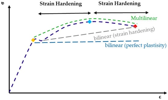
Figure 2.
Stress–strain curve for a ductile material [15].
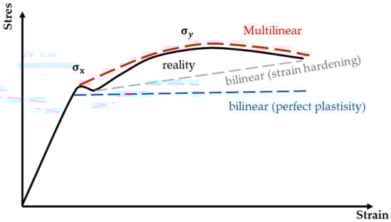
Figure 3.
Different elastoplastic models [16].
There are crucial criteria for developing a constitutive model for the onset of yielding and plastic deformation. There are several yield criteria for various materials and conditions, including the von Mises yield criterion, Tresca yield criterion, Mohr–Coulomb criterion, Drucker–Prager criterion, and Hill’s criterion.
The von Mises yield criterion in Equation (12), known as flow theory, suggests that yielding occurs when the energy distortion reaches a critical value that is the same as:
The Tresca yield criterion, known as the maximum shear stress criterion, proposes that yielding occurs when maximum shear stress in material reaches the maximum shear stress in simple tension tests. Equation (13) is an extended version of the von Mises yield criterion that includes other ductile materials besides metals:
where and are the principal stresses, the difference between them represents the maximum shear stress, and indicates the yield stress. The Tresca criteria is usually useful for materials that fail under shear stresses, such as brittle materials or metal at lower temperatures.
In addition, there is the Mohr–Coulomb yield criterion, which represents the 2D principal stress state as a series of straight lines, indicating the dependency on cohesion and internal friction angle (ϕ). This method in Equation (14)
The last one is the Drucker–Prager yield criterion, which is a 3D yield criterion in the form of a smooth cone around the hydrostatic axis approximating both von Mises and Mohr–Coulomb criteria, shown below in Equation (15). In this equation is the invariant of the stress tensor, defined as sum of the principal stresses. is the second invariant of the deviatoric stress tensor, which is a measure of the shear stress in the material. is often used in yield criteria like the Drucker–Prager or von Mises criterion, and is the constant that represents the yield criterion.
In general, von Mises and Drucker–Prager criteria are employed for 3D spaces creating a smooth surface around the pressure or hydrostatic axis. On the other hand, the Tresca criterion visualizes a hexagon in a deviatoric plane, indicating that yield can occur at a specific shear stress level. Moreover, the Mohr–Coulomb criterion is depicted through a 2D plot of normal stress versus shear stress, an indication of failure under combined stress conditions.
2.1.4. Ubiquitous-Joint Models
Ubiquitous-joint models are used to describe the mechanical behavior of rock masses that contain joints and faults, designed to account for weak (joints) of rock masses. These models predict the behavior of the rock mass material by incorporating their mechanical property matrices, like rock and joints. Additionally, the accounts for the anisotropic nature of rock masses and the mechanical response influenced by joint orientation and strength. It can predict failure along joints without the intact rock itself failing.
The equations for ubiquitous-joint models typically involve a combination of following components.
Strain–Stress Relationship
The general stress–strain relationship for rock mass can be expressed using the stress tensor , the stiffness matrix of the rock mass, which incorporates the mechanical properties of both the intact rock and joints , and the strain tensor [17], as illustrated in Equation below:
Joint Orientation and Strength
Anisotropy Consideration
Failure Criteria
Failure alongside the joints is often predicted using a criterion such as Mohr–Coulomb or Barton–Bandis, adapted to account for joint properties:
where is the shear stress along the joint, is the cohesion of the joint, is the cohesion of the joint, and is the friction angle of the joint [20].
Composite Yield Criterion
For cases where failure can occur in both the intact rock and along the joints, a composite yield criterion may be used:
where and represent yield functions for the intact rock and the joints, respectively [21].
Damage Evolution
Damage Mechanics Models
Damage mechanics models focus on the progressive deterioration of materials under different loading conditions. These models consider the effects of microstructural defects such as cracks, voids, and other inclusions that progressively deteriorate the material’s properties.
The damage variable includes a scalar or tensor, which represents the state of the damage in a material, typically ranging from 0 (undamaged material) to 1 (complete failure). There are some equations that encapsulate the core idea of the principle of continuous damage mechanics. Equation (21) represents damage as a reduction in material stiffness, where is the current modulus of the damaged material, and is the young modulus of undamaged material. Meanwhile, there is an effective stress concept in Equation (22), which adjusts the nominal stress () accounting for the presence of damage, where is the damage variable [22].
Another simplified model is the energy equivalence principle, which suggests that the work done on a damaged material is equivalent to the work that would be done on undamaged material, where and are all the strains in the damaged and equivalent undamaged material, respectively. This principle provides a basis for determining how damage affects a material’s stiffness and strength, serving as a foundation for formulating damage evolution laws:
Continuous Damage Mechanics
Continuous Damage Mechanics (CDM) involves a theoretical framework and empirical observations used to describe the damage and failure processes in jointed rock masses under triaxial loading conditions. This method evaluates the impact of stress states on rock structural damage to predict the failure of the material due to the evolution of microlevel defects, such as cracks, voids, and any inclusions that accumulate over time and stress states.
The damage evolution law is the other principle under continuous damage mechanics that describes how damage progresses toward failure under different loading conditions. This principle ensures predicting the lifetime of material and structures, as it describes how quickly damage progresses toward failure under different loading conditions. A generic formula is depicted where the rate of damage evolution is a function of the stress state and the current damage state [6]:
The thermodynamics of irreversible processes is another principle that CDM often relies on to formulate constitutive relations of damaged material by using the second law of thermodynamics and the concept of dissipative energy to model damage evolution. Indeed, the principle is that the damage mechanics models are thermodynamically consistent, allowing for the prediction of material behavior under complex loading and environmental conditions. The model relates the change in free energy of a system to the work done , and heat exchange , where is temperature and is the change in entropy [23]:
Continuous damage mechanics models damage within a continuum mechanics framework, considering the material as a continuous media despite microlevel cracks. The balance of momentum in continuum mechanics is expressed by the following equation, where σ is the stress tensor, is the body of the force vector, is the density, and is the acceleration vector [24].
Finally, the last principle under CDM is a generalized model showing damage evolution as a function of temperature , current damage , and strain , illustrating the coupling with thermal processes. Recognizing and modeling this interaction is critical for predicting material behavior in real-world conditions, especially in high-temperature applications or aggressive environments [25].
Indeed, CDM considers the progressive nature of damage, which can lead to eventual failure, which is a powerful tool to model and predict material behavior under stress.
Chen et al. [26] developed a constitutive model synthesizing Weibull statistical damage theory and fracture mechanics to analyze the behavior of jointed rock masses under triaxial compression.The foundational concept of the model is a geometric configuration of the joints within a rock mass, including spacing, orientation, and size, which are critical inputs that influence the initial damage estimation.
Furthermore, Chen et al. evaluated Equation (28) for the initial damage () done by joints before external pressure is applied, focusing on the importance of the rock’s initial condition When pressure is applied, the rock sustains additional damage, requiring further calculations to combine the initial damage with stress-induced damage. This illustrates how the rock’s condition evolves under pressure, incorporating joint and load-induced damage (Equation (29)). Additionally, Equation (30) integrates various damage components, including the progression from initial to total damage. The terms, and account for stress-induced damage normalized by joint-induced damage, while reflects initial damage normalized by stress-induced damage.
As a result, it can be seen in Equations (31) and (33) that the model’s parameters are related to joint geomaterial and the mechanical characteristic parameters, such as confining pressure, peak strength, and the elastic modulus of the jointed rock mass. The parameter reflects the average strength level of the rock mass, and a higher suggests a higher strength.
Additionally, the theory was put into practice to show that the model can predict what happens inside the rock with different joint setups under various pressures, demonstrating its ability to handle complex real-world conditions. Furthermore, according to Equation (30) and available data, the damage evolution curve with different joint sets was evaluated.
The model was validated through comparing its predictions with experimental data obtained from triaxial compression test conducted on jointed rock masses. The result suggested that the model can predict the failure mechanism in real world scenarios.
The key strength of the model is its ability to consider complex behavior of rock, including anisotropy and damage progression. However, the model’s validation was limited to two degrees of fracture and considered only two only two-dimensional stress. This may not fully capture rock behavior under various environmental conditions, such as different initial fracture levels or more complex stress environments. The model could benefit from incorporating empirical data and practical testing to improve its accuracy in predicting real-world scenarios.
2.1.5. In Situ Load-Testing Interpretation
This methodology aims to interpret the behavior of the rock directly by using the data from the load test performed directly on the rock masses. By doing so, it provides valuable insights into the properties of weak rock masse such ass stiffness and strength, which are crucial for safety analysis.
Several types of in situ tests for weak rock masses are commonly used to evaluate the mechanical properties of the rock in its natural environment.
Plate Load Test
The plate load test is an in-situ testing method used to determine the bearing capacity of the ground and likely settlement. This test is mostly used for designing foundations, especially when structures are going to be built on soil that is not perfectly rigid. This test involves loading a steel plate placed at the foundation level measuring the settlements corresponding to each load increment [10].
The data observed from this test are plotted in load-versus-settlement curves. These curves are analyzed to determine the ultimate bearing capacity of soil, the safe load-bearing capacity, and the modulus of the subgrade reaction, which is a measure of soil stiffness.
Pressure meter test
The pressure meter test (PMT) is an in situ geotechnical test used to measure ground deformation. It involves inserting a probe into the ground and inflating it to exert pressure on the surrounding soil or rock mass. The test measures the ground’s response to this pressure, thereby providing data on rock mass stiffness, strength, and in situ stress conditions [11].
Dilatometer Test
The dilatometer test (DMT) is an in-situ test to assess weak rock properties. This method inserts a flat dilatometer blade into the ground at the test depth. The blade has a flexible membrane on one side that can be expanded horizontally into the soil. Furthermore, by applying controlled pressure to the membrane and measuring the soil’s displacement or dilation, weak rock parameters such as elasticity, lateral earth pressure coefficient, and the stratigraphy profile can be determined. This information is crucial for predicting settlement, designing foundations, and other geotechnical purposes [25].
Flat Jack
The flat jack test is another in situ test involving the insertion of a thin hydraulic jack into a small precut slot in the tested material. Once inserted, the jack is slowly pressurized, causing controlled deformation. This test helps evaluate the stress state of rock masses without causing significant damage to them. The flat jack test setup is illustrated with the actuator system and concrete test blocks.
Goodman Jack Test
The Goodman jack test is widely used to measure the deformation modulus of rock masses in the field. This method involves using a device called a Goodman jack, which is inserted into a bore hole drilled into the rock while hydraulic pressure is applied to the jack, causing it to expand against the borehole walls. Consequently, the deformation of the rock in response to the pressure is measured, resulting in the calculation of the rock deformation modulus [27].
Asem et al. used the in-situ load test dataset to develop a model that could elucidate the behavior of a drilled shaft in a weak rock mass. The methodology involves creating two types of datasets to develop a model that can predict peak side resistance, tip resistance, and load transfer function for rock sockets in weak rocks, as well as a weak rock mass deformation predictive model. The model was validated by comparing predictions made against real-world observations from in situ loaded tests. However, due to limited data and lack of model documentation quality, the model’s effectiveness and applicability was not justified.
Various load tests were carried out to create a side resistance and base resistance database. The side resistance database provides information about peak side resistance, and stress–shear displacement for the sidewall directly through in situ instrumentation. The base side database focuses on load-transfer functions for shaft bases, properties of intact rock, properties of soft rock masses, base resistance, initial normal stiffness, and drilled shaft geometry. Hence, the methodology aims to provide a comprehensive database on load–displacement responses and rock mass properties to address previous studies’ limitations.
Furthermore, the database is employed to assess existing predictive models for axial resistance, and settlement of the rock foundations. This involves analyzing the model’s ability to consider the variability in rock properties and its impact on foundations reliability.
For design purposes, Young’s modulus was estimated from a linear regression analysis by [28,29] of results from an in-situ plate test, where is the unconfined compressive strength (UCS) of the rock, which represents the maximum and axial compressive stress that a rock specimen can withstand under no confinement. The existing predictive base model includes a basic rock mass estimation modulus from unconfined compressive strength in a linear model:
For empirical side resistance models, Rosenberg and Journeaux [30] are among the first ones to provide a model for estimating peak side resistance based on the unconfined compressive strength of the rock. However, they did not come up with a mathematical formula. In this regard, Kulhawy [31] found the best-fit equation for their method, which constitutes the peak side resistance , in situ confining pressure , and unconfined compressive strength :
Asem provided a summary of the existing base resistance formula taken from an in situ test database to compare his features and existing assumptions of Rowe and Armitage in Equation (35) [28], Zhang and Einstein in Equation (36), and Stark et al. [32] and Baghdady [33] in Equation (37) iincorporates which is a dimensionless correction factor that accounts for the effects of rock mass conditions such as presence of discontinuities, weathering, or other factors that reduce the rock strength.
Furthermore, the variation in available theories for base resistance () and comparison with measured fracture initiation pressure is shown in Figure 4, which helps illustrate the theoretical underpinnings against the measured data, aiming at the model’s effectiveness in predicting base resistance in weak rock masses [34].
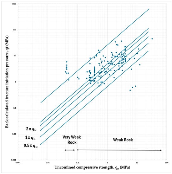
Figure 4.
Variation in available theories for base resistance ( and comparison with measured fracture initiation pressure ( (data from Asem and Gardoni [34]).
Besides base resistance, Carter and Kulhawy (1988) [30] presented a method for end resistance of foundation based on the Hoek–Brown failure criterion for jointed rock masses and developed foundation placed on the surface of rock masses (Figure 5):
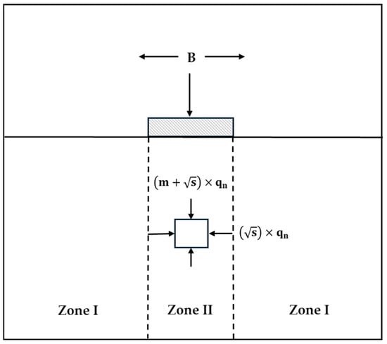
Figure 5.
Method of Carter and Kulhawy (1988) [30].
2.2. Variability and Heterogeneity Representation Models
2.2.1. Advanced Constitutive Modeling
This method involves developing complex mathematical models that demonstrate all behavior of weak rock masses under different loading conditions and identifies the failure mechanism and their effects in weak rock.
Amorosi et al. primarily focused on advanced constitutive modeling to develop an application of a hierarchical elastoplastic constitutive model specifically for structured soil and weak rock mass referred to as WR2 (weak rock type 2), which is a new versatile constitutive model for soft rocks and fine-grained soils based on the theory of single-surface elastoplasticity specifically designed for structured soil and weak rock mass [12]. This model is proposed by Boldini [35], who utilized a hyperplastic formulation for reversible responses and yield surface function to delimit the elastic domain based on stress invariants.
Hyperelastic formulations addresses the nonlinear relationship of elastic stiffness and its effective stress. However, a simplified linear version was adopted due to negligible stress sensitivity of the tuff under simulated conditions. Furthermore, the model utilized a yield surface function and hardening variables. To illustrate more, the yield function surface was utilized by a stress invariant, incorporating a meridian function based on mean effective pressure and deviatoric function influenced by the Lode angle. This function describes the cohesive and frictional plastic strain-induced degradation while considering state-controlled transition from dilatant to contractive responses. The model used volumetric and deviatoric plastic strain-induced structure degradation as part of an isotropic hardening function that governs the evolution of hardening variables based on plastic strain.
The model was validated by integrating a finite element code in Plaxis 3D and simulating drained triaxial tests. Consequently, the model was applied to analyze the stability of rock blocks on Ventotene Island. However, the limitations and future research directions highlight the need for further developments in the numerical approach and empirical evidence. Enhancing the model’s robustness through non-local FE formulations, expanding the experimental database for calibration, and establishing systematic in situ monitoring are crucial steps toward achieving a more accurate and reliable prediction of cliff instability processes.
2.2.2. Statistical Strength Theory Application
This approach applies to statistical methods to model the strength and failure of fractured rock masses by considering the randomness and variability inherent in rock properties and fracture distribution. Common distributions used in the SST (statistical strength approach) include normal or Gaussian distribution, log-normal distribution, and Weibull distribution. The choice of distribution depends on the nature of the property and the observed data. This method aims to provide a more realistic and reliable prediction of rock mass behavior under stress [36].
Chen et al. [37] presented a comprehensive investigation into development and verification of a novel constitutive model designed for fractured rock masses [38]. The model leverages continuous damage mechanics with statistical strength theory based on the Weibull distribution to describe the fracturing process in rock masses quantitatively. The authors introduced a new concept of the fracture degree that represents the extent of fracturing in rock masses and is crucial for assessing the behavior of the rock. Rock masses are divided into broken and unbroken parts. The fractures are randomly distributed, and hence the properties of broken part in each unbroken cube are randomly distributed. The fracture degree parameter ( is calculated by the statistical theory of randomness, where is the number of broken cubes (the fractures are caused by the loading process and do not contain initial fractures) and is the number of unbroken cubes showing the significance of the stress state:
Later, the authors linked the fracture probability to the stress state based on statistical strength theory. The key point of statistical damage constitutive modeling is to fit the analytical probability distribution to characterize the stress level of rock elements. In this regard, several empirical distributions have been used by the authors, such as Weibull distribution.
Oka et al. [13] presented a constitutive model to analyze the anisotropic behavior of soft sedimentary rocks [19]. In this paper, a comprehensive experimental study was carried out on the effects of sediments on soft rock through various orientations. A block of Tumoro stone was vertically sampled and cut into smaller specimens for triaxial compression tests. The concept of the model helps to investigate how the mechanical behavior of the sedimentary rock varies depending on the direction of the applied stress relative to the rock bedding. Therefore, the model incorporated parameters to account for the directional dependence of both the elastic and plastic behavior of the rock mass. They created an anisotropic elastoplastic model that incorporates strain softening and dilatancy effects that is dependent on the orientation of the loading condition for rock anisotropic material. In practical terms, a triaxial compressive test was conducted on rock specimens to provide data for calibration of the model parameters of the rock’s anisotropic characteristics. The advantage of this model is its ability to reproduce directional dependent behavior of soft sedimentary rocks. However, the complexity in determining model parametersintroduces limitations in replicating data, as it requires triaxial compression test of specimen samples in different directions. In addition, this model might be limited by its initial assumptions, as it assumes that the initial structural anisotropy is constant and does not change with loading.
2.3. Application of Machine Learning Methods
Machine learning (ML) is another method to simulate a weak rock mass that has gained significant interest in recent years. ML is a data-driven approach that complements traditional and advanced constitutive models by identifying complex patterns in large datasets, which are often difficult to capture using conventional models.
ML algorithms, including supervised learning, unsupervised learning and reinforcement learning, have been applied to predict the mechanical behavior of rock masses. These algorithms can be trained on vast amounts of data obtained from laboratory experiments, field studies, and numerical simulations. Once trained, these models can predict outcomes such as rock mass deformation, failure mechanisms, and stress–strain behavior under varying loading conditions [20].
There are several types of machine learning that have been utilized in constitutive modeling, including regression models, neural networks, support vector machines, decision trees and random forests, which will be illustrated below [39].
Regression Models
The continuous output of rock properties based on input features can be predicted by using linear or nonlinear regression models. These models are particularly useful for fitting constitutive models to experimental data.
Neural Networks
Artificial neural networks and deep learning are used for simulating rock masses with complex nonlinear relationships inherent in rock behavior. These models can account for high-dimensional interactions between different variables, providing more accurate predictions of rock mass responses.
Support Vector Machines
This type is used for classification tasks such as categorizing rock masses with different types of failure modes. This method is usually used where the data are not linearly separable, making it suitable for complex geotechnical datasets.
Decision Trees and Random Forests
Decision trees and random forests are useful to predict critical factors that influence rock mass behavior and predict outcomes based on hierarchical decision processes. These models are particularly useful in handling large datasets with numerous features.
Furthermore, machine learning models are not intended to replace traditional constitutive models, but rather to augment them. For example, ML models can be used to calibrate the parameters of traditional models more efficiently or to provide initial estimates where empirical data are sparse. Moreover, ML models can be integrated with numerical methods like finite element analysis (FEA) and discrete element modeling (DEM) to enhance the accuracy of simulations by providing better initial conditions or refining boundary conditions [36]. However, while machine learning shows great improvements in constitutive modeling, its application is still challenging. A key limitation is the need for extensive, high-quality datasets to train these models effectively. In geotechnical engineering, data are often limited, and acquiring datasets can be both logistically complex and expensive. Additionally, machine learning models often function as “black boxes,” delivering predictions without offering insight into the underlying physical mechanisms. This lack of transparency can be a notable disadvantage, especially in critical scenarios where understanding the mechanics behind predictions is just as crucial as the predictions themselves [37].
3. Results and Discussion
This review has explored a spectrum of constitutive methods and techniques designed to analyze the behavior of weak rock masses under different loading conditions and environments. Each method reviewed, from the fundamental generalized Hoek–Brown and Coulomb weak planes to sophisticated damage mechanics models, highlights the complexities and capabilities of accurately modeling geological properties. Constitutive models are indispensable tools for the analysis of weak rock masses due to their abilities as follows.
- Simulate time-dependent behavior: Weak rock masses often exhibit creep (gradual deformation under constant stress) and stress relaxation (decrease in stress under constant strain) over time. Constitutive models, particularly those incorporating viscoelastic or viscoplastic elements, effectively capture these time-dependent phenomena by considering the evolution of strain and stress as functions of time. This is crucial for predicting long-term deformations and assessing the stability of structures in weak rock over extended periods.
- Model behavior under dynamic loading: Weak rock masses can be subjected to dynamic loading conditions, such as seismic events or blasting, which induce rapid stress and strain changes. Constitutive models that incorporate rate-dependent material properties are essential for simulating the response of weak rock under these dynamic scenarios. By accounting for the influence of loading rate on rock behavior, these models enable engineers to assess the potential for dynamic failure and design appropriate mitigation measures.
- Assess long-term stability and failure mechanisms: The long-term stability of underground excavations or slopes in weak rock masses is a significant concern due to the potential for progressive failure mechanisms like strain softening, shear band formation, or time-dependent degradation of rock properties. Constitutive models, particularly CDM models that are capable of simulating damage or failure evolution, can predict these failure mechanisms and provide valuable insights into the potential for time-dependent deformations. Additionally, SDR models that incorporate stress paths and account for irreversible stress changes address a critical gap in the classical models. This information is crucial for designing safe and reliable engineering structures in weak rock environments.
- In addition to these capabilities, constitutive models can also be coupled with numerical analysis techniques, such as finite element or finite difference methods, to simulate the complex behavior of weak rock masses under various loading and environmental conditions. This allows engineers to perform comprehensive analyses and make informed decisions regarding the design, construction, and maintenance of structures in weak rock.
- Application to Diverse Geological Settings: This analysis extends to various geological settings and loading scenarios, which proves the adaptability and robustness of the advanced models, including SDR and CDM, which is particularly relevant for complex and anisotropic rock masses, where traditional models fall short.
Synthesizing theory and practice
The integration of theoretical models and practical insights provided by in situ load-testing interpretations forms a cornerstone of geotechnical engineering. Load-testing techniques provide crucial empirical data that can be used to calibrate and validate theoretical predictions. In situ tests like the plate load test, pressure meter test, and dilatometer test offer direct measurements of mechanical properties such as stiffness and strength in their natural environment, which is essential for accurate safety analysis and model validation. These models can ensure the reliability of constitutive models to predict the performance of weak rock mass under different loading conditions. Models like the generalized Hoek–Brown framework are crucial for anticipating failure surfaces and sustainability under stress. However, the real-world application of these models creates a gap between theoretical predictions and observed outcomes, primarily due to simplifications of model assumptions and inherent variability in geological properties.
On the other hand, advanced models that incorporate the hardening and softening behavior of the material address some of these issues by enhancing the assumptions of the models and closely simulating the actual response of rock mass to deformation. These models are crucially applicable in fields involving cyclic loading and long-term stability and provide a dynamic perspective that static models cannot manage. Nonetheless, determining the models’ parameters is still challenging, where discrepancies in material behavior under laboratory conditions and field conditions can lead to significant prediction errors.
Statistical Methods in Constitutive Modeling
Statistical methods serve as a strong tool to simulate the uncertainty and variability inherent in rock mass properties by the availability and quality of input data. By incorporating statistical theories into the constitutive model, probabilistic assessment of rock behavior will be possible. This method is applicable when empirical data are sparse and dealing with complex geological settings. For instance, the Weibull distribution has proven effective in modeling the strength of rock materials under stress. The reason that the Weibull distribution is preferred is that it is flexible and can assume various shapes depending on its parameters. The shape parameter (beta) controls the distribution shape, making it capable of modeling different failure behaviors, while the scale parameters η adjusts the distribution to fit the scale of the data, ensuring a more precise fit to observed data. The Weibull distribution effectively describes the distribution of flaws or microcracks within rock mass, as well as the scale effect, which is critical in understanding the overall strength of a material. Compared to traditional methods such as normal and log-normal distributions, the Weibull distribution captures the skewness and kurtosis present in the strength of weak rock masses due to its flexibility and adaptability.
Limitations and Challenges
The principal limitation in constitutive modeling of weak rock masses lies in the imprecise characterization of material properties that are inherently non-uniform and anisotropic. Despite all advances in in situ load-testing techniques, obtaining reliable data that reflect the complex interplay in mechanical behavior of rock masses remains challenging. In addition, the scale effect, where the behavior of rock masses is observed at different scales (e.g., microscale, mesoscale, and macroscale) does not linearly match the scale at the field level, which poses another significant barrier in reliably predicting rock behavior in the long term. Therefore, having a scaling law and using dimensionless parameters can address obstacles between small-scale experiments and large-scale field conditions.
Damage mechanics and continuous damage mechanics (CDM) have successfully simulated the initiation and evolution of microscale damage within rock masses. However, translating this microscale damage to macroscale behavior without oversimplification and calibration is a sophisticated process in engineering process.
Statistical methods require comprehensive and representative datasets that accurately reflect in situ test conditions, which remain challenging due to logistical, financial, and technical barriers. Moreover, the simplifications required to make these models computationally feasible results in the loss of critical detail and accuracy, particularly concerning microscale interactions within rock masses.
Numerical models, including finite element analysis (FEA) and discrete element modeling (DEM), along with machine learning (ML), have their own set of limitations. All three methods are dependent on significant computational resources, particularly for large-scale or highly detailed simulations, where high-performance computing environments are necessary for timely and accurate results. Furthermore, representing the heterogeneity and discontinuous nature of rock mass is challenging, since FEA struggles with mesh quality, DEM with realistic particle shape interaction, and ML with capturing variability in the data. Moreover, model calibration is essential for accurate simulations, which remains challenging with these methods due to their complexity. FEA and DEM involve tuning material properties and interaction parameters, while ML involves training models with sufficient and representative data. Therefore, using these models requires substantial expertise and experience, along with confidence in the availability of a considerable amount of high-quality data.
A common challenge across various rock mass constitutive modeling techniques is the accurate characterization of heterogeneous and anisotropic materials, as well as the consideration of scale effects. These factors pose significant obstacles to the successful application of these models. Additionally, validating model predictions against field data and laboratory results remains a crucial yet often challenging task.
Application in Geotechnical Engineering and Case Studies
The SDR and CDM models discussed in this study have been applied in various geotechnical engineering to predict the behavior of weak rock masses under different loading conditions. For instance, the SDR model has been implemented in the Abaqus finite element code Simulia and applied in a case study involving plain strain 2D excavation of a cylindrical cavity. This application highlighted the model’s ability to account for nonlinear stress paths, plastic strain increments, and the gradual evolution of structural variables [37]
Furthermore, the CDM model has been utilized in projects requiring detailed predation of damage processes, such as stability analysis of slopes and underground excavations. Engineers were able to dynamically update predictions and enact timely mitigation measures by integrating real-time data from sensors.
4. Conclusions
This review provides a comprehensive analysis of constitutive models used to simulate the behavior of weak rock masses, encompassing both traditional and advanced methodologies. It begins with evaluating foundational models like generalized Hoek–Brown and Coulomb weak plane models, which have been instrumental in understanding the anisotropic behavior of rock masses, highlighting their foundational role in understanding rock mass behavior. However, it also underscores the limitation of these traditional approaches, particularly in capturing nonlinear and irreversible behaviors under complex loading conditions.
The review also delves into more advanced models such as hardening and softening models, which provide more insight into the transition from peak to residual strength in weak rock masses. Indeed, these models are particularly useful in scenarios involving complex deformation patterns, where traditional elastoplastic models fall short.
Furthermore, the paper evaluates novel approaches such as strength degradation of rock masses (SDR) and continuous damage mechanics (CDM), which represent significant advancements in modeling rock mass behavior. These models enhance weak rock mass simulation approaches by improving the accuracy of simulations through incorporating nonlinear stress paths and microstructural damage progression, and are also valuable tools for long-term stability predictions in geomechanical engineering.
Additionally, the integration of empirical and practical data through in situ testing methods such as the plate load test and pressure meter test is discussed as a critical component for validating and calibrating these models. This integration ensures that the theoretical constructs are grounded in real-world observations, thereby improving the reliability of predictions.
In conclusion, this study emphasizes the importance of selecting the appropriate constitutive model based on the specific characteristics of the geological setting and demands of the engineering project. While advanced models like SDR and CDM offer unparalleled detail and accuracy, traditional models still hold value in certain contexts. This study advocates a balanced approach, where the choice of model is influenced by the specific requirements of each project to maintain theoretical rigor and practical applicability. In this regard, future research should be conducted to continue to explore integration of these models with emerging technologies such as machine learning to further enhance predictive capabilities and adapt to evolving challenges in this field.
Author Contributions
A.A. conducted the literature review and wrote the initial draft of the manuscript. M.M. revised and edited the manuscript. All authors have read and agreed to the published version of the manuscript.
Funding
There was no external funding provided to support this review paper and writing process. Therefore, there is no funding source or number to report.
Data Availability Statement
This is a review paper, and no new data were generated or analyzed in this study. Therefore, data availability is not applicable.
Conflicts of Interest
The authors declare no conflicts of interest.
References
- Chaboche, J.L. Constitutive equations for cyclic plasticity and cyclic viscoplasticity. Int. J. Plast. 1989, 5, 247–302. [Google Scholar] [CrossRef]
- Hoek, E.; Carranza-Torres, C.; Corkum, B. Hoek-Brown failure criterion—2002 edition. In Proceedings of the NARMS-TAC Conference, Toronto, ON, Canada, 2002; Volume 1, pp. 267–273. Available online: https://geotechpedia.com/Publication/Show/1215/HOEK-BROWN-FAILURE-CRITERION--2002-EDITION (accessed on 2 September 2024).
- Xiao, Y.; Qiao, Y.; He, M.; Li, H.; Cheng, T.; Tang, J. A unified strain-hardening and strain-softening elasto-plastic constitutive model for intact rocks. Comput. Geotech. 2022, 148, 104772. [Google Scholar] [CrossRef]
- Lemaitre, J.; Chaboche, J.L. Mechanics of Solid Materials; Cambridge University Press: Cambridge, UK, 1990. [Google Scholar] [CrossRef]
- Kalos, A.; Kavvadas, M. A Constitutive Model for Strain-Controlled Strength Degradation of Rockmasses (SDR). Rock Mech. Rock Eng. 2017, 50, 2973–2984. [Google Scholar] [CrossRef]
- Lemaitre, J. A Course on Damage Mechanics; Springer: Berlin/Heidelberg, Germany, 1996. [Google Scholar] [CrossRef]
- JianPing, Y.; WeiZhong, C.; DianSen, Y.; JingQiang, Y. Numerical determination of strength and deformability of fractured rock mass by FEM modeling. Comput. Geotech. 2015, 64, 20–31. [Google Scholar] [CrossRef]
- Pouliquen, O. Granular Media: Between Fluid and Solid; Cambridge University Press: Cambridge, UK, 2013. [Google Scholar] [CrossRef]
- Shahverdiloo, M.R.; Zare, S. A New Correlation to Predict Rock Mass Deformability Modulus Considering Loading Level of Dilatometer Tests. Geotech. Geol. Eng. 2021, 39, 5517–5528. [Google Scholar] [CrossRef]
- Mortazavi, A. An Investigation of the Mechanisms Involved in Plate Load Testing in Rock. Appl. Sci. 2021, 11, 2720. [Google Scholar] [CrossRef]
- Tang, Z. Theoretical and Experimental Development and Application of Pressuremeter Test (PMT) with Case Study of Victorian Brown Coal Open-Pit Mining. Ph.D. Dissertation, The University of Melbourne, Melbourne, Australia, 2012. [Google Scholar]
- Amorosi, A.; Rollo, F.; Gagliardini, L. The Analysis of Weak Rock Block Behaviour by an Advanced Constitutive Model. In Geotechnical Research for Land Protection and Development; Calvetti, F., Cotecchia, F., Galli, A., Jommi, C., Eds.; Springer: Cham, Switzerland, 2020; Volume 40, pp. 611–620. [Google Scholar] [CrossRef]
- Oka, F.; Kimoto, S.; Kobayashi, H.; Adachi, T. Anisotropic Behavior of Soft Sedimentary Rock and A Constitutive Model. Soils Found. 2002, 42, 59–70. [Google Scholar] [CrossRef]
- Llt, J. Plastic Behavior and Stretchability of Sheet Metals. Part I: A Yield Function for Orthotropic Sheets Under Plane Stress Conditions. Int. J. Mech. Sci. 1989, 31, 197–209. [Google Scholar]
- Zych, B. Analyzing a Stress-Strain Curve. J. Eng. Mech. 2019, 145, 04019051–1-8. [Google Scholar] [CrossRef]
- Belmouden, Y.; Lestuzzi, P. An Equivalent Frame Model for Seismic Analysis of Masonry and Reinforced Concrete Buildings. Constr. Build. Mater. 2009, 23, 40–53. [Google Scholar] [CrossRef]
- Gong, B.; Tang, C.; Wang, S.; Bai, H.; Li, Y. Simulation of the nonlinear mechanical behaviors of jointed rock masses based on the improved discontinuous deformation and displacement method. Int. J. Rock Mech. Min. Sci. 2019, 122, 104076. [Google Scholar] [CrossRef]
- Zhou, X.; Tang, C.A.; Li, W. Modeling the mechanical behavior of jointed rock masses with the synthetic rock mass approach. Eng. Geol. 2018, 110, 136–148. [Google Scholar] [CrossRef]
- Sadeghi, H.; Kiani, M.; Sadeghi, M.; Jafarzadeh, F. Geotechnical characterization and collapsibility of a natural dispersive loess. Eng. Geol. 2019, 250, 89–100. [Google Scholar] [CrossRef]
- Zhao, L.; Yu, C.; Cheng, X.; Zuo, S.; Jiao, K. A method for seismic stability analysis of jointed rock slopes using Barton-Bandis failure criterion. Int. J. Rock Mech. Min. Sci. 2020, 136, 104487. [Google Scholar] [CrossRef]
- Zhang, Q.; Quan, X.-W.; Wang, H.-Y.; Jiang, B.-S.; Liu, R.-C. A numerical solution of a circular tunnel in a confining pressure-dependent strain-softening rock mass. Comput. Geotech. 2020, 121, 103473. [Google Scholar] [CrossRef]
- Kachanov, L.M. Introduction to Continuum Damage Mechanics; Mechanics of Elastic Stability; Springer: Dordrecht, The Netherlands, 1986; Volume 10. [Google Scholar] [CrossRef]
- Selvadurai, A.P.S.; Suvorov, A.P. Thermo-Poroelasticity and Geomechanics, 1st ed.; Cambridge University Press: Cambridge, UK, 2016. [Google Scholar] [CrossRef]
- Zhang, H.; Qin, X.; Chen, M.; Yang, G.; Lu, Y. A Damage Constitutive Model for a Jointed Rock Mass under Triaxial Compression. Int. J. Geomech. 2023, 23, 04023059. [Google Scholar] [CrossRef]
- Zalesky, M.; Böhler, C.; Burger, U.; John, M. Dilatometer Tests in Deep Boreholes in Investigation for Brenner Base Tunnel. In Underground Space—The 4th Dimension of Metropolises; Hrdina, I., Ed.; Taylor & Francis: Abingdon, UK, 2007. [Google Scholar] [CrossRef]
- Chen, X.; Gao, W.; He, T.; Ge, S.; Ma, P.; Zhou, C. Study on Constitutive Model of Fractured Rock Masses by Using Statistical Strength Theory. Math. Methods Appl. Sci. 2023, 43, 2458–2470. [Google Scholar] [CrossRef]
- Hou, R.; Zhang, K.; Sun, K.; Gamage, R.P. Discussions on Correction of Goodman Jack Test. Geotech. Test. J. 2017, 40, 199–209. [Google Scholar] [CrossRef]
- Rowe, R.K.; Armitage, H.H. A Design Method for Drilled Piers in Soft Rock. Can. Geotech. J. 1987, 24, 126–142. [Google Scholar] [CrossRef]
- Asem, P. Axial Behavior of Drilled Shafts in Soft Rock. Ph.D. Dissertation, University of Illinois at Urbana-Champaign, Champaign, IL, USA, 2018. [Google Scholar]
- Rosenberg, P.; Journeaux, N.L. Friction and End Bearing Tests on Bedrock for High Capacity Socket Design. Can. Geotech. J. 1976, 13, 324–333. [Google Scholar] [CrossRef]
- Carter, J.; Kulhawy, F.H. Analysis and Design of Drilled Shaft; Cornell University: Ithaca, NY, USA, 1999. [Google Scholar]
- Stark, T.D.; Long, J.H.; Asem, P. Improvement for Determining the Axial Capacity of Drilled Shafts in Shale in Illinois; Geotechnical Research Report; Illinois Center for Transportation: Rantoul, IL, USA, 2013. [Google Scholar]
- Baghdady, A.K. Axial Behavior of Drilled Shafts Socketed into Weak Pennsylvanian Shales. Ph.D. Dissertation, University of Illinois at Urbana-Champaign, Champaign, IL, USA, 2018. [Google Scholar]
- Asem, P.; Gardoni, P. On the Use and Interpretation of In Situ Load Tests in Weak Rock Masses. Rock Mech. Rock Eng. 2021, 54, 3663–3700. [Google Scholar] [CrossRef]
- Boldini, D.; Palmieri, F.; Amorosi, A. A New Versatile Constitutive Law for Modelling the Monotonic Response of Soft Rocks and Structured Fine-Grained Soils. Numer. Anal. Methods Geomech. 2019, 43, 2383–2406. [Google Scholar] [CrossRef]
- Zhou, H.; Zhang, J.; Li, C. Artificial Neural Networks and Support Vector Machines for Predicting Rock Properties. Eng. Geol. 2018, 239, 34–46. [Google Scholar] [CrossRef]
- Chen, X.; Liu, Y.; Wang, T. Integration of Machine Learning with Traditional Geomechanical Models for Enhanced Prediction Accuracy. Int. J. Rock Mech. Min. Sci. 2019, 123, 104092. [Google Scholar] [CrossRef]
- Zhang, D.; Zhou, P.; Wang, L. Challenges in Applying Machine Learning to Geotechnical Engineering: A Review. Comput. Geotech. 2018, 95, 103–114. [Google Scholar] [CrossRef]
- Ma, J.; He, P.; Yang, W. Application of Machine Learning Techniques in Geotechnical Engineering: Recent Developments. J. Rock Mech. Geotech. Eng. 2020, 43–57. [Google Scholar] [CrossRef]
Disclaimer/Publisher’s Note: The statements, opinions and data contained in all publications are solely those of the individual author(s) and contributor(s) and not of MDPI and/or the editor(s). MDPI and/or the editor(s) disclaim responsibility for any injury to people or property resulting from any ideas, methods, instructions or products referred to in the content. |
© 2024 by the authors. Licensee MDPI, Basel, Switzerland. This article is an open access article distributed under the terms and conditions of the Creative Commons Attribution (CC BY) license (https://creativecommons.org/licenses/by/4.0/).