
The Theories of Rubber Elasticity and the Goodness of Their Constitutive Stress–Strain Equations


Abstract
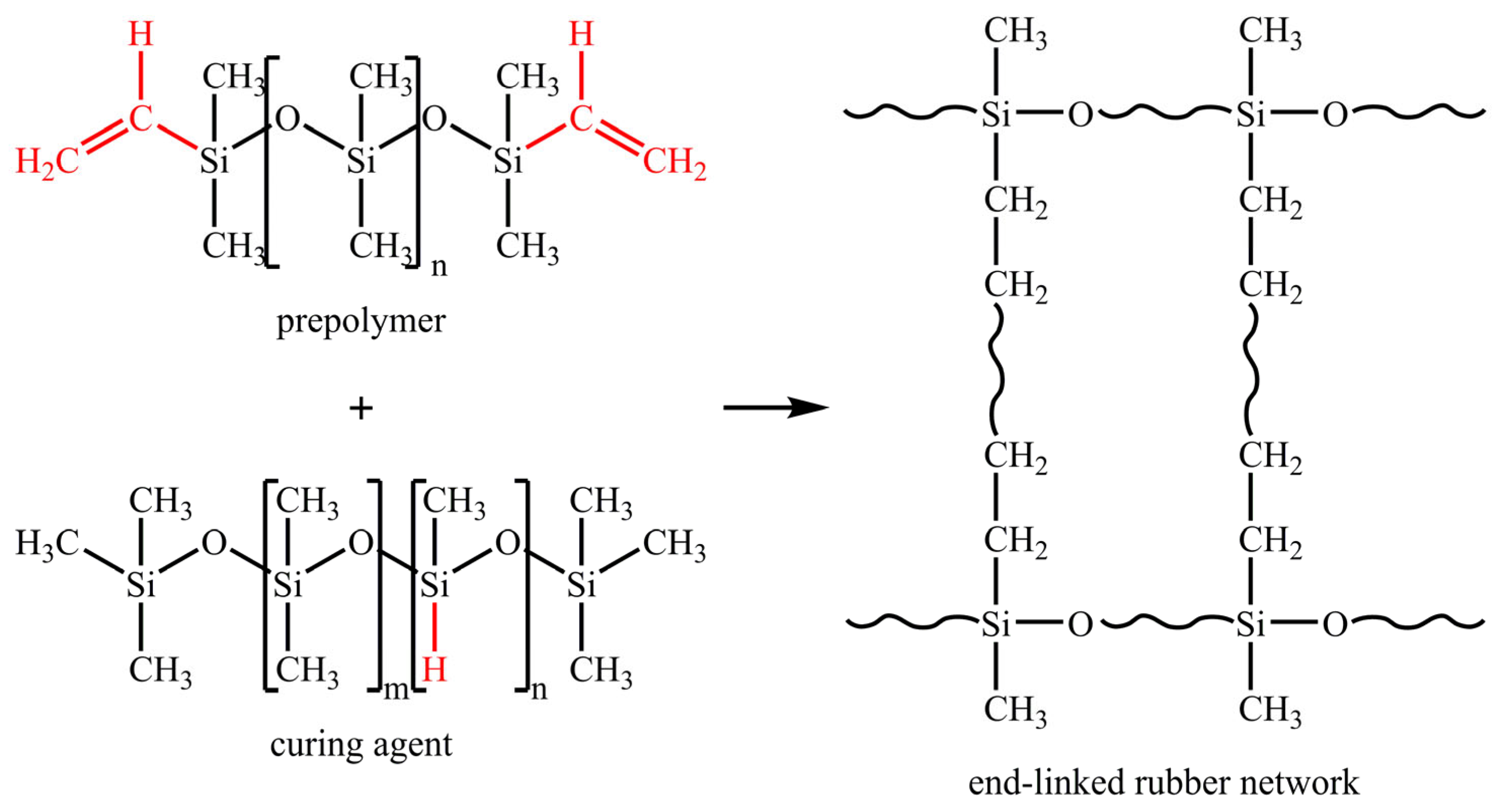
:1. Introduction
2. Experimental Method
3. Molecular and Phenomenological Models
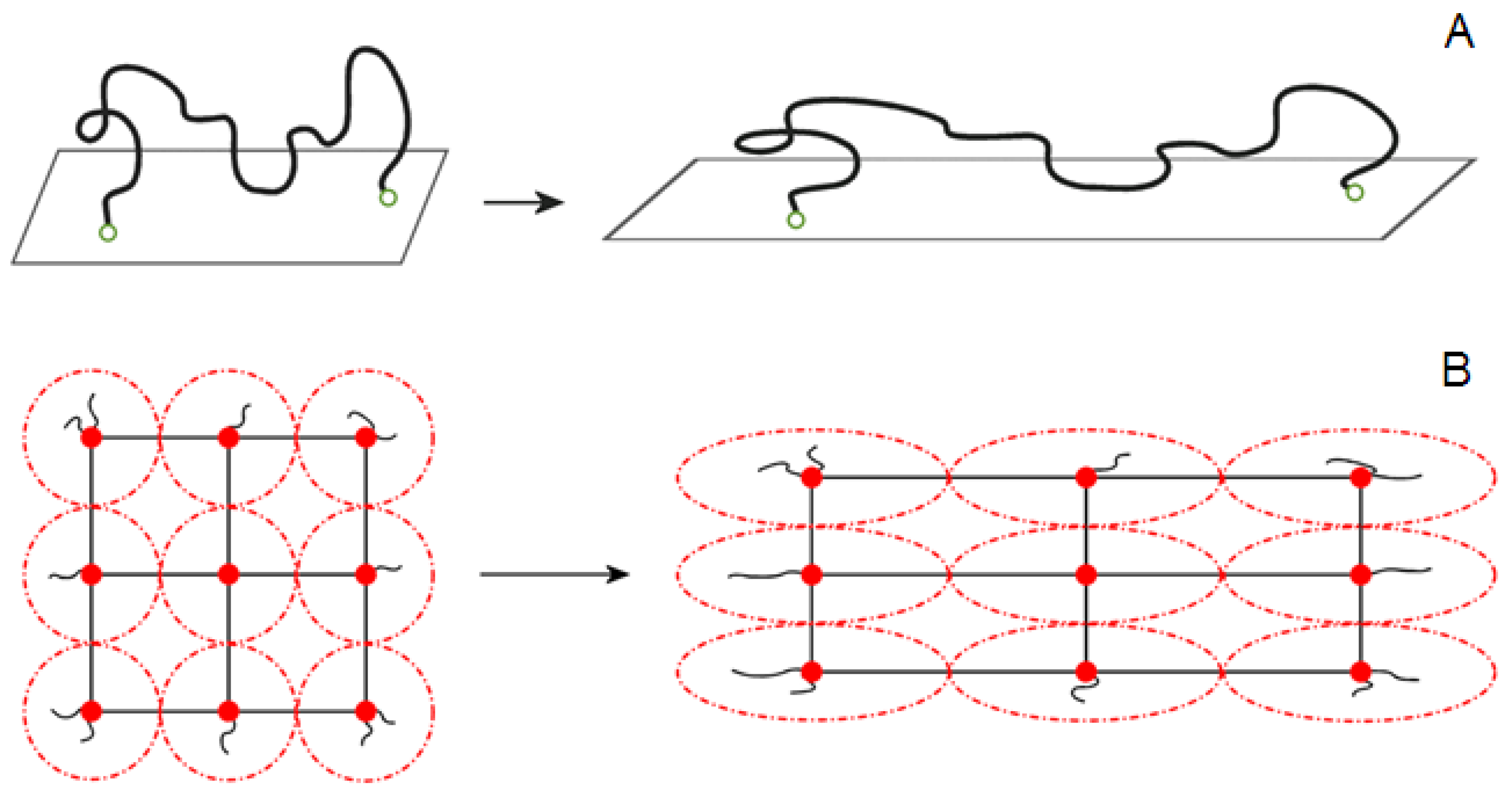
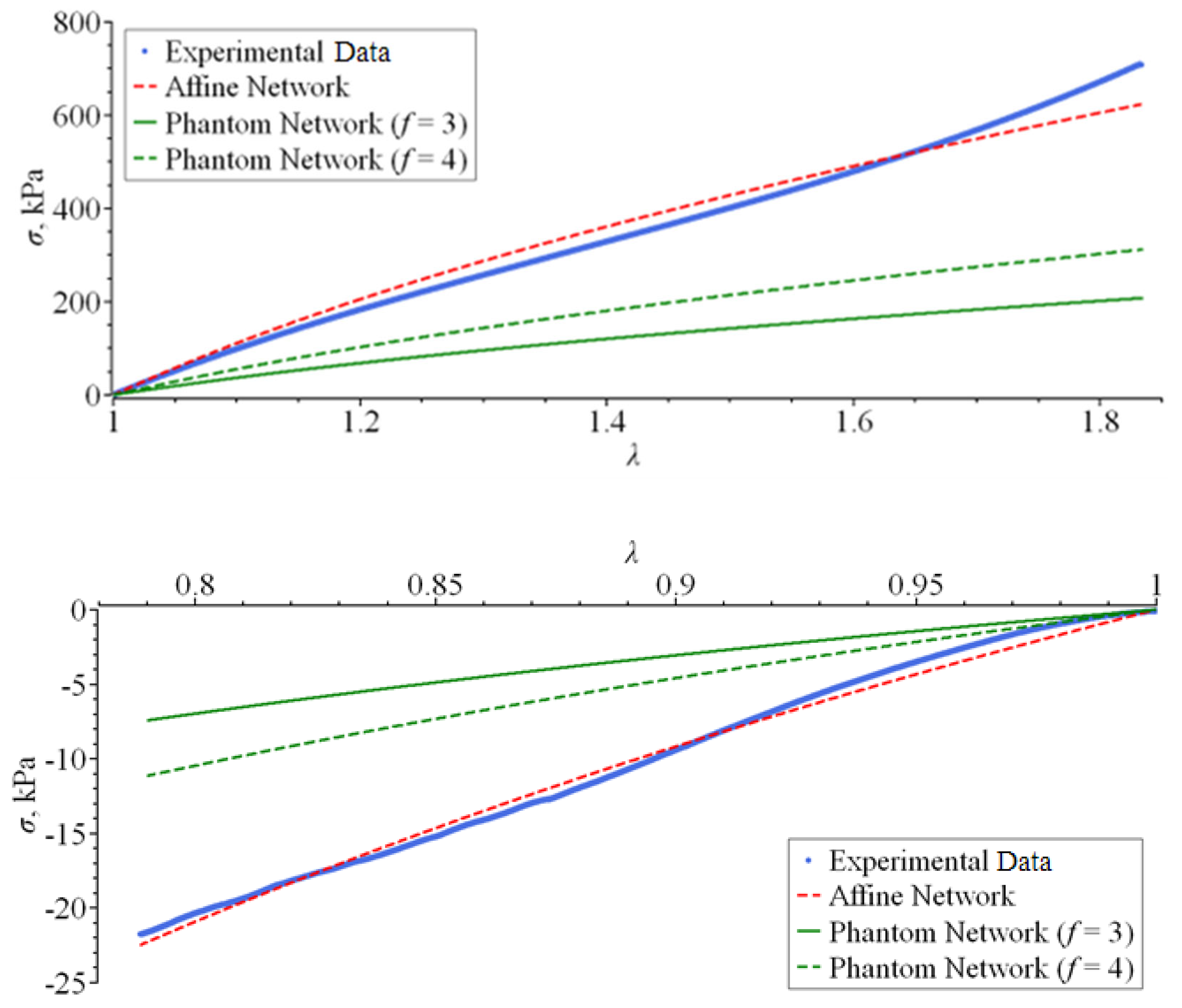
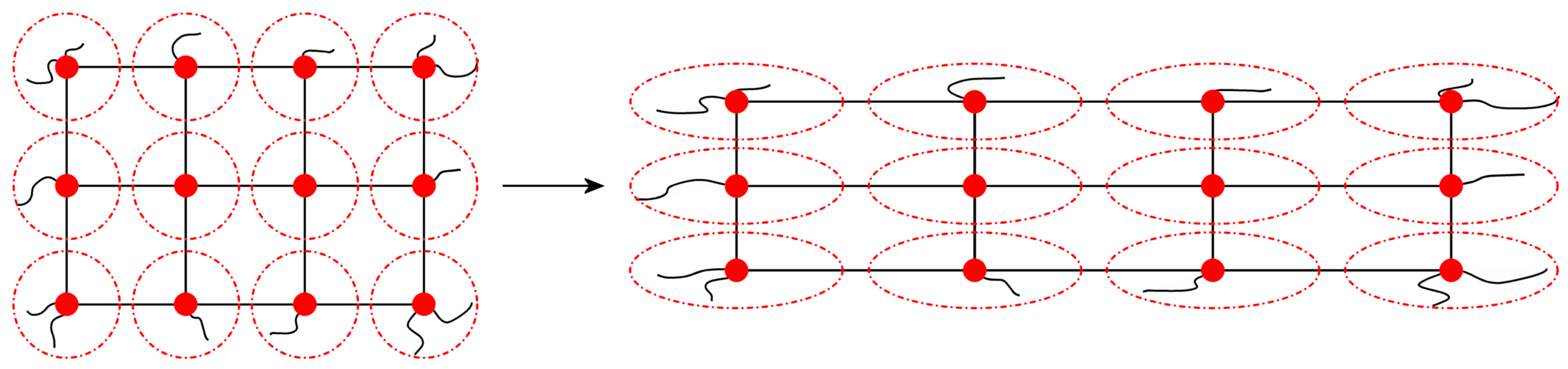
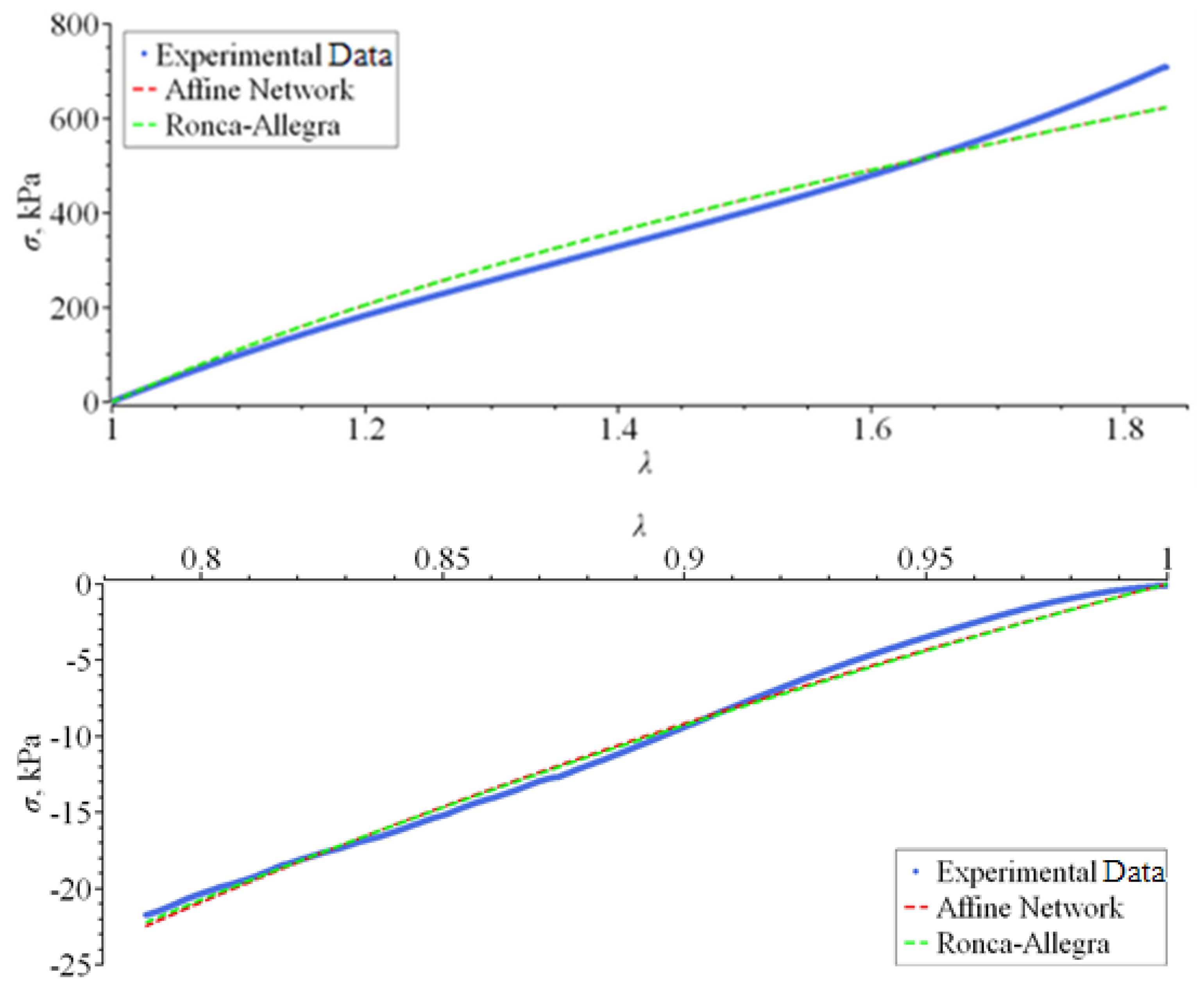
3.1. The Affine Network Model
3.2. Derivation of the Stress–Strain Equation for the Flory Affine Model
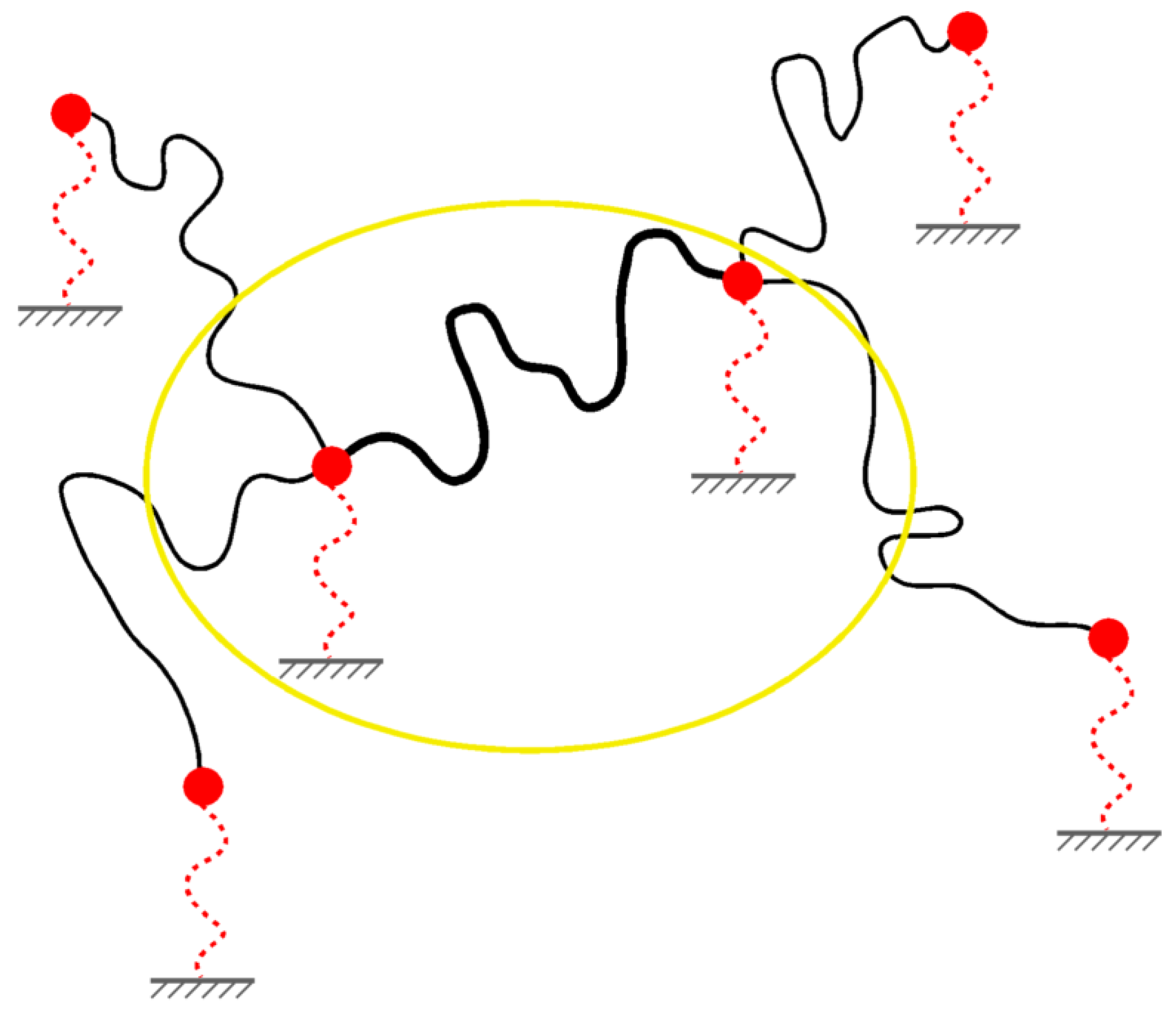
3.3. The Phantom Network Model
3.4. The Constrained Junction Models
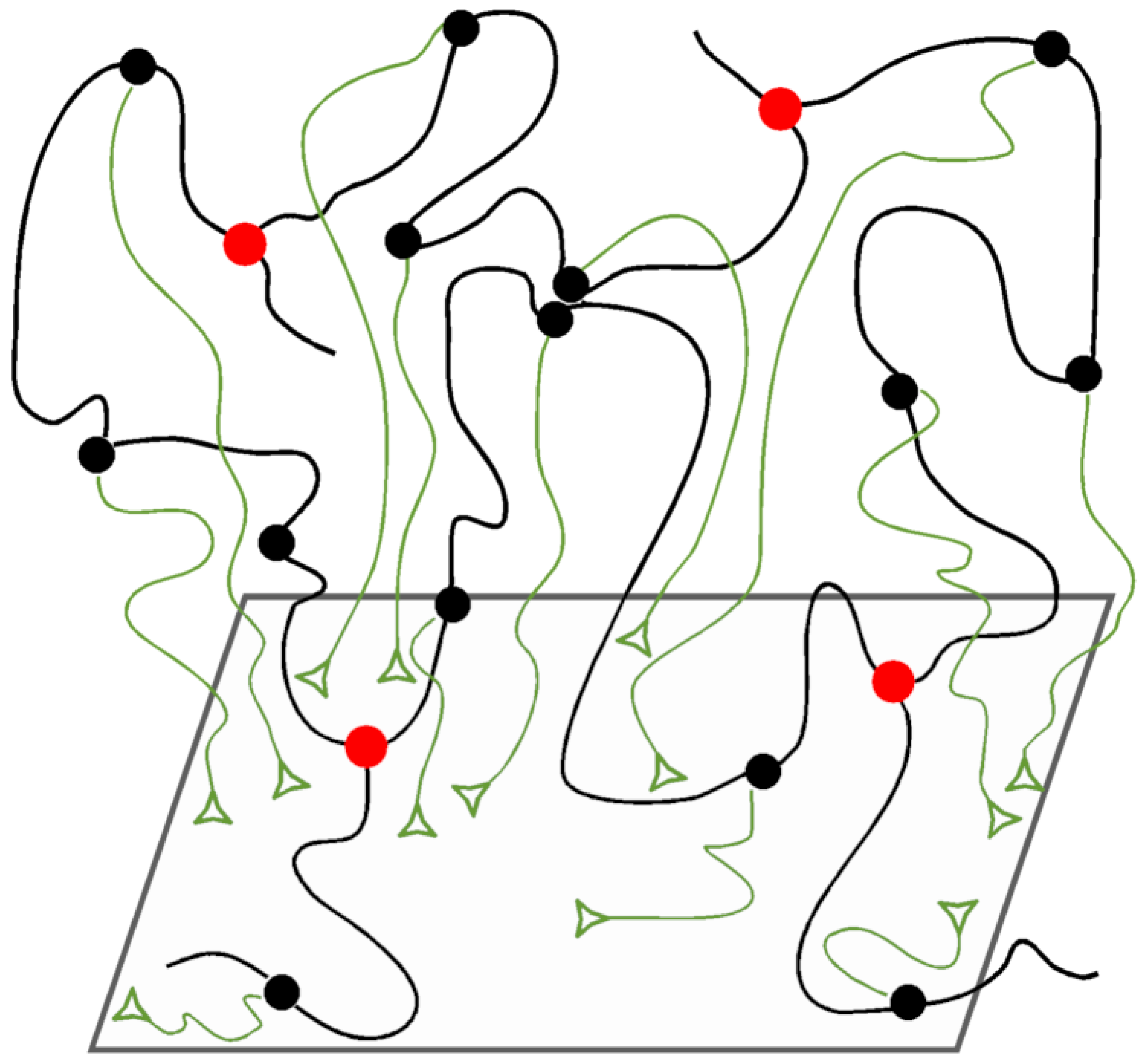
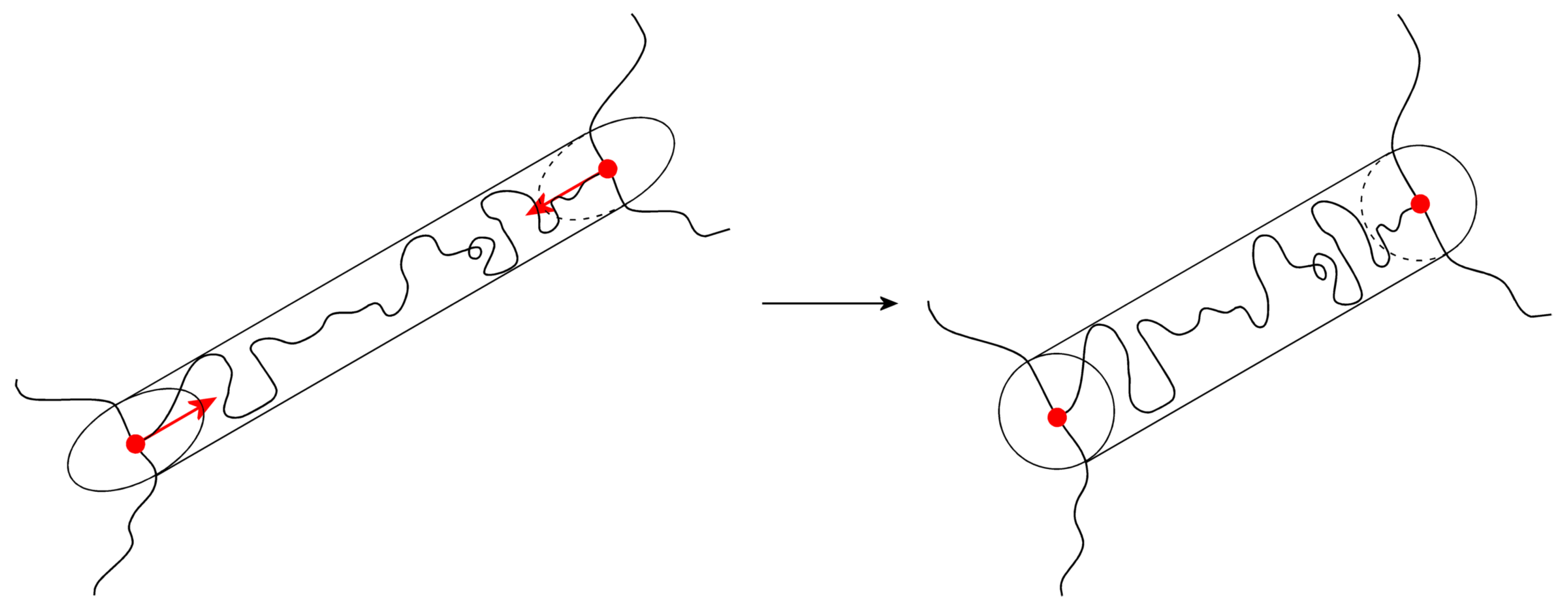
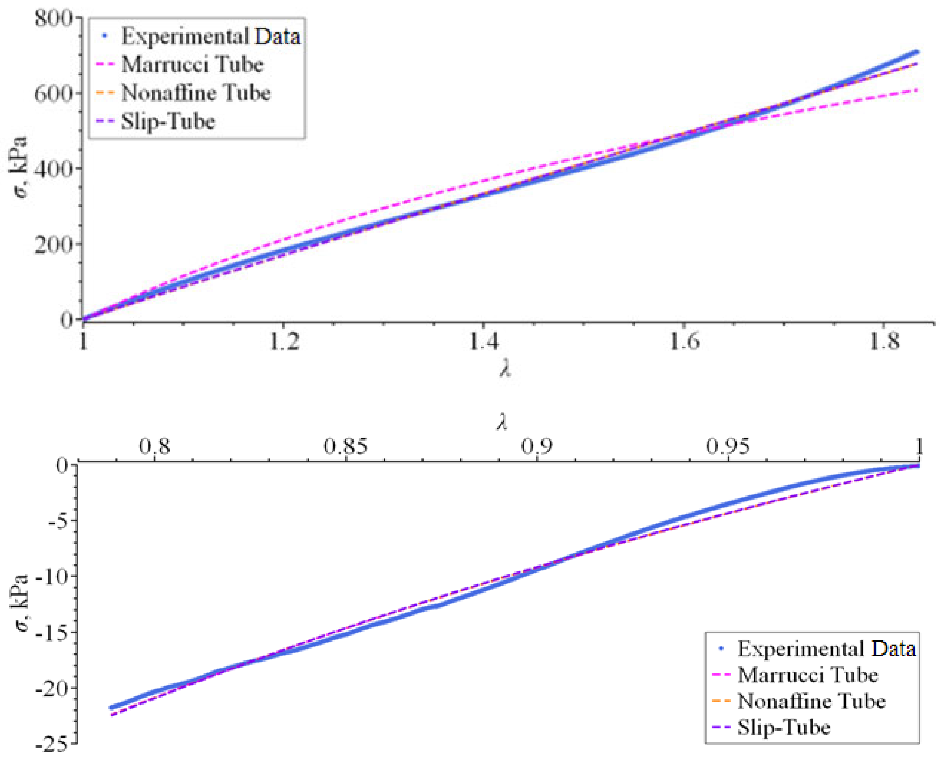
3.5. The Tube Models
3.6. The Slip-Link Models
3.7. The Nonaffine Tube Model
3.8. The Nonaffine Slip–Tube Model
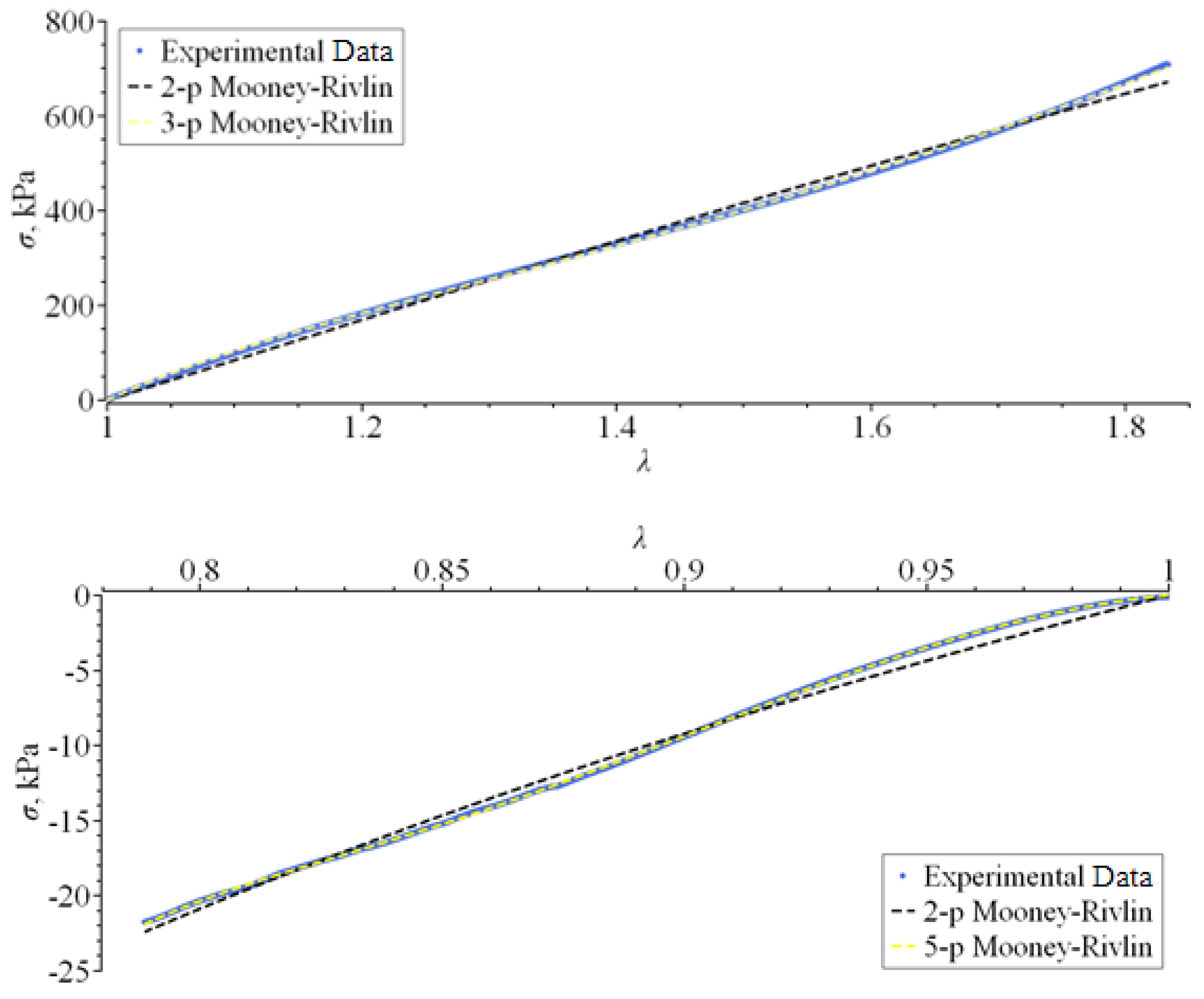
3.9. The Mooney–Rivlin Models
4. Conclusions
Funding
Acknowledgments
Conflicts of Interest
References
- Staudinger, H. Über Polymerisation. Ber. Dtsch. Chem. Ges. 1920, 53, 1073–1085. [Google Scholar] [CrossRef]
- Kuhn, W. Über die Gestalt fadenförmiger Moleküle in Lösungen. Kolloid Zeitschrift 1934, 68, 2–15. [Google Scholar] [CrossRef]
- Kuhn, W. Dependence of the Average Transversal on the Longitudinal Dimensions of Statistical Coils Formed by Chain Molecules. J. Polym. Sci. 1946, 1, 380–388. [Google Scholar] [CrossRef]
- de Gennes, P.-G. Scaling Concepts in Polymer Physics; Cornell University Press: Ithaca, NY, USA, 1979. [Google Scholar]
- Grizzuti, N. Reologia dei Materiali Polimerici: Scienza ed Ingegneria; Edizioni Nuova Cultura: Roma, Italy, 2012. [Google Scholar]
- Villani, V. Introduzione alla Scienza dei Materiali Polimerici; Aracne Editrice: Roma, Italy, 2017. [Google Scholar]
- Treloar, L.R.G. The Physics of Rubber Elasticity, 3rd ed.; Oxford University Press: Oxford, UK, 1975. [Google Scholar]
- Mark, J.E. Physical Properties of Polymers Handbook, 2nd ed.; Springer: New York, NY, USA, 2007. [Google Scholar]
- Mark, J.E.; Erman, B.; Roland, C.M. The Science and Technology of Rubber, 4th ed.; Elsevier Academic Press: Waltham, MA, USA, 2013. [Google Scholar]
- Erman, B.; Mark, J.E. Structure and Properties of Rubberlike Networks; Oxford University Press: New York, NY, USA, 1997. [Google Scholar]
- Ali, A.; Hosseini, M.; Sahari, B.B. A review and comparison on some rubber elasticity models. J. Sci. Ind. Res. 2010, 69, 495–500. [Google Scholar]
- Gedde, U.W.; Hedenqvist, M.S. Fundamental Polymer Science, 2nd ed.; Springer: Cham, Switzerland, 2019. [Google Scholar]
- Zhong, M.; Wang, R.; Kawamoto, K.; Olsen, B.D.; Johnson, J.A. Quantifying the impact of molecular defects on polymer network elasticity. Science 2016, 353, 1264–1268. [Google Scholar] [CrossRef]
- Lin, T.-S.; Wang, R.; Johnson, J.A.; Olsen, B.D. Revisiting the Elasticity Theory for Real Gaussian Phantom Networks. Macromolecules 2019, 52, 1685–1694. [Google Scholar] [CrossRef]
- Marrucci, G. Rubber Elasticity Theory. A Network of Entangled Chains. Macromolecules 1981, 14, 434–442. [Google Scholar] [CrossRef]
- Rubinstein, M.; Panyukov, S.V. Nonaffine Deformation and Elasticity of Polymer Networks. Macromolecules 1997, 30, 8036–8044. [Google Scholar] [CrossRef]
- Rubinstein, M.; Panyukov, S. Elasticity of Polymer Networks. Macromolecules 2002, 35, 6670–6686. [Google Scholar] [CrossRef]
- Mooney, M. The Thermodynamics of a Strained Elastomer. I. General Analysis. J. Appl. Phys. 1948, 19, 434–444. [Google Scholar] [CrossRef]
- Rivlin, R.S.; Rideal, E.K. Large elastic deformations of isotropic materials IV. Further developments of the general theory. Philos. Trans. R. Soc. A 1948, 241, 379–397. [Google Scholar]
- Villani, V.; Lavallata, V. Unusual Rheological Properties of Lightly Crosslinked Polydimethylsiloxane. Macromol. Chem. Phys. 2017, 218, 1700037. [Google Scholar] [CrossRef]
- Villani, V.; Lavallata, V. Unexpected Rheology of Polydimethylsiloxane Liquid Blends. Macromol. Chem. Phys. 2018, 219, 1700623. [Google Scholar] [CrossRef]
- Villani, V.; Lavallata, V. Entanglement Locking in the Unique Elasticity of Polydimethylsiloxane Rubbers. Macromol. Chem. Phys. 2020, 221, 1900497. [Google Scholar] [CrossRef]
- Elias, H.-G.; Mülhaupt, R. Ullmann’s Polymers and Plastics; Wiley-VCH: Weinheim, Germany, 2016. [Google Scholar]
- Wall, F.T.; Flory, P.J. Statistical Thermodynamics of Rubber Elasticity. J. Chem. Phys. 1951, 19, 1435–1439. [Google Scholar] [CrossRef]
- Flory, P.J. Statistical thermodynamics of random networks. Proc. R. Soc. Lond. A 1976, 351, 351–380. [Google Scholar]
- James, H.M.; Guth, E. Theory of the Elastic Properties of Rubber. J. Chem. Phys. 1943, 11, 455–481. [Google Scholar] [CrossRef]
- James, H.M. Statistical Properties of Networks of Flexible Chains. J. Chem. Phys. 1947, 15, 651–668. [Google Scholar] [CrossRef]
- James, H.M.; Guth, E. Theory of the Increase in Rigidity of Rubber during Cure. J. Chem. Phys. 1947, 15, 669–683. [Google Scholar] [CrossRef]
- Halary, J.L.; Laupretre, F.; Monnerie, L. Polymer Materials Macroscopic Properties and Molecular Interpretations; Wiley: New York, NY, USA, 2011. [Google Scholar]
- Lang, M. Relation between Cross-Link Fluctuations and Elasticity in Entangled Polymer Networks. Macromolecules 2017, 50, 2547–2555. [Google Scholar] [CrossRef]
- Mark, J.; Ngai, K.; Graessley, W.; Mandelkern, L.; Samulski, E.; Koenig, J.; Wignall, G. Physical Properties of Polymers, 3rd ed.; Cambridge University Press: Cambridge, UK, 2004. [Google Scholar]
- Saccomandi, G.; Ogden, R.W. Mechanics and Thermomechanics of Rubberlike Solids; Springer: Wien, Austria, 2004. [Google Scholar]
- Mark, J.E.; Erman, B. Rubberlike Elasticity a Molecular Primer, 2nd ed.; Cambridge University Press: Cambridge, UK, 2007. [Google Scholar]
- Properties and Behavior of Polymers; Wiley: Hoboken, NJ, USA, 2011.
- Ronca, G.; Allegra, G. An approach to rubber elasticity with internal constraints. J. Chem. Phys. 1975, 63, 4990–4997. [Google Scholar] [CrossRef]
- Erman, B.; Flory, P.J. Theory of elasticity of polymer networks. II. The effect of geometric constraints on junctions. J. Chem. Phys. 1978, 68, 5363–5369. [Google Scholar] [CrossRef]
- Flory, P.J. Molecular Theory of Rubber Elasticity. Polym. J. 1985, 17, 1317–1320. [Google Scholar] [CrossRef]
- Flory, P.J. Network topology and the theory of rubber elasticity. Br. Polym. J. 1985, 17, 96–102. [Google Scholar] [CrossRef]
- Erman, B.; Mark, J.E. Rubber-like Elasticity. Ann. Rev. Phys. Chem. 1989, 40, 351–374. [Google Scholar] [CrossRef]
- Flory, P.J. Theory of elasticity of polymer networks. The effect of local constraints on junctions. J. Chem. Phys. 1977, 66, 5720–5729. [Google Scholar] [CrossRef]
- Roland, C.M. Viscoelastic Behavior of Rubbery Materials; Oxford University Press: Oxford, UK, 2011. [Google Scholar]
- Erman, B.; Monnerie, L. Theory of elasticity of amorphous networks: Effect of constraints along chains. Macromolecules 1989, 22, 3342–3348. [Google Scholar] [CrossRef]
- Fontaine, F.; Noel, C.; Monnerie, L.; Erman, B. Stress-strain-swelling behaviour of amorphous polymeric networks: Comparison of experimental data with theory. Macromolecules 1989, 22, 3352–3355. [Google Scholar] [CrossRef]
- Erman, B.; Monnerie, L. Theory of Elasticity of amorphous networks: Effects of Constraints along Chains. Macromolecules 1992, 25, 4456. [Google Scholar] [CrossRef]
- Kloczkowski, A.; Mark, J.E.; Erman, B. A Diffused-Constraint Theory for the Elasticity of Amorphous Polymer Networks. 1. Fundamentals and Stress-Strain Isotherms in Elongation. Macromolecules 1995, 28, 5089–5096. [Google Scholar] [CrossRef]
- Edwards, S.F. The statistical mechanics of polymerized material. Proc. Phys. Soc. 1967, 92, 9–16. [Google Scholar] [CrossRef]
- Edwards, S.F.; Vilgis, T.A. The tube model theory of rubber elasticity. Rep. Prog. Phys. 1988, 51, 243–297. [Google Scholar] [CrossRef]
- Graessley, W.W. Polymeric Liquids & Networks: Structure and Properties; Garland Science: New York, NY, USA, 2004. [Google Scholar]
- Edwards, S.F.; Vilgis, T.A. The effect of entanglements in rubber elasticity. Polymer 1986, 27, 483–492. [Google Scholar] [CrossRef]
- Dossin, L.M.; Graessley, W.W. Rubber Elasticity of Well-Characterized Polybutadiene Networks. Macromolecules 1979, 12, 123–130. [Google Scholar] [CrossRef]
- Queslel, J.P.; Mark, J.E. Encyclopedia of Polymer Science and Technology; Mark, H.F., Ed.; Wiley: Hoboken, NJ, USA, 2014. [Google Scholar]
- Doi, M. Explanation for the 3.4-power law for viscosity of polymeric liquids on the basis of the tube mode. J. Polym. Sci. Polym. Phys. Ed. 1983, 21, 667–684. [Google Scholar] [CrossRef]
- Rubinstein, M.; Colby, R.H. Polymer Physics; Oxford University Press: Oxford, UK, 2003. [Google Scholar]
- Bueche, F. Physical Properties of Polymers; Interscience Publishers: New York, NY, USA, 1962. [Google Scholar]
- Sperling, L.H. Introduction to Physical Polymer Science, 4th ed.; Wiley: Hoboken, NJ, USA, 2006. [Google Scholar]
- Gnanou, Y.; Fontanille, M. Organic and Physical Chemistry of Polymers; Wiley: Hoboken, NJ, USA, 2008. [Google Scholar]
- Mooney, M. A Theory of Large Elastic Deformation. J. Appl. Phys. 1940, 11, 582–592. [Google Scholar] [CrossRef]
- Wagner, M.H. The origin of the C2 term in rubber elasticity. J. Rheol. 1994, 38, 655–679. [Google Scholar] [CrossRef]
- Donald, B.J.M. Practical Stress Analysis with Finite Elements; Glasnevin Publishing: Dublin, Ireland, 2007. [Google Scholar]
- Kumar, N.; Rao, V.V. Hyperelastic Mooney-Rivlin Model: Determination and Physical Interpretation of Material Constants. MIT Int. J. Mech. Eng. 2016, 6, 43–46. [Google Scholar]
- Szurgott, P.; Jarzębski, Ł. Selection of a Hyper-Elastic Material Model—A Case Study for Polyurethane Component. Lat. Am. J. Solids Struct. 2019, 16, e191. [Google Scholar] [CrossRef]
- Svaneborg, C.; Everaers, R.; Grest, G.S.; Curro, J.G. Connectivity and Entanglement Stress Contributions in Strained Polymer Networks. Macromolecules 2008, 41, 4920–4928. [Google Scholar] [CrossRef]
- Yoo, S.H.; Yee, L.; Cohen, C. Effect of network structure on the stress-strain behaviour of endlinked PDMS elastomers. Polymer 2010, 51, 1608–1613. [Google Scholar] [CrossRef]
- Sliozberg, Y.R.; Mrozek, R.A.; Schieber, J.D.; Kröger, M.; Lenhart, J.L.; Andzelm, J.W. Effect of polymer solvent on the mechanical properties of entangled polymer gels: Coarse-grained molecular simulation. Polymer 2013, 54, 2555–2564. [Google Scholar] [CrossRef]
- Wittmer, J.P.; Beckrich, P.; Meyer, H.; Cavallo, A.; Johner, A.; Baschnagel, J. Intramolecular long-range correlations in polymer melts: The segmental size distribution and its moments. Phys. Rev. E 2007, 76, 011803. [Google Scholar] [CrossRef] [PubMed]
- Mezzasalma, S.A.; Abramic, M.; Grassi, G.; Grassi, M. Rubber Elasticity of Polymer Networks in Explicitly non-Gaussian States. Statistical Mechanics and LF-NMR Inquiry in Hydrogel Systems. Int. J. Eng. Sci. 2022, 176, 103676. [Google Scholar] [CrossRef]
- Bock, W.; da Silva, J.L.; Streit, L. On the potential in non-Gaussian chain polymer models. Math. Methods Appl. Sci. 2019, 42, 7452–7460. [Google Scholar] [CrossRef]


| Model | Constitutive Stress–Strain Equation | R2 |
|---|---|---|
| Affine Network | 0.97608 | |
| Ronca–Allegra | 0.97608 | |
| Marrucci Tube (r = 1) | 0.96526 | |
| Nonaffine Tube | 0.99649 | |
| Nonaffine Slip–Tube | 0.99663 | |
| Two-parameter Mooney–Rivlin | 0.99531 | |
| Three-parameter Mooney–Rivlin | 0.99978 |
| Model | Stress–Strain Constitutive Equation | R2 |
|---|---|---|
| Affine Network | 0.99299 | |
| Ronca–Allegra | 0.99317 | |
| Marrucci Tube (r = 1) | 0.99308 | |
| Nonaffine Tube | 0.99299 | |
| Nonaffine Slip–Tube | 0.99299 | |
| Two-parameter Mooney–Rivlin | 0.99301 | |
| Five-parameter Mooney–Rivlin | 0.99994 |
Disclaimer/Publisher’s Note: The statements, opinions and data contained in all publications are solely those of the individual author(s) and contributor(s) and not of MDPI and/or the editor(s). MDPI and/or the editor(s) disclaim responsibility for any injury to people or property resulting from any ideas, methods, instructions or products referred to in the content. |
© 2024 by the authors. Licensee MDPI, Basel, Switzerland. This article is an open access article distributed under the terms and conditions of the Creative Commons Attribution (CC BY) license (https://creativecommons.org/licenses/by/4.0/).
Share and Cite
Villani, V.; Lavallata, V. The Theories of Rubber Elasticity and the Goodness of Their Constitutive Stress–Strain Equations. Physchem 2024, 4, 296-318. https://doi.org/10.3390/physchem4030021
Villani V, Lavallata V. The Theories of Rubber Elasticity and the Goodness of Their Constitutive Stress–Strain Equations. Physchem. 2024; 4(3):296-318. https://doi.org/10.3390/physchem4030021
Chicago/Turabian StyleVillani, Vincenzo, and Vito Lavallata. 2024. "The Theories of Rubber Elasticity and the Goodness of Their Constitutive Stress–Strain Equations" Physchem 4, no. 3: 296-318. https://doi.org/10.3390/physchem4030021