Evaluating OSM Building Footprint Data Quality in Québec Province, Canada from 2018 to 2023: A Comparative Study

Abstract

OpenStreetMap (OSM) is among the most prominent Volunteered Geographic Information (VGI) initiatives, aiming to create a freely accessible world map. Despite its success, the data quality of OSM remains variable. This study begins by identifying the quality metrics proposed by earlier research to assess the quality of OSM building footprints. It then evaluates the quality of OSM building data from 2018 and 2023 for five cities within Québec, Canada. The analysis reveals a significant quality improvement over time. In 2018, the completeness of OSM building footprints in the examined cities averaged around 5%, while by 2023, it had increased to approximately 35%. However, this improvement was not evenly distributed. For example, Shawinigan saw its completeness surge from 2% to 99%. The study also finds that OSM contributors were more likely to digitize larger buildings before smaller ones. Positional accuracy saw enhancement, with the average error shrinking from 3.7 m in 2018 to 2.3 m in 2023. The average distance measure suggests a modest increase in shape accuracy over the same period. Overall, while the quality of OSM building footprints has indeed improved, this study shows that the extent of the improvement varied significantly across different cities. Shawinigan experienced a substantial increase in data quality compared to its counterparts.

1. Introduction

The term “Volunteered Geographic Information” (VGI) was coined by Goodchild to describe the process of geographic data production by members of the general public [1]. This new term also acknowledges that VGI data are collected voluntarily by masses of individuals. The scope of VGI is extensive, encompassing data types such as personal trajectories, geotagged photographs, and elements of online maps that have been digitized by volunteers [2]. VGI can be categorized into three groups based on data content: text-based VGI, image-based VGI, and map-based VGI [3,4]. Text-based VGI might take the form of a georeferenced tweet, whereas image-based VGI could be exemplified by a geotagged photo. Map-based VGI typically involves online communities where contributors are able to edit, create, and delete map features. Indeed, map-based VGI represents a geographically explicit form of VGI, where the contributors actively engage in generating geographic content [5].

A prime example of web-based VGI is OpenStreetMap, which was created by Steve Coast and is a free, editable map of the world that is open to all [6]. OSM enables contributors to edit, create, and delete content on the world map. Numerous studies have demonstrated that contributions to OSM are not uniform, revealing areas with substantial activity as well as those with minimal contributions [7,8].

There are no prerequisites for becoming a contributor to the OSM project. As a result, many contributors may lack geographic knowledge and are not necessarily versed in the rules and procedures of spatial data collection [9]. Consequently, the quality of spatial data in the OSM project cannot be assured. Additionally, a small number of vandalism cases, where errors are introduced into the OSM map intentionally, have been detected [8].

Conversely, it is impractical to utilize spatial data in any application without ensuring that the data quality meets the application’s requirements. The efficient use of OSM data hinges on the understanding of its quality. Therefore, assessing the quality of OSM data is imperative.

A range of studies has been conducted to evaluate the quality of OSM data across various regions of the world [10,11,12,13,14,15,16]. One of the first evaluations of the quality of OSM buildings was conducted by Fan et al. [12]. They not only evaluated the completeness, semantic accuracy, and positional accuracy of OSM buildings, but also introduced the turning function approach to assess shape similarity, thereby enhancing the evaluation of shape accuracy. Brovelli and Zamboni [17] proposed a novel method based on coordinate transformation to identify the corresponding edges and vertices between features in OSM and the reference database. Jacobs [18] evaluated the quality of OSM building footprint data in Ottawa city. Tian et al. [19] assessed the completeness and spatial patterns of OSM building data in China, discovering a twentyfold increase in building count from 2012 to 2017. Their findings also revealed a correlation between economic factors, OSM road length, and the proliferation of OSM building data [19].

Borkowska, Bielecka and Pokonieczny [20] conducted an assessment of the completeness of OSM buildings in Poland, noting that many developed urban areas boasted a 100% completion rate. Conversely, lower completeness rates were prevalent in less urbanized regions. This pattern suggests that OSM building completeness tends to be greater in more developed areas. Biljecki et al. [21] found that the completeness of building attributes in OSM varies significantly, being very high in some areas but notably low in others, indicating a high degree of heterogeneity in OSM attribute completeness [21]. The study revealed that OSM contributors predominantly recorded the number of floors and the building type for OSM structures [21]. A number of researchers have further concentrated on the attribute data of OSM buildings, attempting to predict the building types, such as residential or commercial ones, in cases where the attribute values for building type are missing [22,23,24].

Another research evaluated the quality of OSM building data in Taiwan [25]. Researchers have attempted to discern the relationship between the quality of OSM building data and indicators like the density of building footprints (Zhou, 2018) [15]. Herfort et al. [26] investigated the completeness of OSM building data across the globe and found that, among almost 13,000 urban agglomerations, 1848 urban centers had a completeness exceeding 80%, while 9163 cities had less than 20% completeness [26]. It shows that the completeness of OSM building footprint data is heterogenous. Küçük and Anbaroğlu [27] evaluated the spatial accuracy of OSM buildings in Ankara, Turkey, and determined that the average error is 9.5 m.

Maidaneh Abdi et al. [28] posited a relationship between the extrinsic and intrinsic quality measures of OSM data. By attempting to predict the extrinsic quality measures using intrinsic ones, which do not require reference data, their methodology yielded predictions of extrinsic quality with 30% less variance compared to a baseline uninformed predictor [28].

In regions where authoritative data are lacking, the feasibility of conducting quality assessments of OpenStreetMap (OSM) through direct comparison with such data is limited. This challenge has prompted researchers to investigate alternative methods, seeking quality indicators that can offer insights into the OSM quality in these data-scarce areas [15,29,30,31,32,33].

Given that contributors are constantly updating the map, OSM features undergo continuous edits, leading to ongoing changes in the quality of OSM data over time. Hecht et al. [34] evaluated how the quality of OSM database changes over time. They found that the completeness of OSM building footprints in Saxony, Germany, increased from 15% in 2011 to 23% in 2012 [34]. Herfort, B. et al. [26] conducted extensive research to determine how the completeness of OSM urban building data has changed over time. They evaluated 13,189 urban centers worldwide. Their findings indicate that while there was an overall increase in completeness for many urban centers, significant disparities were observed across different regions. Additionally, they noted that before 2014, the spatial inequality of OSM buildings increased, but after 2014, it became more even [26]. Tian et al. [19] compared the OSM building data in China between 2012 and 2017 and found that the volume of data had increased twentyfold. It was observed that the majority of these changes occurred along the east coast of China.

While numerous studies have analyzed the improvement of OpenStreetMap quality over time, there appears to be a gap in comprehensive research focusing on the improvement of various aspects of OSM building data quality, such as the shape and positional accuracy, particularly in Québec.

Consequently, this research undertakes a comparative analysis of four quality measures: completeness, positional accuracy, shape accuracy, and attribute accuracy, over a five-year period. This approach aims to shed light on how the quality of OSM building data has evolved during this time, using these quality measures. Therefore, the central question of this research is: How has the quality of OSM building data in Québec changed between 2018 and 2023, when evaluated from these four different quality perspectives?

The structure of the remainder of this research is organized into three main sections. Section 2: This section undertakes a literature review to identify the measures that previous researchers have proposed for assessing the quality of OSM building data. Section 3: The OSM datasets for the years 2018 and 2023 are acquired for five cities in Québec, Canada, including Québec City, Longueuil, Repentigny, Rouyn-Noranda, and Shawinigan. These datasets are subsequently compared with authoritative data to evaluate the quality measures in the Québec Province for both years. Section 4: An analysis of the results is conducted to ascertain the extent to which the quality of OSM data has improved between 2018 and 2023.

2. Materials and Methods

2.1. Correspondence Types

The relationship between OSM features and reference features can be complicated because the majority of OSM data are digitized from aerial images and the contributors draw the footprint of buildings based on a photo of their roof. Thus, sometimes a group of adjacent buildings is represented as one building in OSM or vice versa. Fan et al. [12] argued that the relationship between OSM footprints and the footprints in the reference databases can be one of the following cases: (OSM: reference)

• 1:1—this relationship exists when one OSM building is matched to only one reference, and that reference building also matches to only one OSM building;
• 1:0—this case is when there is a building on OSM that has no corresponding polygon in the reference database (data commission);
• 1:n—this case happens when one OSM feature is corresponding to more than one feature in the reference database;
• 0:1—this case is the opposite of the (1:0) relationship (data omission);
• n:1—this case is the opposite of the (1:n) relationship;
• n:m—this case means that a number of buildings in OSM are matching to a number of buildings in the reference database.

In the case of OpenStreetMap, the purpose of feature matching is to find out which of the abovementioned correspondence types applies to the building footprint of OSM and the corresponding one(s) in the reference database.

2.2. Feature Matching

Feature matching is a process that aims to find corresponding features between multiple databases [12]. The majority of studies on OSM building data [15,18,25,35] used the feature matching method that is introduced by [12], which is based on the area of the overlapping part of the two polygons. This method is based on the fact that the polygon displacement between OSM and the reference database is not considerable [12]. Therefore, the area where the two polygons overlap can be used as a criterion for finding the corresponding features [12]. Fan et al. [12] considered a tolerance of 30%, which means if two polygons have more than 30% overlap, they are considered corresponding polygons. The following equation is proposed by Fan et al. [12] for finding corresponding building footprints:

$$\frac{{Area}_{overlap}}{Min(Area\left({Foot}_{osm\_i}\right),Area({foot}_{ref\text{\_}j}\left)\right)}>30\%$$

(1)

The overlap method has a great accuracy when the corresponding types are simple (1:1, 1:0, 0:1); however, when the correspondence type is more complicated (1:n, n:m, n:1) or when there is a considerable displacement between the OSM and the reference polygon, the accuracy of the overlap method reduces [36]. Moradi et al. [36] proposed a feature matching algorithm for OSM buildings that uses not only the overlap between two polygons, but also measures the degree to which the two shapes are similar. In this research, the method proposed by Moradi et al. [36] is used to perform a more accurate feature matching between OSM and the reference building footprints.

2.3. Completeness

Completeness refers to whether or not the objects in the real world and their attributes exist in the database [37]. Completeness has two main components: data completeness and model completeness [37]. In this study, only data completeness for building footprints is evaluated. Attribute completeness expresses how completely the attributes that describe the characteristics of a feature exist in the database [37]. Two main issues are related to completeness evaluation of the data: commission and omission [38]. Commission is when the object in the database does not exist in the real world and omission happens when an object in the real world is not mapped in the database [38]. In the case of building footprints of the OSM database, completeness means how complete the buildings of the study area are mapped by the OSM contributors.

There are two common methods for evaluating the completeness of OSM building footprints: the area-based method and object-based method [34]. The area-based method compares the total area of the building polygons of the OSM database to the total area of the building footprints of the reference database in the study area [34]. The object-based method compares the total number of the OSM buildings in an area to the total number of buildings in the reference database in that area [34]. The area-based method is easier because it does not require feature matching and it just compares the total area of the polygons of the two databases. However, the object-based method requires finding the corresponding features before comparing numbers. Hechtet et al. [34] compared the two methods and suggested the use of an object-based method because the area-based method is highly sensitive to disparities between the building footprints in OSM and building footprints in the reference databases. Törnros et al. [13] compared the two methods of completeness evaluation and found that neither of them pays attention to the geometrical representation of the buildings. Therefore, both methods have shortcomings that may result in the overestimation or underestimation of the completeness [13]. For example, when a block of buildings in the real world are represented with just one polygon in OSM, comparing the total number of buildings may underestimate the completeness [13]. Törnros et al. [13] proposed to merge the adjoining buildings in both databases and then compare the resulting polygons and calculate three parameters : true positive, false negative and false positive. This method tries to solve the problem where sometimes adjoining buildings are represented by only one polygon.

2.3.1. Area-Based Method

In the area-based method, the completeness is simply calculated based on the ratio of the total area of buildings in OSM to the total area of buildings in the reference database [18]. This method is not computationally heavy. However, a number of issues can cause uncertainty in the results [13]. Area-based completeness can be calculated using the following equation [34]:

$$C_{Area}=\frac{{\sum }_{i=1}^{n}Area\left({footprint}_{OSM}\right)}{{\sum }_{j=1}^{m}Area\left({footprint}_{Reference}\right)}$$

(2)

where n is the number of buildings in OSM and m is the number of buildings in the reference database. A number of research studies applied the area-based method for assessing the completeness of OSM building footprints [12,18,34,39].

2.3.2. Object-Based Method

In the object-based method, first, the corresponding features are detected. Then, the completeness is calculated based on the comparison between the number of the features in OSM and their number in the reference database. Therefore, it is more reliable for completeness assessment [34]. The object-based completeness evaluation of OSM buildings can be carried out using the following equation [34]:

$$Completeness=\frac{NumberoffeaturesinOSM}{NumberoffeaturesinreferenceDB}$$

(3)

This method can calculate omission and commission much more accurately than the area-based method because in this method, the features are matched and the corresponding types are known.

2.4. Positional Accuracy

In GIS, the position of an object in the real world is measured with respect to an appropriate coordinate system and is stored in the databases [37]. The position of the objects of the real world can be obtained via repeated measurements [37]. The precision of the position refers to the spread of the results obtained by the measurements [37]. However, accuracy is the distance from the measured position to the true position (which is unknown) [37]. The ISO standard for spatial data quality defines positional accuracy as the accuracy of the position of objects with respect to a coordinate system [38]. Positional accuracy has three elements: absolute accuracy, relative accuracy, and gridded data positional accuracy [38]. Absolute accuracy is the closeness of the measured coordinates in comparison to the true coordinates, while the relative positional accuracy refers to the positional accuracy of the objects of the map with respect to the position of the other objects [38].

A number of research studies evaluated the positional accuracy of the OSM building footprints [2,12]. The common point among all these research studies is that they mostly used a reference database to compare with OSM. Fan et al. [12] evaluated the positional accuracy of building footprints of OSM by comparing the position of their corresponding vertices. Firstly, this method finds the corresponding vertices of the OSM polygon and the reference polygon. Then, it calculates the average distance of these points as a measure of the positional accuracy of the buildings [12]. Only the buildings with a 1:1 relation are included in the calculations. Finally, they calculated four measures, including the maximum offset, minimum offset, average offset, and standard deviation [12].

Brovelli and Zamboni [17] proposed a method for evaluating the positional accuracy of the OSM building footprints. In the first step, this method estimates the parameters of an affine transformation between OSM building vertices and the corresponding reference vertices [17]. A manual detection of more than four homologous points is required for each region of the map [17]. Finally, all the points of OSM are transformed using the affine transformation. Then, they are compared to the corresponding points of the reference database [17]. The distance between the two homologous points is the measure of positional accuracy in this method [17].

A simple but efficient method of positional accuracy assessment for building footprints of OSM is applied by Copes [2]. Copes [2] compared the position of the centroid of the building on OSM to the centroid of the corresponding building in the reference database. The distance between the two centroids can be used as an indicator for positional accuracy [2]. The measure of positional accuracy of this method is calculated as follows:

$$Distanc{e}_{average}=\frac{{\sum }_{i=1}^n\sqrt{{\left(X_{OSM}^i-X_{ref}^{corresponding}\right)}^2+{\left(Y_{osm}^i-Y_{osm}^{corresponding}\right)}^2}}{n}$$

(4)

where $X_{ref}^{corresponding}$ is the X coordinate of the centroid of the polygon in the reference database that is corresponding to the centroid of the ith polygon of OSM and n is the number of OSM buildings that have a 1:1 relationship with reference buildings.

The distance is not the only parameter that can be measured between the two centroids. Barronet et al. [40] proposed an intrinsic quality indicator that compares the displacement of the road junctions over the time. In a normal case, the displacement of the road junctions should be distributed uniformly in all directions [40]. However, vandalism can affect distribution in one direction more than others [40]. The authors believe that this method can be used for building centroids. Therefore, we propose to not only compare the distance between the two centroids, but also to evaluate the distribution of the directions. The evaluation of the directions can answer the question whether or not the buildings of OSM (compared to the reference ones) are displaced toward any specific direction.

2.5. Shape Accuracy

The buildings of OSM are usually digitized by the contributors from areal imageries. Fan et al. [12], and Törnros et al. [13], mentioned that the buildings of the OSM are in fact a simplified representation of the buildings of the reference database. Therefore, on one hand, the shapes of the polygons are not digitized with the same level of details as the reference database [12,39]. On the other hand, sometimes there are some errors in the digitization process due to the lack of geographic knowledge of the contributors or even vandalism activities. Thus, a shape dissimilarity can happen due to different reasons. It is necessary to evaluate how similar the shapes of the buildings in OSM are to the shapes of the buildings in the reference database.

Fan et al. [12] defined the shape accuracy as the similarity between the footprints in the two databases. Fan et al. [12] proposed the use of a turning function to measure the similarity of the polygons. This method was used by a number of other researchers [12,25,41]. This method represents each polygon with a set of tangents of the edges and the length of each edge [12]. The length of each edge should be normalized by the perimeter of the polygon so that different polygons can be compared [12]. The dissimilarity of two polygons can then be calculated by comparing these two functions.

Xu et al. [42] proposed using discrete Fourier transform for calculating the shape similarity between the two databases. This method first finds the polygons with 1:1 relationship. Then, each polygon will be considered as a signal and Fourier transformation is used to express that signal in terms of a complex exponential [42]. The measure of the similarity of the two polygons is then defined by the distance between the two exponentials [42]. This method is innovative but computationally heavy because there are many buildings in the province of Québec, and it takes a very long time to calculate Fourier transformation for all of them.

Siebritz [39] applied three measures to compare the building footprints of OSM and building footprints of the reference database. The first criterium is the ratio of the two areas [39]:

$$AreaRatio=\frac{{Area}_{osm}}{{Area}_{ref}}$$

(5)

This measure can indicate how the area of the two polygons is similar. However, this measure cannot indicate the difference in the shape of the two polygons. The second measure that is applied by [39] is compactness:

$$Compactness=\frac{Area}{(0.282\ast {Perimeter)}^2}$$

(6)

This measure can tell us more precisely if the two shapes have the same level of compactness or not. The compactness of a polygon indicates the degree to which the polygon deviates from a circle [39]. A circle is considered the most compact shape. The third measure of the shape similarity applied by Siebritz [39] is elongation:

$$Elongation=1-\frac{W}{L}$$

(7)

where W and L are the width and the height of the smallest rectangle containing the shape. When elongation is 0, the shape is similar to a circle, and when it is 1 the shape is similar to a line. Comparing the elongation of the OSM footprint to the reference footprint shows how similar the two polygons are from the point of view of elongation.

The other measure that can be used for comparing two shapes is the discrete Hausdorff distance for polygons. This measure indicates how far two polygons are from each other. A low Hausdorff distance means that the points of the two polygons were close to each other, while a high Hausdorff distance means that the points constructing the two polygons are far from each other. In order to be able to use this measure as a measure of shape similarity, first, the positional displacement between the two polygons should be removed. Therefore, in this research, the OSM polygon is moved so that its centroid is placed on the centroid of the corresponding reference polygon. Then, the result of the Hausdorff distance will be only due to the shape dissimilarity of the two shapes. This function is available in the PostGIS extension of the PostgreSQL database (https://postgis.net/docs/ST_HausdorffDistance.html (accessed on 07 December 2023)). The Hausdorff distance is calculated as follows [43]:

$$HausdorffDistance(A,B)=Max\left({sup}_{x\in A}d\left(x,B\right),{sup}_{x\in B}d(x,A)\right)$$

(8)

where A and B are two closed sets and d is the Euclidean distance [43]. Therefore, if the two polygons are concentric, Hausdorff distance is the maximum possible distance between the borders of the two polygons.

The authors believe that the abovementioned methods provide significant knowledge about the shape similarity between the two polygons. However, they are not enough to provide a measure of the shape similarity. Therefore, the authors applied the average distance method to measure the similarity between the two shapes. The average distance is calculated between the lines that represent the border of the two polygons. Discrete average distance between two polygons is calculated as follows [44]:

$$AverageDistance\left(A,B\right)=\frac{{\sum }_{i=1}^{n}d(p_i^A,B)}{n}$$

(9)

where A and B are two concentric polygons. Variable d is Euclidean distance and $p_i^A$ is i-th point on the border of polygon A. Therefore, the average distance is the average distance between a set of points on the border of polygon A and their nearest point on the border of polygon B.

In this method, firstly, the two polygons will become concentric. Then, a set of points will be generated on the border of the first polygon. Finally, the distance of each point to the border of the second polygon will be calculated. If the average distance between the two polygons is 0, it means that the two shapes are exactly similar. If the average distance is high, it means that the corresponding points of the two polygons are far from each other, which means that the two shapes are not similar.

2.6. Attribute Accuracy

The attributes are an important part of spatial data. In fact, spatial data are described by the help of the attributes. Therefore, the accuracy of the attributes is a very important part of the quality of the data. In the case of OSM, the attributes are stored as tags. There is no rule for storing these tags. The first attribute that is used in this research is “building = yes” which is used to find out the polygons that represent any buildings [12]. The other attribute that is important for us is the name of the building. However, in this research, our objective is to find out the accuracy of the names. The comparison of the name of the buildings in OSM and in the reference database is carried out via the Levenshtein distance algorithm. This algorithm finds the number of deletions, insertions, and substitutions that is required to change string A to string B [45]. Therefore, a great value of Levenshtein distance indicates that the two strings are not similar, while a Levenshtein distance equal to 0 indicates that the two strings are equal.

2.7. Study Area

The focus of this research is the province of Québec, which is Canada’s second most populous province, home to approximately 8 million residents. Situated in eastern Canada, Québec shares its borders with other provinces such as Ontario and New Brunswick. The majority of Québec’s population resides in the southern regions, particularly near the United States border. Home to the largest French-speaking community in North America, Québec’s primary language is French, which is reflected in the attributes of many OSM features. Consequently, French accents, such as é and à, may present issues if contributors do not adhere to accurate spelling conventions.

In this study, we assess the quality of OSM data across various cities to enable comparisons. To this end, both large and small cities have been selected. However, the expansion of the study to include additional cities and villages was constrained by the availability of reference data.

Table 1. The cities selected for the study.

ID	Name	Population (2021)	Coordinates
1	Repentigny	84,965	45.7533° N, 73.4401° W
2	Ville de Québec	542,298	46.8139° N, 71.2080° W
3	Shawinigan	50,060	46.5619° N, 72.7435° W
4	Rouyn-Noranda	42,334	48.2342° N, 79.0188° W
5	Longueuil	246,855	45.5369° N, 73.5107° W

lists the metropolitan areas chosen for analysis in this research.

Figure 1 illustrates the map of the province of Québec and the location of the cities and metropolitan areas that are selected as the study area of the research. As mentioned before, most of the population of Canada in general and the province buildings in particular is concentrated in the southern part of the province. Thus, the cities selected are mostly in the southern part of the province and near the border of the United States.

2.8. Data

In this research, we employ a quality assessment method that relies on comparison with the reference data. Accordingly, the quality of OSM data is evaluated by contrasting it with authoritative datasets, herein referred to as the reference data. We operate under the assumption that the reference data are of impeccable quality and accurately depict real-world objects. Thus, a comparison with reference data is tantamount to a comparison with reality. This assumption is necessary due to the impracticality of comparing OSM data on a large scale directly with reality.

2.8.1. Reference Data

The reference data in this research are downloaded from Données Québec (https://www.donneesquebec.ca/ (accessed on 04 November 2018)). Données Québec is a collaborative hub for Québec open data. The datasets are individually compiled by the municipalities of each respective city. The building footprint data are produced from georeferenced aerial images.

2.8.2. OSM Data

The OpenStreetMap (OSM) data utilized in this research were sourced from the GeoFabrik portal (http://download.geofabrik.de/ (accessed on 04 November 2018)). This portal offers OSM data for various geographic regions, including continents, countries, and provinces, in multiple formats such as Shapefile, *.osm, and *.pbf. The *.osm format, a text file, is particularly popular with applications designed for OSM data processing. Furthermore, the OSM data can be imported into a PostGIS database using tools like Osmosis. Alternatively, osm2pgsql provides another method for importing data into a PostgreSQL database, including the ability to integrate changesets.

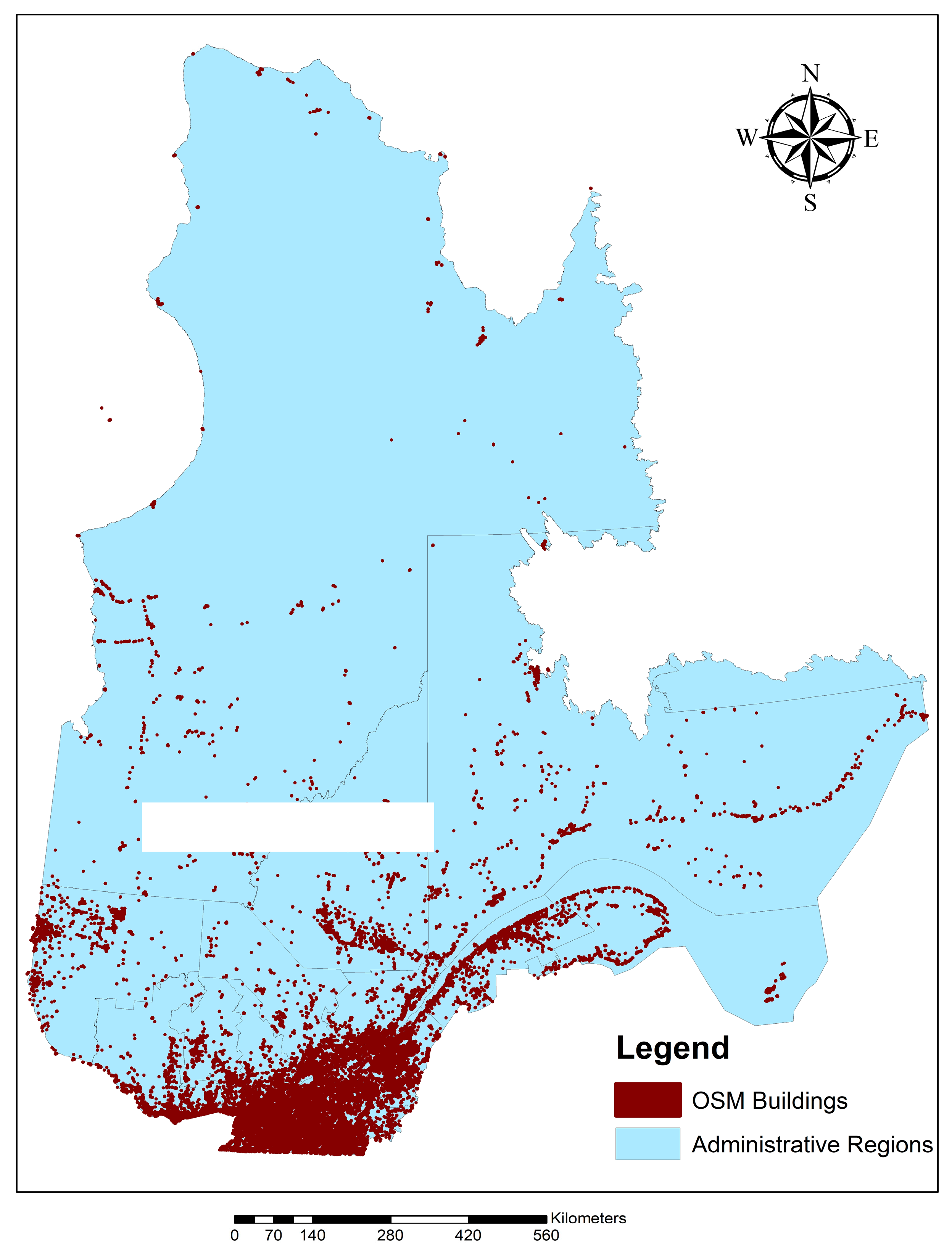
For this study, the OSM database for the province of Québec was retrieved on two distinct dates: 4 November 2018, and 1 October 2023, from GeoFabrik. This dataset encompasses building footprints across the province. Consequently, the specific study areas (the selected cities) needed to be extracted from the entire database. Figure 2 displays the spatial distribution of building footprints within the province in 2023.

As Figure 2 demonstrates, there is a higher density of building footprints in the southern region of the province. Because reference data are not available for all areas, the OSM building footprint dataset must be clipped to the city boundaries to ensure consistent borders between both datasets. On 4 November 2018, the OSM database contained 311,465 buildings for the Québec province, covering a total area of 173,743,179.59 square meters. The average building area was 557.8 square meters, with the smallest and largest footprint areas being 0.0033 square meters and 228,942.6 square meters, respectively.

2.9. Preprocessing

In the case of this research, preprocessing is required because the two datasets are not in the same projection systems. The database of OSM is in GCS_WGS_1984, while the reference data are in NAD83. Thus, both datasets should be projected in the same projection system to be able to continue the processes. NAD_1983_MTQ_Lambert is used in this research because it is designed to fit the road network of the Québec province.

In addition, both 2018 and 2023 OSM building data should be clipped with the boundary of the cities in order to have two equivalent datasets with the reference dataset. Figure 3 shows the reference data and clipped 2018 OSM data in Québec City.

The next step of preprocessing is removing the polygons that are smaller than 40 m² because they are most likely not representing buildings. Given that the majority of the building footprints in OSM are created by digitizing the areal images, it is likely that a parking or swimming pool is categorized as a building due to the low resolution of the Bing map aerial images.

2.10. Finding Corresponding Features

Feature matching is performed using the method proposed by Moradi et al. [36] for both 2018 and 2023 OSM datasets. To assess the precision of feature matching, the outcomes of the 2023 OSM data matched against reference data were subject to manual verification. For this purpose, 100 buildings were randomly selected from the reference dataset, and their corresponding structures in the 2023 OSM data were identified manually. The authors then ascertained the correspondence types for these 100 buildings. It was found that the correspondence type for only 2 out of the 100 buildings had been incorrectly assigned by the algorithm.

Once the correspondence types between the two datasets were established, comparisons of the paired polygons were conducted. This enables the evaluation of the completeness, positional accuracy, shape accuracy, and attribute accuracy of the OSM building footprints.

3. Results

3.1. Evaluating the Completeness

The completeness of the five cities was calculated using both area-based and object-based methods in 2018 and again in 2023.

3.1.1. Area-Based Completeness Evaluation

Two measures of completeness are calculated: based on the number of buildings in the two databases and based on the total area of the buildings in the two databases.

Table 2. The area-based completeness for the selected cities in the Québec province.

	City	Repentigny	Québec	Shawinigan	Rouyn-Noranda	Longueuil
OSM 2018	No. of Buildings	1693	14,409	384	421	3027
	Area (m2)	1,183,340	10,479,443	828,649	400,208	3,865,171
OSM 2023	No. of Buildings	9260	44,021	18,925	1370	8034
	Area (m2)	2,436,737	16,133,074	3,777,721	801,392	6,099,164
Reference Dataset	No. of Buildings	24,133	160,485	19,115	26,686	61,304
	Area (m2)	4,527,833	30,849,277	3,806,090	3,664,484	10,622,880
Completeness 2018	Based on Number	7%	9%	2%	1.5%	5%
	Based on Area	26%	34%	22%	11%	36%
	Ratio	3.7	3.7	11	7.3	7.2
Completeness 2023	Based on Number	38%	27%	99%	5%	13%
	Based on Area	53%	52%	99%	21%	57%
	Ratio	1.4	1.9	1	4.2	4.3

shows the area-based completeness of the cities.

Table 2 indicates that in 2018, Québec City had the highest completeness rate among the five cities, while Rouyn-Noranda, the smallest of the selected cities, had the lowest completeness at only 1.5%. Additionally, there was a marked increase in the completeness of Shawinigan from 2018 to 2023. This variability reinforces the notion that OSM data quality is heterogeneous and that different cities—even those in proximity—cannot be presumed to have the same level of data quality.

This theory is further examined by analyzing the average building area in all cities according to OSM data.

Table 3. The average area of the building footprints in OSM and in the reference databases.

ID	City	Avg. Area in OSM (m2)		Avg. Area in Reference (m2)	Ratio
		2018	2023		2018	2023
1	Repentigny	698	263	187	3.7	1.4
2	Québec	727	366	192	3.7	1.9
3	Shawinigan	2157	204	199	10.8	1
4	Rouyn-Noranda	950	584	137	6.9	4.2
5	Longueuil	1276	759	173	7.3	4.3

presents the average area of building footprints for both the reference and OSM databases for 2018 and 2023. The data in Table 3 suggest that in nearly all cities, the average building area in OSM is significantly larger than that in the reference database, with the exception of Shawinigan in 2023. The variance between the area-based and number-based completeness measures could stem from the fact that OSM more comprehensively maps larger buildings, while smaller ones are often omitted.

The 2018 comparison between the cities also demonstrates that Québec and Longueuil tend to be slightly more complete than the other cities. Interestingly, by 2023, Shawinigan was nearly fully mapped.

Overall, the number-based measure of completeness improved for all cities in 2023. Québec City, Repentigny, Shawinigan, Rouyn-Noranda, and Longueuil experienced increases in completeness by 16%, 31%, 97%, 3.5%, and 8%, respectively.

3.1.2. Object-Based Completeness Evaluation

An object-based approach to completeness assessment is more reflective of reality, as it identifies corresponding features first before computing completeness based on the types of correspondence established. Thus, it allows for the quantification of completeness errors such as omissions and commissions.

Table 4. The object-based completeness assessment for the cities of the province of Québec.

ID	City	Omission (No. of B.)		Commission (No. of B.)		Completeness
		2018	2023	2018	2023	2018	2023
1	Repentigny	22,470	15,404	24	33	6.7%	35%
2	Québec	147,544	108,173	1164	1197	7.1%	24%
3	Shawinigan	18,840	288	138	159	1.05%	99%
4	Rouyn-Noranda	26,383	21,171	127	222	1.01%	4.5%
5	Longueuil	58,946	54,178	822	1168	3.2%	12%

presents the completeness of Québec cities using the object-based method.

Table 4 indicates that in 2023, there was an increase in commission values across all cities. This suggests that polygons representing new constructions or edifices, which were not included in previous authoritative datasets, have been incorporated by OSM contributors. On the flip side, the rate of omission errors declined in 2023, with Shawinigan showing a significant decrease. In Shawinigan, the addition of approximately 288 buildings would result in a 0% omission error rate, indicating the complete mapping of the city’s buildings.

3.2. Evaluating the Positional Accuracy

In this study, positional accuracy is determined by comparing the centroid of a polygon in OSM with the centroid of the reference polygon. The distance between these two centroids is measured and serves as the metric for positional accuracy. Thus, if an OSM building is digitized precisely at the same location as the reference building, the positional accuracy is considered high, and the distance between the centroids is zero. Conversely, a significant distance between the centroids indicates that the OSM building is far from its correct position, denoting low positional accuracy. Hence, there is an inverse relationship between positional accuracy and the centroid distance. Figure 4 displays the centroids of buildings in a sample area.

The mean distance between the two centroids is computed for each city, considering only the buildings that have a “1:1” relationship for this analysis. The positional accuracy of the building footprints is calculated using the PostGIS extension for the PostgreSQL database. Figure 5 shows the average distance between centroids for each city in the province of Québec for the years 2018 and 2023.

The positional accuracy of the building footprints is generally acceptable, considering that the quality of the aerial images is around 4 m. In 2018, the highest positional quality within the OSM database was observed for Repentigny, with a deviation of 2.1 m, and the lowest was for Shawinigan, with a deviation of 5.7 m. In Québec City, the average distance between the OSM centroid and the corresponding reference centroid was approximately 3.4 m, which is acceptable given the positional quality of the aerial images.

In 2023, the positional accuracy for all cities had improved, except for Repentigny, which experienced a minor decline of 0.1 m. This trend aligns with the authors’ expectations, as it is anticipated that the quality of OSM data will enhance over time due to increasing contributions (as per Linus’s law). Shawinigan underwent a significant improvement in positional accuracy, advancing from 5.7 m in 2018 to 1.1 m in 2023.

The distance between the two centroids provides information on the precision of the OSM polygon’s positioning relative to the corresponding Québec polygon. However, it does not reveal whether the building footprints are uniformly shifted in a particular direction or are scattered randomly. Therefore, this phase involves analyzing the scatter diagram of the displacements to determine if there is any discernible pattern. Figure 6 presents the scatter diagram of these displacements, which are calculated by comparing the position of the OSM building’s centroid to the reference building’s centroid. Figure 6 shows that in some cities, the displacement is not random. For instance, in Québec City, buildings are, on average, shifted toward the north and northeast, while in Rouyn-Noranda, the shift is toward the west and southwest. Additionally, the denser concentration of scatter points near the coordinate system’s center in 2023 compared to 2018 suggests an improvement in positional accuracy for Shawinigan.

To account for the shifts in the position of OSM buildings, the author postulates that the angle of the imagery and the satellite’s relative position to the city may cause some radial displacement of the building tops (which are the parts OSM contributors see and digitize, not the actual footprints). Buildings located farther from the image center may have rooftops that appear displaced from their footprints.

3.3. Evaluating the Shape Accuracy

As previously mentioned, the building footprints in OSM are primarily digitized by OSM contributors. Consequently, the shape of the digitized polygons does not exactly mirror the actual footprint shapes. This section will calculate five measures previously used in research to assess the shape accuracy of OSM building footprints in selected cities of the Québec province. These measures will provide insights into the resemblance of OSM building footprints to those in the reference database.

3.3.1. Calculating the Area Ratio

The area ratio, defined as the area of the building footprint in OSM relative to the area of the corresponding building in the reference database, is a basic yet informative measure of similarity between two polygons. This metric is straightforward to compute. Figure 7 depicts the area ratios of building footprints between the two databases.

According to Figure 7, the average area of buildings in OSM is comparable to the average area of the corresponding buildings in the reference database; the average ratio of the two areas is nearly 1 for all cities. The area ratio suggests that the shape accuracy of building footprints in Shawinigan within OSM has noticeably improved from 2018 to 2023. However, for most cities, this measure has remained stable. It is crucial to note that this area ratio is calculated exclusively for buildings that have a one-to-one correspondence with those in the reference database. Based on Figure 7, the area ratios of Rouyn-Noranda and Shawinigan are higher compared to those of the other cities. This suggests that the average area of OSM polygons relative to those in the reference database is larger in these cities. Consequently, it can be inferred that the shape accuracy of building footprints in Rouyn-Noranda and Shawinigan is lower. We hypothesize that the mapping quality in these two cities is inferior, as indicated by several quality measures being lower compared to other cities. A plausible explanation for this could be the lower population density in these areas.

3.3.2. Calculating Compactness

The similarity in compactness between the buildings in OSM and those in the reference database suggests a greater resemblance between them. While compactness does not reveal the exact degree of similarity between two sets of polygons, it offers insights into their comparative shapes. Figure 8 displays the compactness differences for the cities in 2018 and 2023.

Figure 8 indicates that, from 2018 to 2023, the compactness of OSM buildings has become more aligned with that of the reference database buildings across all cities, particularly in Shawinigan. The area ratio and compactness assess the general shape of the building footprint, providing an overarching notion of similarity. In contrast, the Hausdorff distance and average distance yield more detailed information about shape accuracy.

3.3.3. Calculating the Hausdorff Distance

The Hausdorff distance is a metric that quantifies how closely the points of two polygons approximate each other. It is an extreme measure, indicating the greatest distance across the peripheries of two polygons. Therefore, the Hausdorff distance is particularly effective for identifying significant errors or inaccuracies in the digitization of building footprints. In this study, each OSM polygon is initially adjusted to be concentric with its corresponding reference polygon. Following this, the Hausdorff distance between the adjusted OSM polygon and the reference polygon is computed. Subsequently, we calculate the average of these distances for each city. A Hausdorff distance of zero would imply that the points of both polygons coincide, suggesting similar shapes. Conversely, a large Hausdorff distance denotes dissimilarity in shape. Figure 9 presents the average Hausdorff distance for each city.

As illustrated in Figure 9, nearly all cities exhibit a reduced Hausdorff distance in 2023 compared to 2018, with the exception of Repentigny. Given that the Hausdorff distance identifies larger errors, it can be inferred that the polygon shapes in Repentigny might have been digitized with less precision from 2018 to 2023. Shawinigan has seen the most significant enhancement in shape accuracy, while the Hausdorff distance for Rouyn-Noranda has not changed more than 0.5 m since 2018.

3.3.4. Calculating the Average Distance

The Hausdorff distance is influenced by the maximum distance between the corresponding points of two polygons, representing extreme errors rather than the average dissimilarity between two shapes. Therefore, in this section, we use the average distance method to gauge the similarity of two shapes. Initially, the OSM polygon is aligned to be concentric with the reference building polygon. Subsequently, we compute the average distance between the OSM polygon and the corresponding reference polygon. Figure 10 depicts the average value of this distance for each city.

Figure 10 indicates that Rouyn-Noranda has the highest average distance, while Repentigny has the lowest. This suggests that the shape accuracy in Repentigny is superior to that of other cities, whereas Rouyn-Noranda has the least shape accuracy. Moreover, it can be deduced that shape accuracy has improved in 2023, which aligns with Linus’s law. The average distance for all cities is less than 1 m, signifying that, on average, the points of the OSM footprint polygons are less than 1 m away from those in the reference dataset when the polygons are concentric.

3.4. Evaluating the Attribute Accuracy

In this step, we evaluate the attributes of OSM buildings that are stored as tags. The most important attribute, the building’s name, is assessed here. All attributes in OSM are stored as key = value pairs. TagInfo (https://taginfo.openstreetmap.org/ (accessed on 12 September 2023)) is a website providing the most frequent tags associated with a key [46]. It is a valuable resource for evaluating the variety of tags contributors have used to describe geographic locations.

In this section, we compare the names of OSM buildings with those in the reference database using the Levenshtein distance algorithm. This algorithm quantifies the number of deletions, insertions, and substitutions required to convert string A into string B [45]. Thus, a high Levenshtein distance value indicates low similarity between two strings, while a distance of 0 means that the strings are identical. We calculate the Levenshtein distance between the names of buildings in OSM and those in the reference database, with lower values indicating better attribute quality.

For our reference databases, only buildings in the cities of Rouyn-Noranda and Repentigny have named entries, permitting comparison only within these locales. In Repentigny, 238 buildings, and in Rouyn-Noranda, 113 buildings are named. Other buildings, even in the reference database, do not have names, which is reasonable, as only a small percentage of buildings are named in reality. The average Levenshtein distance for Repentigny and Rouyn-Noranda in 2018 was 2.4 and 3.3, respectively. This suggests that, on average, building names had two-to-three letter differences from their actual names. By 2023, the average Levenshtein distances for Repentigny and Rouyn-Noranda improved slightly to 1.9 and 2.6, respectively, indicating a modest enhancement in attribute accuracy. Several of these discrepancies are related to French accents on letters such as “è,” “é,” “à,” etc. This issue arises partly because individuals do not always spell building names correctly. Users of OSM data in Québec should be mindful of this, as it can lead to challenges depending on the application in which the OSM data are employed.

4. Conclusions

This research evaluates the quality of OpenStreetMap (OSM) building footprint data between 2018 and 2023 in five selected cities—Québec City, Repentigny, Shawinigan, Rouyn-Noranda, and Longueuil—within the Québec province. The primary aim is to assess the current quality of OSM data and analyze how it has evolved over the past five years. Due to limited access to authoritative datasets, this study focuses on four key spatial data quality aspects: completeness, positional accuracy, attribute accuracy, and shape accuracy.

The findings indicate an overall improvement in data quality. Completeness, measured via object-based and area-based methods, showed significant progress. In 2018, the average area-based completeness across the cities was 25.8%, which increased to 56.4% by 2023. Similarly, the object-based completeness rose from 3.8% in 2018 to 34.9% in 2023, highlighting the active contributions made to the OSM project during this period. A noteworthy enhancement was seen in Shawinigan, where object-based completeness surged from 1% to 99%, illustrating the heterogeneous nature of OSM data quality. Positional accuracy also improved, with the average distance between the centroids of OSM and reference data decreasing from 3.7 m in 2018 to 2.3 m in 2023. This indicates that in the research area, the average distance between the centroids of OSM buildings and those of the reference buildings decreased by 1.4 m. This reduction may be attributed to the fact that subsequent modifications corrected positional errors in the buildings over the study period.

For shape accuracy, four metrics were evaluated: area ratio, compactness, Hausdorff distance, and average distance. While the area ratio and compactness provided broad shape information, they could not detect minor discrepancies. In contrast, the Hausdorff distance and average distance were more effective in differentiating the shape similarities and dissimilarities. The results showed a decrease in the average distance measure (in five cities) and suggested an improvement in the shape accuracy overall. Moreover, the average distance measure was less than 1 m for all cities in both 2018 and 2023, which means that all building footprints of the province have a relatively good shape accuracy. In addition, the Hausdorff distance value indicates a reduction in the number of major errors in the shape of buildings over the study period.

Attribute accuracy, assessed using the Levenshtein distance for building names, indicated minimal discrepancies, typically not exceeding two-to-three characters in both 2018 and 2023. Our study’s findings suggest a minor but noteworthy improvement in the attribute accuracy of OpenStreetMap (OSM) building names over the course of our research period.

We were constrained in expanding our research to other cities and villages of the province due to the lack of access to recent, consistent, and high-quality reference datasets. Another limitation relates to the outdated nature of the available data: the reference data only represent buildings as of 2018. Consequently, new constructions and modifications in the buildings post-2018, which could slightly alter the calculated measures, are not accounted for in our research. This aspect presents an opportunity for future researchers to explore the temporal quality of OSM in greater detail. Additionally, exploring the relationship between the quality of OSM data and the rate of improvement of OSM data over time, in relation to variables such as population, income, and other potential quality indicators, could be a fascinating topic for future studies.

Additionally, the study observed that incomplete cities in OSM have larger average building footprints compared to reference data, leading to the hypothesis that contributors may prioritize digitizing larger buildings. This hypothesis, proposing that the average size of OSM buildings could serve as an indicator of completeness in areas lacking reference data, can be explored in future research. Future research could extend beyond the building name to other OSM building attributes, further enriching our understanding of data quality and contributing to the enhancement of OSM data.