1. Introduction
Understanding and monitoring eruptive events through the analysis of volcanic activity images play a pivotal role in prompt hazard assessment, especially at open-vent volcanoes that frequently erupt, such as Mount Etna in Italy [
1,
2,
3]. The proliferation of visual data from remote sensors, drones, and spatial-based techniques demands advanced methodologies for extracting detailed information. Neural networks, particularly Convolutional Neural Networks (CNNs), have emerged as powerful tools for image analysis, being capable of learning complex patterns and spatial relationships. However, classifying volcanic images poses unique challenges due to the diverse and dynamic nature of volcanic phenomena. This is particularly difficult when considering the gradual transition from one eruptive activity to another, or when the same eruptive class exhibits peculiar behaviors.
This study delved into thermal image classification, focusing on applying CNNs to distinguish various states of Mount Etna. The volcano’s activity is monitored using a variety of geophysical sensors, including thermal cameras installed on the ground [
1] or on special satellites [
2].
Thermal image classification is a common application of machine learning algorithms, with some immune-based machine learning algorithms demonstrating efficacy in this regard, as highlighted in [
4,
5,
6,
7]. However, while immune-based machine learning algorithms offer valuable reference points, our study focused on evaluating the effectiveness of pretrained Convolutional Neural Networks (CNNs) in addressing the classification problem within the context of volcanic activity monitoring. This research contributes to the early detection and assessment of eruptive events, facilitating timely responses for hazard mitigation and risk management. Furthermore, our study underscores the importance of transfer learning. By considering pretrained neural networks and retraining them with a limited dataset specific to volcanic activity, we demonstrate the practical effectiveness of transfer learning in environmental monitoring applications.
A valuable application of CNNs to detect subtle to intense anomalies exploiting the spatial relationships of volcanic features on a labeled dataset of ASTER TIR images from five different volcanoes, namely, Etna (Italy), Popocatepetl (Mexico), Lascar (Chile), Fuego (Guatemala), and Klyuchevskoy (Russia), was proposed by [
3]. The detection and segmentation of volcanic ash plumes using the segNet and U-Net CNN architectures at Mt. Etna was proposed by [
8]. The classification of video observation data for volcanic activity on Klyuchevskoy Volcano by using neural networks was also proposed by [
9].
Traditionally, training a CNN for image classification involves random weight initialization and optimization on a specific dataset. However, the advent of pretrained CNN models on large image datasets provides new opportunities for applying knowledge acquired from other domains, as highlighted by [
10], who achieved a remarkable overall accuracy of
in recognizing eruptive activity from satellite images at seven different volcanoes. The authors developed a monitoring system aimed at automatically detecting thermal anomalies associated with volcanic eruptions across different volcanoes worldwide, including locations such as La Palma (Spain), Etna (Italy), and Kilauea (Hawaii, USA). The study primarily focused on leveraging the pretrained SqueezeNet model to discern high-temperature volcanic features in thermal infrared satellite data. This approach significantly reduces training time by fine-tuning the model with a novel dataset comprising both thermal anomalies and non-anomalous volcanic features. The training dataset was crafted with two classes, one containing volcanic thermal anomalies (erupting volcanoes) and the other containing no thermal anomalies (non-erupting volcanoes), to differentiate between volcanic scenes with eruptive and non-eruptive activity. Satellite imagery acquired via ESA Sentinel-2 MSI and NASA and USGS Landsat 8 OLI/TIRS instruments, specifically in the infrared bands, served as the primary data source for analysis.
In this study, we considered various popular pretrained CNNs to classify images acquired by the INGV-OE (Istituto Nazionale di Geofisica e Vulcanologia, Osservatorio Etneo) thermal camera network, classifying the eruptive states of Mount Etna into six categories. Video files of Mount Etna activity are recorded by fixed, continuously operating thermal cameras on the volcano’s flanks, transmitting real-time images to the INGV-OE Operative Room. Operators aim to recognize eruptive events promptly, especially any sudden changes in the volcano’s state, emphasizing, once more, the importance of the accurate classification of eruptive activity.
2. Material and Methods
Of the five units comprising the network of thermal cameras monitoring Etna’s activity (EMOT, ESR, EMCT, EBT, and ENT), we considered all the images recorded by the EMOT camera. This decision was based on the potential variations in classification arising from different locations and cameras simultaneously capturing images, as highlighted by [
2]. It is worth noting that training a classifier for each camera is necessary when considering images from more than one camera.
For details regarding the geographical coordinates and technical features of the individual cameras installed on Etna, interested readers can refer to the paper [
2].
The dataset analyzed in this study consisted of 476 images extracted from the original
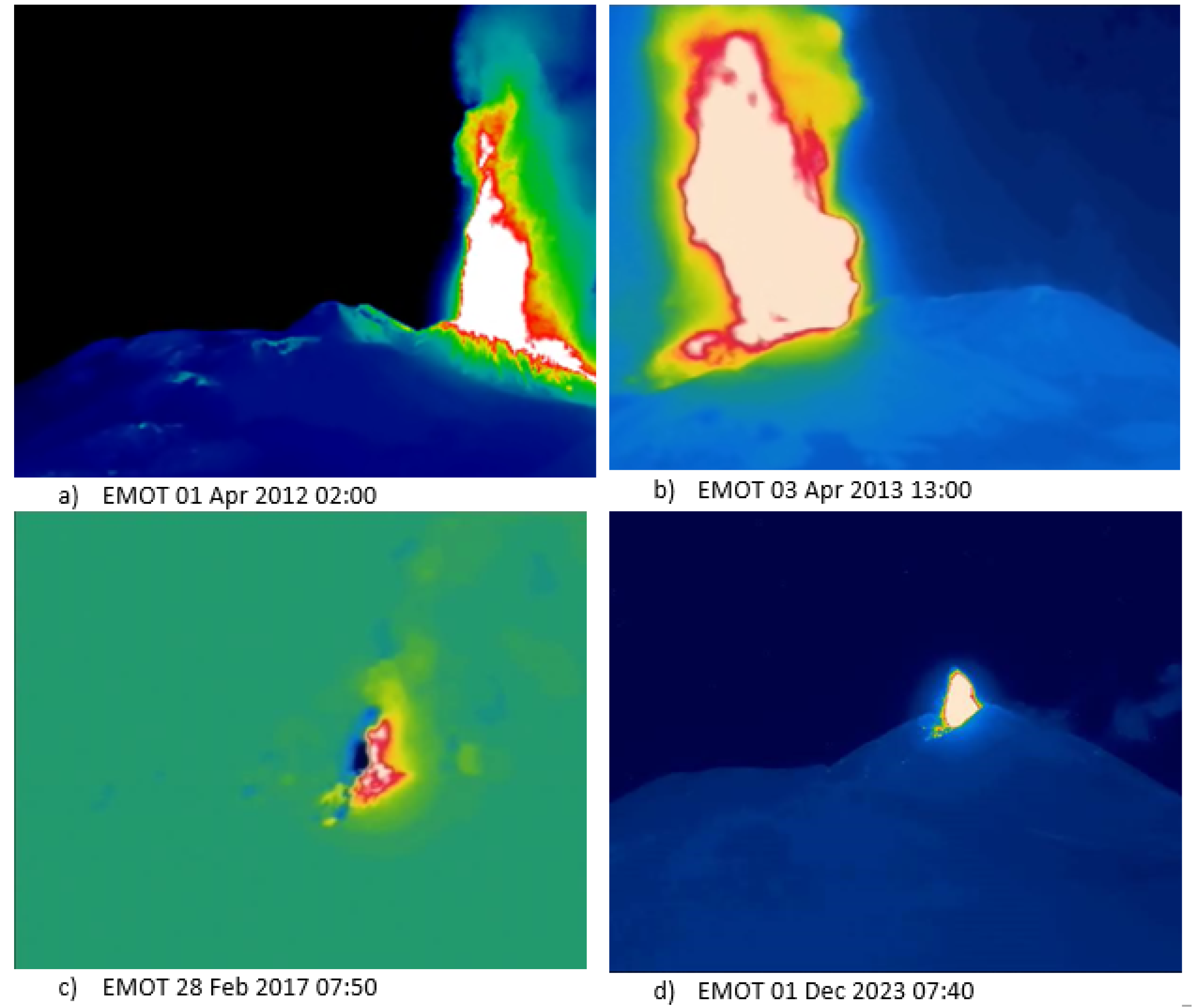
.avi files in [481, 601, 3] RGB format, recorded between 2011 and 2023. These images were labeled into six classes: (1) No activity, (2) Strombolian, (3) Lava Fountain, (4) Lava flow or cooling spatter, (5) Degassing or ash emission, and (6) Cloudy. Typical images belonging to these classes are shown in
Figure 1. The images were organized into a Matlab datastore. A short description of the considered classes is provided below:
- Class 1
No activity:
- Class 2
Strombolian:
Strombolian activity is a type of mildly explosive volcanic activity. From a geophysical perspective, Strombolian activity is characterized by a medium amplitude of seismic tremor, a shallower source of seismic tremor, the presence of clustered infrasonic events, no eruption column or ash emissions, and discrete bursts with an ejection of hot material. However, geophysical signals are not relevant for classifying activity from images, which is instead based on the low height of the ejected matter and on the pulsating behavior typical of Strombolian activity.
- Class 3
Lava Fountain:
Characteristics associated with Lava Fountain eruptions include a high amplitude of seismic tremor RMS (Root Mean Square), the presence of clustered infrasonic events, and a shallower source of seismic tremor. However, these features are not relevant for classifying activity from images, which is instead based on the steady ejection of spatter at a medium or high height.
- Class 4
Lava flow or cooling products (spatter, flow, or tephra):
This class refers to volcanic activity related to the output of lava flow or to the cooling of previously erupted lava, spatter, or tephra, forming a static hot deposit slowly cooling down. It may involve the movement of molten rock on the Earth’s surface or the solidification of previously erupted lava or pyroclastic material.
- Class 5
Degassing or ash emission:
Degassing is a volcanic process involving the release of hot gases, such as water vapor, carbon dioxide, sulfur dioxide, and/or little dilute ash, from the summit craters of a volcano. The emitted ash forms a transparent plume, easily distinguished from the thick and dense ash plume formed during Lava Fountains (Class 3). This activity may occur without significant eruptive events. Dilute ash emissions can be released during small bursts or even intra-crater landslides.
- Class 6
Cloudy:
It should be noted that these classes are not mutually exclusive for obvious reasons due to the possibility of intermediate types of activity between classes. For example, if an image exhibits Lava Fountain activity, it may also feature gas or ash emission, possibly accompanied by clouds, as shown in
Figure 2. Additionally, since the summit of Etna comprises four active craters, it is possible for them to erupt simultaneously, exhibiting different behaviors, although such events are rare but not impossible [
11]. In such cases, we expect the classifier to report the class to which the image predominantly belongs.
One of the challenges in classifying images of volcanic activity arises from the inherent complexities introduced by environmental factors, even when captured by fixed cameras. The dynamic nature of volcanic landscapes, combined with diverse atmospheric conditions and varying insolation, contributes to the difficulty of achieving accurate and consistent classification results. In
Figure 2, various images attributed to the Lava Fountain class are presented to highlight the variability.
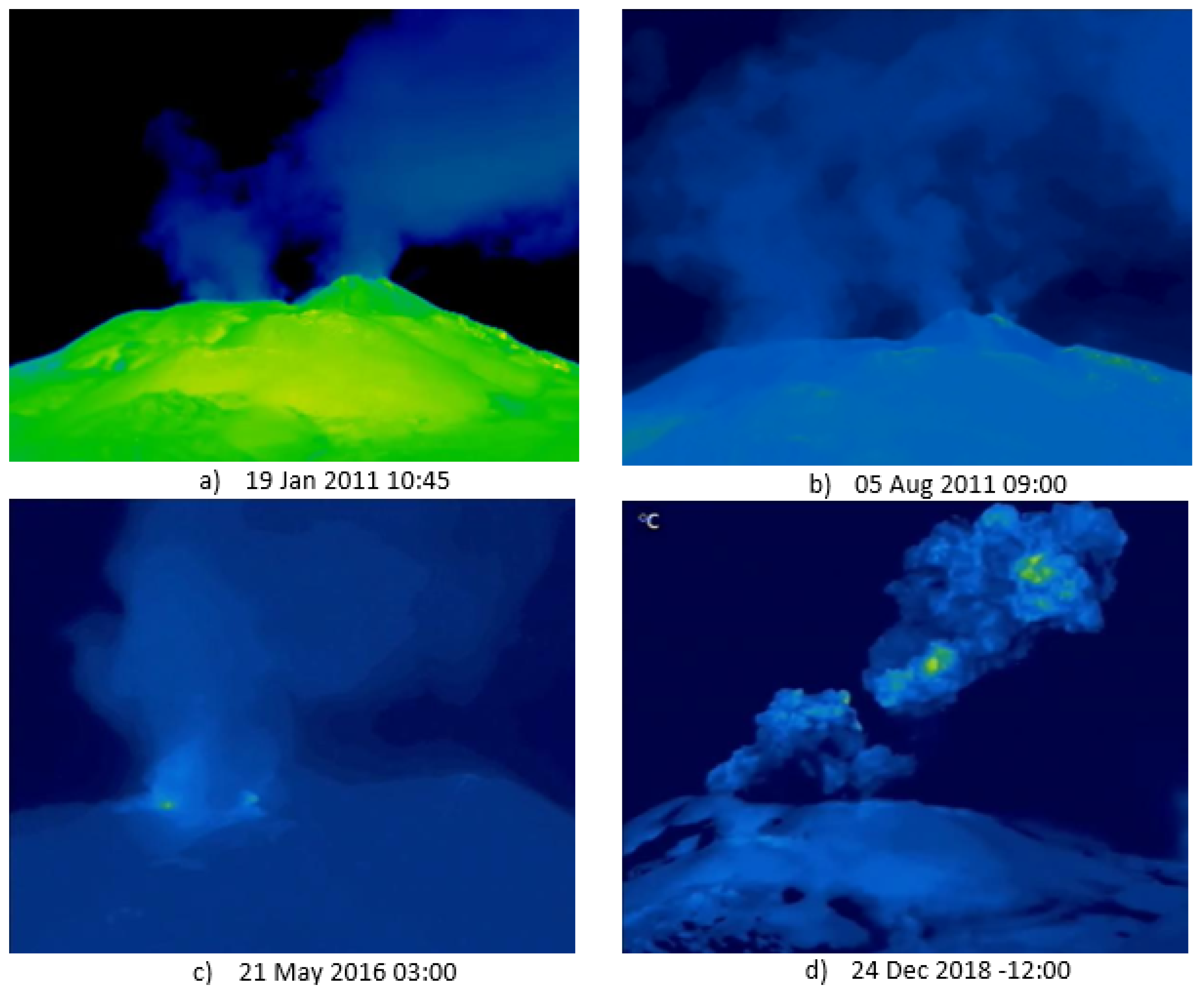
Similarly, degassing or ash emission can vary significantly, as illustrated in
Figure 3.
This problem applies to all the other classes considered, and for brevity and space, they are not extensively shown. In summary, fixed cameras, while providing continuous surveillance, are susceptible to disturbances stemming from changing lighting conditions throughout the day and night.
In addition to the challenges posed by lighting and thermal considerations, images of volcanic areas are also significantly impacted by the unpredictable and highly variable meteorological conditions inherent in volcanic regions. The interplay of these elements introduces additional sources of noise and variability, making it challenging to develop a one-size-fits-all classification model. To tackle these difficulties, we opted to utilize Convolutional Neural Networks (CNNs), given their proven effectiveness in handling complex classification tasks under diverse conditions, as demonstrated by their performance in competitions like the one described by [
12].
2.1. Overview of CNN Architecture
This section provides an overview of the fundamental components that constitute the architecture of a CNN, avoiding detailed discussions that interested readers can find in specific papers [
13,
14] and/or textbooks [
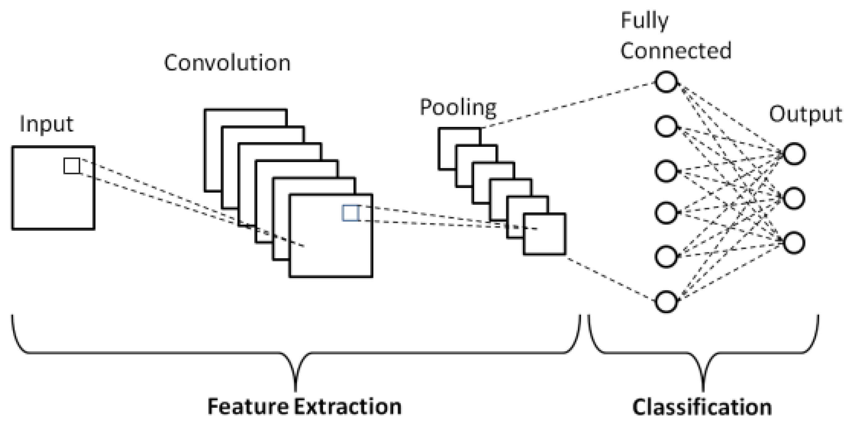
15]. In contrast to traditional neural networks, CNNs are specifically designed to efficiently handle grid-like data, such as images. Broadly speaking, a CNN consists of three different kinds of layers: Convolutional Layers, Pooling Layers, and Fully Connected Layers, as schematically shown in
Figure 4.
The cornerstone of CNNs is the convolutional layers. These layers apply convolution operations to input data using filters or kernels, enabling the network to capture spatial hierarchies and learn local patterns. The convolutional operation involves sliding the filter across the input, performing element-wise multiplications, and aggregating the results to create feature maps.
Pooling layers are essential for reducing the spatial dimensions of the input volume, thereby decreasing the computational complexity of the network. Common techniques like max pooling and average pooling downsample feature maps, retaining the most important information while discarding less relevant details. The last layer of the CNN is the output layer, producing the final predictions. The choice of activation function in this layer depends on the nature of the task, such as softmax for classification problems or linear activation for regression tasks.
2.2. Pretrained vs. Non Pretrained CNN
Pretrained Convolutional Neural Networks (CNNs) are trained on large datasets such as ImageNet [
12], learning hierarchical features useful for a wide range of computer vision tasks. Leveraging a pretrained CNN for a specific task brings the advantage of utilizing these learned features, known as transfer learning. Advantages include the following:
Feature Transfer: Early layers of a CNN learn basic features like edges and textures, which are relatively generic and transfer well to various tasks.
Efficient Training: Training a CNN from scratch requires substantial labeled data and computational resources. Pretrained models, trained on large datasets only require an adjustment of the final layers for specific tasks.
Performance Boost: Using a pretrained model can lead to better performance, especially when a limited amount of data is available.
The pretrained networks considered in this study are listed in
Table 1, along with their topological features (extracted from [
16]).
Here is a brief description of the considered models:
SqueezeNet: A lightweight neural network architecture designed for efficient model inference with a relatively small number of parameters [
17].
GoogleNet: Also known as Inception v1 [
18], introduced the inception module, which enables the network to capture features at multiple scales. It is known for its deep architecture and efficient use of parameters.
DenseNet201: The Dense Convolutional Network connects each layer to every other layer in a feed-forward fashion [
19]. DenseNet201 specifically has 201 layers and is known for its parameter efficiency.
ResNet18: The Residual Network introduced residual connections to address the vanishing gradient problem [
20]. ResNet18 has 18 layers and has been widely used in various computer vision tasks.
ShuffleNet: Designed for efficient channel shuffling and parameter reduction [
21]. It is known for its ability to achieve a good accuracy with fewer parameters.
DarkNet19: The neural network framework behind the YOLO (You Only Look Once) object detection system. Darknet19 has 19 layers [
22].
AlexNet: A pioneering Convolutional Neural Network architecture that gained prominence for winning the ImageNet Large Scale Visual Recognition Challenge in 2012 [
23]. It consists of five convolutional layers and three fully connected layers.
VGG-16: VGG (Visual Geometry Group) architectures are known for their simplicity and uniformity. VGG-16 has 16 layers, consisting of small 3 × 3 convolutional filters [
24].
For further details, interested readers can refer to [
14] and references therein, and/or to the Matlab Deep Learning Toolbox [
16].
3. Experimental Setup and Evaluation Metrics
The software development environment used for the classification of the images in this work was Matlab. In this framework, pretrained CNN models could be imported. To prepare for the retraining of these networks, RGB images from the datastore, originally of size [481, 601, 3], were resized according to the dimensions expected by each network (see the Input Dimension column in
Table 1 [
16]). Additionally, for each network, the classification layer was modified to accommodate the number of classes considered in this application, i.e., 6.
Images from the datastore were randomly divided into a training set and a validation set, with equal proportions. The optional training parameters, such as activation functions, mini-batch size, and initial learning rate, were kept the same for all the CNNs considered. For each network, training was halted when the accuracy had visually reached a plateau, and there was no longer appreciable improvement. At the conclusion of the training, accuracy was calculated on the validation set. The classifier accuracy was assessed as described in the following section, Section Evaluation Metrics.
Evaluation Metrics
In a classification experiment, let
and
denote the number of actual positive and actual negative cases in the
i-th class, respectively. Moreover, let
,
,
, and
represent the number of true positive, true negative, false positive, and false negative cases, respectively, recognized by the classifier, for the
i-th class. Based on these quantities, the following rates can be defined:
These indices can be interpreted as follows:
expresses the proportion of actual positives correctly classified by the model as belonging to the i-th class. The best values of TPR approach 1, while the worst case is when TPR approaches 0. is also known as Recall or Sensitivity.
expresses the proportion of actual negatives correctly classified as not belonging to the i-th class. Similar to , the best values of TNR approach 1, while the worst values approach 0. is also known as Specificity.
expresses the proportion of false negatives in the i-th class, with respect to all actual positives in the same class. In the best case, approaches 0, while in the worst case, it approaches 1.
expresses the proportion of false positives in the i-th class with respect to the total number of actual negatives in the same class. Similar to , in the best case, approaches 0, while in the worst case, it approaches 1.
Another useful index is the Positive Predicted Value (
PPV) or
Precision, which, for the generic class
i, is defined as
Here,
stands for False Discovery Rate. A useful way to collect most of these performance indices is the Confusion Matrix (CM), examples of which are shown in
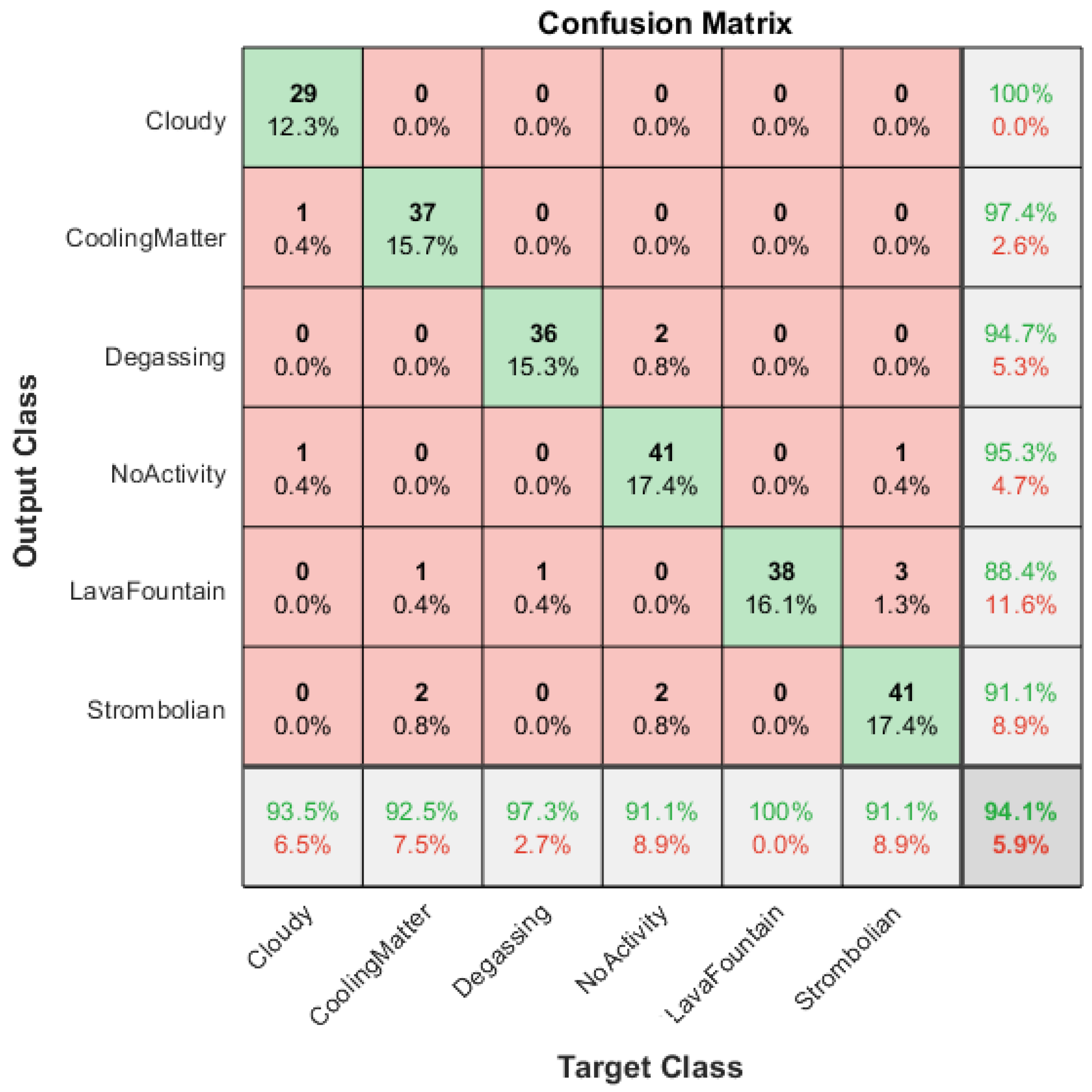
Section 4. On the confusion matrix (CM), the rows correspond to the predicted class (Output Class), and the columns correspond to the true class (Target Class). The diagonal cells correspond to correctly classified observations, while the off-diagonal cells correspond to incorrectly classified observations. Both the number of observations and the percentage of the total number of observations are shown in each cell. The column on the far right of the plot shows the percentages of all the examples predicted to belong to each class that are correctly and incorrectly classified, i.e., the
and the
. The row at the bottom of the plot shows the percentages of all the examples belonging to each class that are correctly and incorrectly classified, i.e., the
TPR(
i) and the
, respectively. The cell in the bottom right of the plot shows the total accuracy, here referred to as
totAcc. The total accuracy can formally be described by using expression (
6):
where
is a function that returns 1 if g is true and 0 otherwise,
is the class label assigned by the classifier to the sample ,
is the true class label of the sample ,
N is the number of samples in the testing set.
If expression (
6) refers to the individual classes, i.e., evaluating expression (
7)
where
is the number of samples in class i in the testing set,
K is the total number of classes,
We obtain the classical rate. However, in this paper, we prefer to use the term class accuracy instead of and refer to it as .
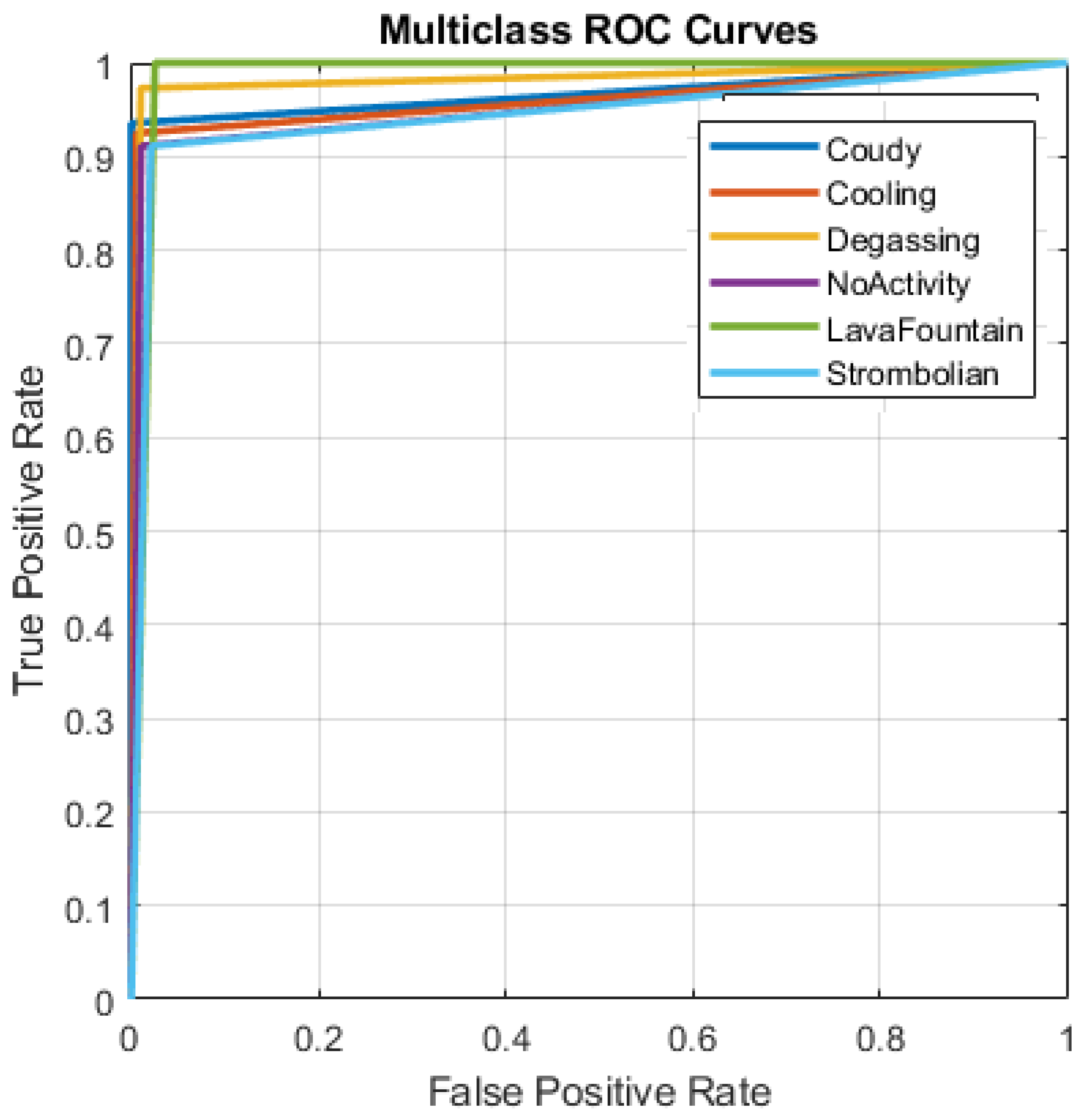
Another useful tool for evaluating the reliability of supervised classifiers is the Receiver Operating Characteristic (ROC) metric and, in particular, the area under curve (AuC(i)), where the i-th index refers to the class. The ROC curves typically feature the true positive rate on the Y axis and the false positive rate on the X axis. The top-left corner of the plot is the ideal point, characterized by a false positive rate of zero and a true positive rate of one. The best values of approach 1, while for a classifier performing randomly, approaches 0.5.
4. Numerical Results
In this section, we provide a comprehensive analysis of the performance of various neural networks employed for the classification of volcanic activity images in the considered case study. The primary evaluation focuses on the crucial metric of total accuracy, providing a holistic measure of each network’s ability to correctly classify images across all classes.
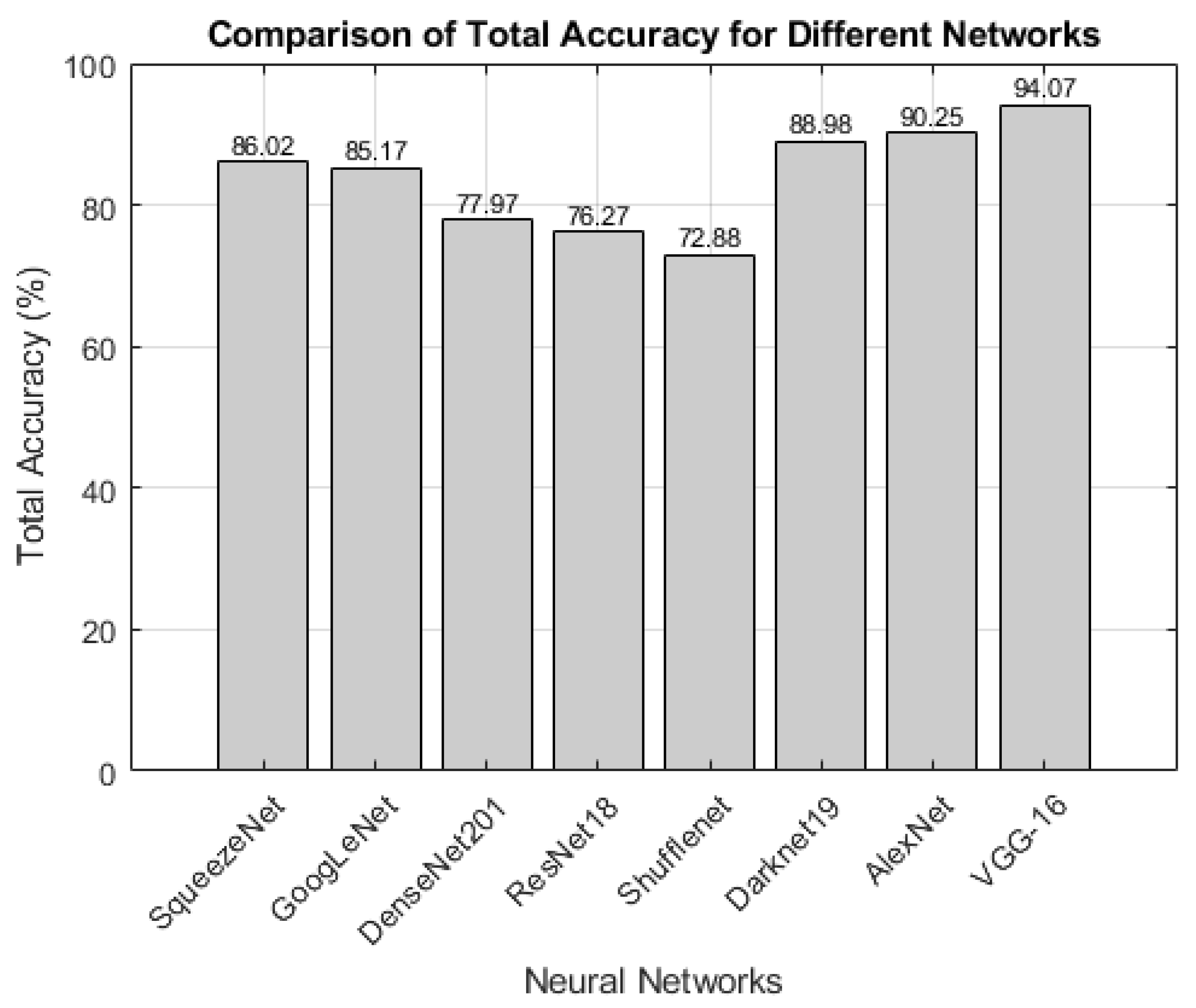
Figure 5 illustrates the total accuracy achieved by different neural networks, each trained and tested as described in the previous
Section 3. The total accuracy values represent the percentage of correctly classified instances across all classes. Therefore, a higher total accuracy indicates a more robust and effective network for the given classification task.
Based on the total accuracy, it appears that VGG-16 and AlexNet exhibited a total accuracy greater than , with VGG-16 outperforming the others considered in the comparison, exhibiting a total accuracy of about .
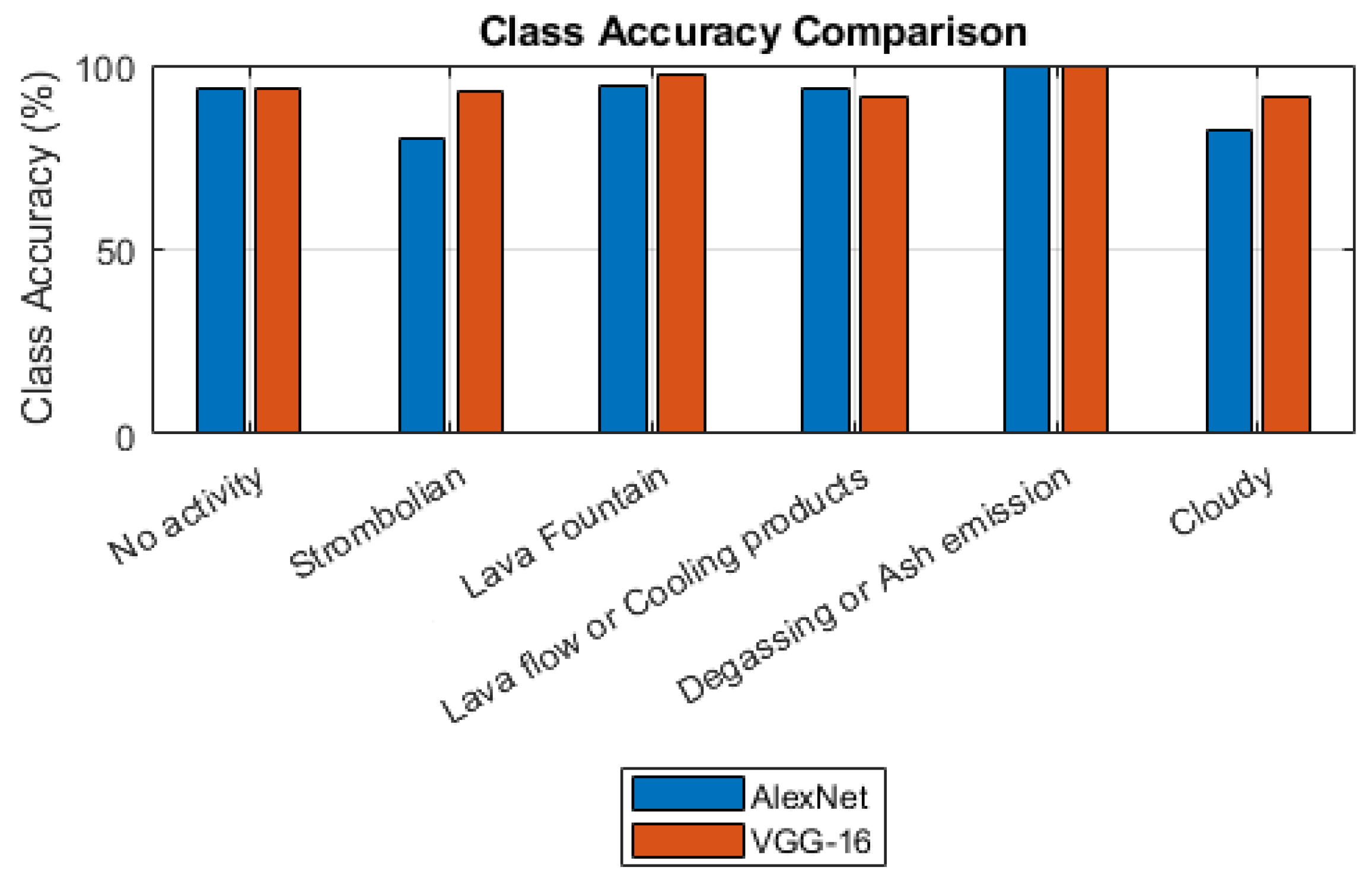
For deeper insights, the class accuracies for the VGG-16 and AlexNet CNN pretrained models are shown in
Figure 6.
It is seen that the two classifiers had a similar accuracy with reference to the “No activity”, “Lava flow or cooling products”, and “Degassing or ash emission” classes, with a slight superiority of VGG-16 for the remaining classes (“Strombolian”, “Lava Fountain”, and “Cloudy”).
The performances of VGG-16 in terms of the Confusion Matrix and ROC curves are shown in
Figure 7 and
Figure 8, respectively.
It is necessary to stress that the two networks that exhibited the greatest accuracy, VGG-16 and AlexNet, are the ones with the greatest number of parameters, as shown in
Table 1. Specifically, VGG-16 and AlexNet have 138 million and 61 million parameters, respectively. Therefore, the cost of their higher accuracy compared to the others could be attributed to this feature, which makes the learning phase slower and requires greater computational resources. However, we believe that these aspects are less decisive in the choice of the model, since once trained, the classifier can be implemented on standard computers available in a monitoring room. It is necessary to observe that images are recorded with a frame rate of 1 or 2 frames per second, depending on the considered camera, which is much lower than the classification time, typically a few milliseconds. However, at the present stage of the project, the re-training of a classifier cannot be performed online since, for a large model like VGG-16 and our dataset of images, it takes about 30 min to complete the training phase.
Highlighting the Role of Transfer Learning
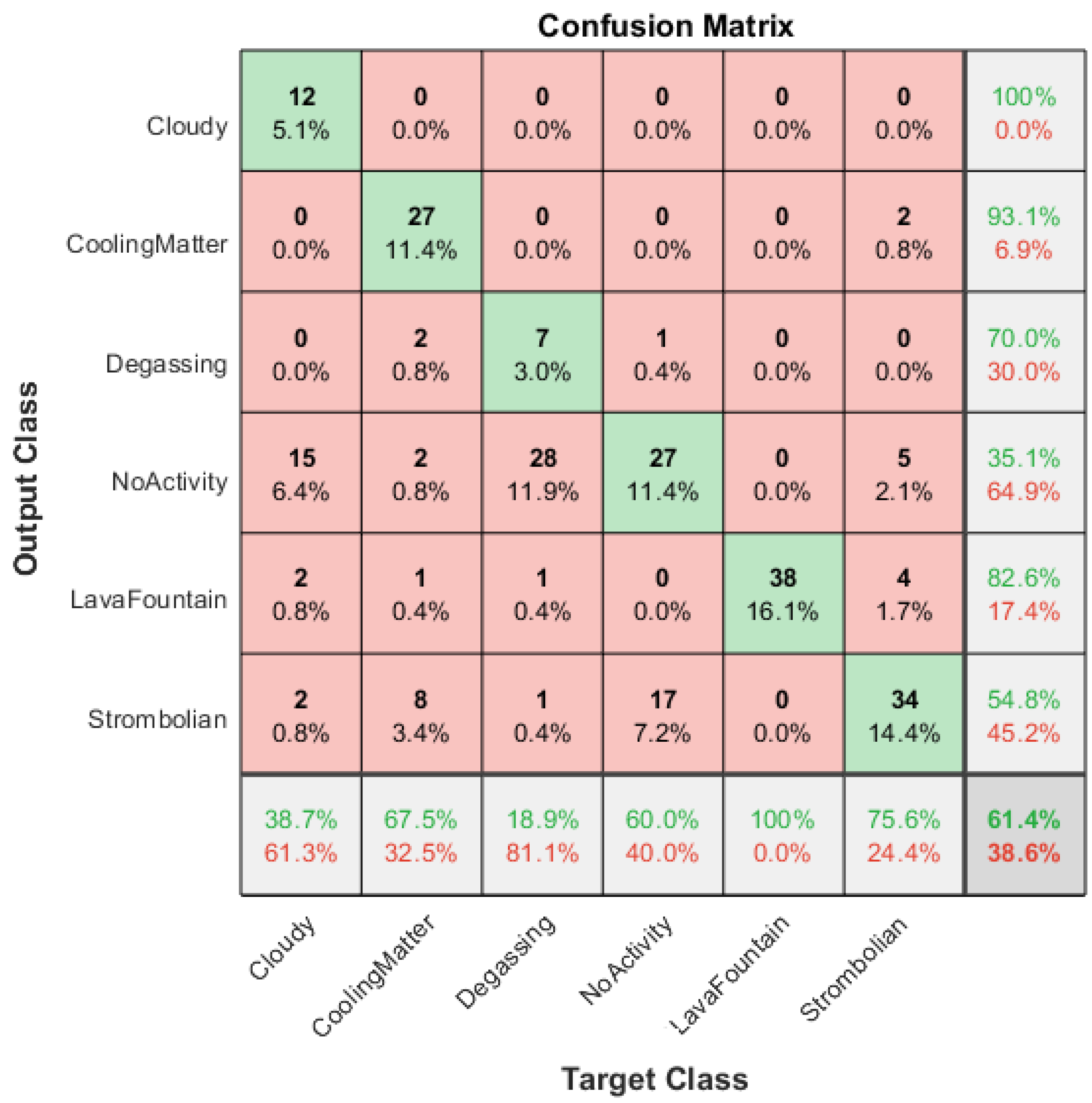
To assess the impact of transfer learning, we implemented the following strategy. Having established that the classification of volcanic activity images into six classes can be achieved with satisfactory accuracy using a pretrained VGG-16, we attempted to train a network with an identical architecture as VGG-16, but with randomly initialized connection weights. We only adjusted the number of output classes to six. The non-pretrained network was then trained using the same options employed for training the pretrained VGG-16 model.
Upon the completion of the training, the network achieved results summarized by the confusion matrix reported in
Figure 9.
As it is possible to see, the total accuracy achieved was . Notably, only the images belonging to the Lava Fountain class were correctly classified (class accuracy ), and with a lower accuracy, images of the Strombolian class (class accuracy ). Images belonging to the remaining classes were poorly classified.
Additionally, we considered a custom CNN with 17 layers, including 5 convolution layers and 302,374 parameters. This custom CNN exhibited the following performance metrics: total accuracy of , which is evidently insufficient.
The stark contrast in performance between the pretrained networks and the networks trained from scratch underscores the effectiveness of transfer learning for the considered application. The pretrained VGG-16, leveraging knowledge from a broader dataset, outperformed the networks initialized without pretrained weights. Transfer learning not only improved the overall accuracy but also demonstrated the capability to recognize a diverse set of volcanic activity classes.
5. Conclusions
This study addresses the challenging task of classifying thermal images capturing the eruptive activity of Mount Etna, leveraging Convolutional Neural Networks (CNNs) with a focus on pretrained models. Eight widely recognized pretrained neural networks were rigorously experimented, demonstrating their efficacy in solving the classification problem for ground-based thermal camera imagery.
Through empirical testing, several pretrained networks proved effective in achieving an impressive total accuracy of approximately after retraining on a limited dataset of 476 images. Notable performers included VGG-16, AlexNet, DarkNet201, GoogleNet, and SqueezeNet.
A crucial finding of this work is the significance of transfer learning. Attempting to solve the classification problem without leveraging pretrained networks yielded unsatisfactory results, highlighting the effectiveness of transfer learning in geospatial imagery analysis, especially in scenarios with limited labeled data.
In conclusion, the work conducted thus far is considered a work in progress, with a series of planned extensions. Efforts are underway to expand the dataset of images used for training from the current 476 to encompass thousands. However, this endeavor is time-consuming and labor-intensive, given the meticulous process of data collection, labeling, and verification required. The aim is not only to include data from a single camera, as demonstrated in this study, but also ideally from all cameras within the network.
Furthermore, it is essential to develop an effective strategy for distinguishing strong Strombolian activity from light Lava Fountain activity in the images. Currently, this distinction relies more on volcanologists’ experience than measurable geometric factors, presenting an ongoing challenge that requires careful consideration.
In summary, the results presented here provide significant impetus to continue towards the adoption of pretrained classifiers for an effective solution to the problem posed in this work.
Author Contributions
Conceptualization, G.N. and S.C.; methodology, G.N.; software, G.N.; validation, G.N. and S.C.; formal analysis, G.N. and S.C.; investigation, G.N. and S.C.; resources, G.N. and S.C.; data curation, G.N. and S.C.; writing—original draft preparation, G.N. and S.C.; writing—review and editing, G.N. and S.C.; visualization, G.N. and S.C.; supervision, G.N. and S.C.; project administration, G.N.; funding acquisition, G.N. and S.C. All authors have read and agreed to the published version of the manuscript.
Funding
Supported by Italian Research Center on High Performance Computing Big Data and Quantum Computing (ICSC), project funded by European Union—NextGenerationEU—and National Recovery and Resilience Plan (NRRP)—Mission 4 Component 2 within the activities of Spoke 3 (Astrophysics and Cosmos Observations). Sonia Calvari also acknowledges the financial support of the Project FIRST ForecastIng eRuptive activity at Stromboli volcano (Delibera n. 144/2020; Scientific Responsibility: S.C.) Vulcani 2019.
Data Availability Statement
Images considered in this paper were extracted from videos of an eruptive activity paper belonging to the Istituto Nazionale di Geofisica e Vulcanologia, Osservatorio Etneo Sezione di Catania. Selected images can be made available upon request to Dr Sonia Calvari of the INGV-OE.
Acknowledgments
We would like to thank the INGV-OE scientists and technicians for the monitoring network maintenance, and especially Michele Prestifilippo for providing information essential for this work.
Conflicts of Interest
The authors declare no conflicts of interest.
References
- Calvari, S.; Nunnari, G. Comparison between automated and manual detection of lava fountains from fixed monitoring thermal cameras at Etna volcano, Italy. Remote Sens. 2022, 14, 2392. [Google Scholar] [CrossRef]
- Corradino, C.; Ganci, G.; Cappello, A.; Bilotta, G.; Herault, A.; Del Negro, C. Mapping recent lava flows at Mount Etna using multispectral Sentinel-2 images and machine learning techniques. Remote Sens. 2019, 11, 1916. [Google Scholar] [CrossRef]
- Corradino, C.; Ramsey, M.S.; Pailot-Bonnetat, S.; Harris, A.J.L.; Del Negro, C. Detection of subtle thermal anomalies: Deep learning applied to the ASTER Global Volcano Dataset. IEEE Trans. Geosci. Remote Sens. 2023, 61, 1–15. [Google Scholar] [CrossRef]
- Yu, X.; Zhou, Z.; Gao, Q.; Li, D.; Riha, K. Infrared Image Segmentation Using Growing Immune Field and Clone Threshold. Infrared Phys. Technol. 2017, 88, 184–193. [Google Scholar] [CrossRef]
- Yu, X.; Lu, Y.; Gao, Q. Pipeline image diagnosis algorithm based on neural immune ensemble learning. Int. J. Press. Vessel. Pip. 2021, 189, 104249. [Google Scholar] [CrossRef]
- Yu, X.; Ye, X.; Zhang, S. Floating pollutant image target extraction algorithm based on immune extremum region. Digit. Signal Process. 2022, 123, 103442. [Google Scholar] [CrossRef]
- Velesaca, H.O.; Bastidas, G.; Rohuani, M.; Sappa, A.D. Multimodal image registration techniques: A comprehensive survey. Multimed. Tools Appl. 2024. [Google Scholar] [CrossRef]
- Guerrero Tello, J.F.; Coltelli, M.; Marsella, M.; Celauro, A.; Palenzuela Baena, J.A. Convolutional neural network algorithms for semantic segmentation of volcanic ash plumes using visible camera imagery. Remote Sens. 2022, 14, 4477. [Google Scholar] [CrossRef]
- Korolev, S.; Sorokin, A.; Urmanov, I.; Kamaev, A.; Girina, O. Classification of video observation data for volcanic activity monitoring using computer vision and modern neural networks (on Klyuchevskoy volcano example). Remote Sens. 2021, 13, 4747. [Google Scholar] [CrossRef]
- Amato, E.; Corradino, C.; Torrisi, F.; Del Negro, C. A deep convolutional neural network for detecting volcanic thermal anomalies from satellite images. Remote Sens. 2023, 15, 3718. [Google Scholar] [CrossRef]
- Calvari, S.; Cannavó, F.; Bonaccorso, A.; Spampinato, L.; Pellegrino, A.G. Paroxysmal Explosions, Lava Fountains and Ash Plumes at Etna Volcano: Eruptive Processes and Hazard Implications. Front. Earth Sci. 2018, 6, 107. [Google Scholar] [CrossRef]
- Russakovsky, O.; Deng, J.; Su, H.; Krause, J.; Satheesh, S.; Ma, S.; Huang, Z.; Karpathy, A.; Khosla, A.; Bernstein, M.; et al. ImageNet Large Scale Visual Recognition Challenge. Int. J. Comput. Vis. 2015, 115, 211–252. [Google Scholar] [CrossRef]
- Alzubaidi, L.; Zhang, J.; Humaidi, A.J.; Al-Dujaili, A.; Duan, Y.; Al-Shamma, O.; Santamaría, J.; Fadhel, M.A.; Al-Amidie, M.; Farhan, L. Review of deep learning: Concepts, CNN architectures, challenges, applications, future directions. J. Big Data 2021, 8, 53. [Google Scholar] [CrossRef] [PubMed]
- Taye, M.M. Theoretical Understanding of Convolutional Neural Network: Concepts, Architectures, Applications, Future Directions. Computation 2023, 11, 52. [Google Scholar] [CrossRef]
- Goodfellow, I.; Bengio, Y.; Courville, A. Deep Learning; MIT Press: Cambridge, MA, USA, 2016. [Google Scholar]
- MathWorks. MATLAB Deep Learning Toolbox. 2022. Available online: https://www.mathworks.com/products/deep-learning.html (accessed on 20 February 2024).
- Iandola, F.N.; Han, S.; Moskewicz, M.W.; Ashraf, K.; Dally, W.J.; Keutzer, K. SqueezeNet: AlexNet-level accuracy with 50× fewer parameters and <0.5 MB model size. Sensors 2016, 16, 94. [Google Scholar] [CrossRef]
- Szegedy, C.; Liu, W.; Jia, Y.; Sermanet, P.; Reed, S.; Anguelov, D.; Erhan, D.; Vanhoucke, V.; Rabinovich, A. Going Deeper with Convolutions. In Proceedings of the 2015 IEEE Conference on Computer Vision and Pattern Recognition (CVPR), Boston, MA, USA, 7–12 June 2015. [Google Scholar] [CrossRef]
- Wang, S.H.; Zhang, Y.D. DenseNet-201-Based Deep Neural Network with Composite Learning Factor and Precomputation for Multiple Sclerosis Classification. Acm Trans. Multimed. Comput. Commun. Appl. 2020, 16, 60. [Google Scholar] [CrossRef]
- He, K.; Zhang, X.; Ren, S.; Sun, J. Deep residual learning for image recognition. In Proceedings of the 2016 IEEE Conference on Computer Vision and Pattern Recognition (CVPR), Las Vegas, NV, USA, 27–30 June 2016; pp. 770–778. [Google Scholar]
- Zhang, X.; Zhou, X.; Lin, M.; Sun, J. ShuffleNet- An Extremely Efficient Convolutional Neural Network for Mobile Devices. Sensors 2017, 17, 874. [Google Scholar] [CrossRef]
- AhmadChoudhry, Z.; Shahid, H.; Naqvi, S.Z.H.; Aziz, S.; Khan, M.U. DarkNet-19 based Decision Algorithm for the Diagnosis of Ophthalmic Disorders. In Proceedings of the 2021 International Conference on Innovative Computing (ICIC), Lahore, Pakistan, 9–10 November 2021; pp. 1–6. [Google Scholar] [CrossRef]
- Krizhevsky, A.; Sutskever, I.; Hinton, G.E. ImageNet Classification with Deep Convolutional Neural Networks. In Advances in Neural Information Processing Systems; Pereira, F., Burges, C.J., Bottou, L., Weinberger, K.Q., Eds.; Curran Associates, Inc.: New York, NY, USA, 2012; Volume 25, Available online: https://proceedings.neurips.cc/paper_files/paper/2012/file/c399862d3b9d6b76c8436e924a68c45b-Paper.pdf (accessed on 20 February 2024).
- Simonyan, K.; Zisserman, A. Very Deep Convolutional Networks for Large-Scale Image Recognition. arXiv 2015, arXiv:1409.1556. [Google Scholar]
| Disclaimer/Publisher’s Note: The statements, opinions and data contained in all publications are solely those of the individual author(s) and contributor(s) and not of MDPI and/or the editor(s). MDPI and/or the editor(s) disclaim responsibility for any injury to people or property resulting from any ideas, methods, instructions or products referred to in the content. |
© 2024 by the authors. Licensee MDPI, Basel, Switzerland. This article is an open access article distributed under the terms and conditions of the Creative Commons Attribution (CC BY) license (https://creativecommons.org/licenses/by/4.0/).


