Roles of Earth’s Albedo Variations and Top-of-the-Atmosphere Energy Imbalance in Recent Warming: New Insights from Satellite and Surface Observations

Abstract

Past studies have reported a decreasing planetary albedo and an increasing absorption of solar radiation by Earth since the early 1980s, and especially since 2000. This should have contributed to the observed surface warming. However, the magnitude of such solar contribution is presently unknown, and the question of whether or not an enhanced uptake of shortwave energy by the planet represents positive feedback to an initial warming induced by rising greenhouse-gas concentrations has not conclusively been answered. The IPCC 6th Assessment Report also did not properly assess this issue. Here, we quantify the effect of the observed albedo decrease on Earth’s Global Surface Air Temperature (GSAT) since 2000 using measurements by the Clouds and the Earth’s Radiant Energy System (CERES) project and a novel climate-sensitivity model derived from independent NASA planetary data by employing objective rules of calculus. Our analysis revealed that the observed decrease of planetary albedo along with reported variations of the Total Solar Irradiance (TSI) explain 100% of the global warming trend and 83% of the GSAT interannual variability as documented by six satellite- and ground-based monitoring systems over the past 24 years. Changes in Earth’s cloud albedo emerged as the dominant driver of GSAT, while TSI only played a marginal role. The new climate sensitivity model also helped us analyze the physical nature of the Earth’s Energy Imbalance (EEI) calculated as a difference between absorbed shortwave and outgoing longwave radiation at the top of the atmosphere. Observations and model calculations revealed that EEI results from a quasi-adiabatic attenuation of surface energy fluxes traveling through a field of decreasing air pressure with altitude. In other words, the adiabatic dissipation of thermal kinetic energy in ascending air parcels gives rise to an apparent EEI, which does not represent “heat trapping” by increasing atmospheric greenhouse gases as currently assumed. We provide numerical evidence that the observed EEI has been misinterpreted as a source of energy gain by the Earth system on multidecadal time scales.

1. Introduction

The 6th Assessment Report of the Intergovernmental Panel on Climate Change (IPCC AR6) concluded “It is very likely that well-mixed GHGs [greenhouse gases] were the main driver of tropospheric warming since 1979” [1] (p. 5). This statement implies that all known climate forcings have properly been evaluated using the available data, and GHGs have been found to exert a disproportionally large radiative effect on the Global Surface Air Temperature (GSAT) over the past 45 years. However, a close examination of Chapter 7 of the Working Group I (WG1) Contribution to the IPCC AR6 [2], which discusses the Earth’s energy budget, climate feedbacks and climate sensitivity, reveals that the observed decrease of Earth’s albedo and the corresponding increase of absorbed shortwave radiation by the planet for the past 20 years have not been taken into account as a contributor to the recent warming. Section 7.2.2 of Chapter 7 entitled “Changes in Earth’s Energy Budget” acknowledges that there have been multidecadal periods of significant decreasing and increasing trends in surface solar radiation (SSR) called “global dimming” (i.e., from the 1950s to the 1980s) and “global brightening” (after 1980s), respectively. The Report states: “There is high confidence that these [SSR] trends are widespread, and not localized phenomena or measurement artefacts”. Indeed, the existence of such dimming and brightening periods has been acknowledged by researchers for more than 10 years [3,4]. However, the IPCC AR6 provides no global estimate about the magnitude of the positive SSR trend since the 1980s and its significance for the observed increase in GSAT. The Report ends a discussion about SSR variations by stating “The origin of these trends is not fully understood”. With respect to the Top-of-the-Atmosphere (TOA) solar fluxes, Section 7.2.2 offers no analysis of the substantial decrease in Earth’s shortwave reflectance observed since 2000 and documented by the NASA’s Clouds and the Earth’s Radiant Energy System (CERES) project [5,6,7,8]. The Report does not mention the 2.0 W m⁻² increase in solar-energy uptake by the planet from 2000 to 2020 and its effect on GSAT. Even more surprisingly, Section 7.2.2.1 of the IPCC WG1 Contribution features two graphs in their Figure 7.3 (on p. 936) showing a positive trend in the Earth’s reflected solar radiation and a negative trend in the outgoing thermal flux since 2000 that are supposedly based on CERES data. However, these trends are the opposite of what CERES has actually measured and contradict prior published results.

A number of studies have analyzed the CERES data and concluded that the observed increase of shortwave-radiation absorption by Earth likely played a dominant role in driving global warming over the past 2 decades [5,8,9,10]. However, to our knowledge, no study has yet quantified the amount of warming attributable to solar forcing alone, i.e., the increase of GSAT due to Earth’s decreasing albedo combined with a varying Total Solar Irradiance (TSI). Without such a quantitative assessment, the amount of warming attributed to rising atmospheric greenhouse gases remains a theoretical speculation.

We attempted to fill this knowledge gap by embarking on a “follow-the-energy” journey aimed at quantifying the specific contribution of solar forcing to the GSAT increase from March 2000 through December 2023. To accomplish this, we applied a new, generic model (derived from independent NASA planetary data using objective rules of calculus) to TOA radiative-flux anomalies measured by CERES. The model explicitly links changes of GSAT to variations in TSI and planetary Bond albedo. Since the model equations are developed without relying on Earth-specific data, they are applicable to any spherical celestial body with a rocky surface. By comparing the Earth’s observed GSAT evolution to that predicted by the model, we were able to separate the impact of solar drivers from the anthropogenic forcing of climate. The model also helped obtain important new insights about the physical nature of the Earth Energy Imbalance (EEI), which is currently viewed as the most important indicator for climate change.

2. Data and Methods

2.1. Satellite and Surface Datasets

The data utilized in this study are globally averaged, monthly time series of TOA radiative fluxes, lower-troposphere (near-surface) temperatures, and 0–100 m depth ocean temperatures. We used shortwave and longwave radiative fluxes measured by the CERES project and their deseasonalized anomalies, along with GSAT anomalies provided by seven datasets based on satellite and ground monitoring platforms. Globally averaged temperature anomalies of the top 100 m oceanic layer were obtained from the latest version of the gridded dataset of ocean subsurface temperatures provided by the Institute of Atmospheric Physics (IAP) at the Chinese Academy of Sciences [11].

Table 1. Datasets utilized in this study. URLs accessed on 19 August 2024.

Dataset Name & Version (Reported Parameters)	Monitoring Platform	World Wide Web URL
CERES EBAF 4.2 (TOA Radiative Fluxes)	Satellite	https://ceres-tool.larc.nasa.gov/ord-tool/jsp/EBAFTOA42Selection.jsp
HadCRUT5 (GSAT)	Surface Sensors	https://hadleyserver.metoffice.gov.uk/hadcrut5/data/HadCRUT.5.0.2.0/download.html
NOAA GlobalTemp (GSAT)	Surface Sensors	https://www.ncei.noaa.gov/access/monitoring/climate-at-a-glance/global/time-series
NASA GISTEMP 4.0 (GSAT)	Surface Sensors	https://data.giss.nasa.gov/gistemp/tabledata_v4/GLB.Ts+dSST.txt
BEST, Berkeley Earth Surface Temperature (GSAT)	Surface Sensors	https://berkeley-earth-temperature.s3.us-west-1.amazonaws.com/Global/Land_and_Ocean_complete.txt
NOAA STAR MSU/AMSU-A/ATMS 5.0 (Lower Troposphere Temperature)	Satellite	https://www.star.nesdis.noaa.gov/smcd/emb/mscat/products.php
RSS 4.0 (Lower Troposphere Temperature)	Satellite	https://data.remss.com/msu/monthly_time_series/RSS_Monthly_MSU_AMSU_Channel_TLT_Anomalies_Land_and_Ocean_v04_0.txt
UAH 6.0 (Lower Troposphere Temperature)	Satellite	https://www.nsstc.uah.edu/data/msu/v6.0/tlt/uahncdc_lt_6.0.txt
IAP 4.0 Global, gridded dataset of ocean subsurface temperatures. (Ocean Temperatures)	Underwater Sensors	http://www.ocean.iap.ac.cn/pages/dataService/dataService.html?navAnchor=dataService

lists all datasets and their versions used in this study, along with valid URLs for data downloading as of 19 August 2024.

Since our intent was to study the climate behavior on annual and longer time scales, the timeseries of monthly anomalies were smoothed by computing 13-month running means for each series. All data analyses presented here were performed on smoothed monthly anomalies in this way. For the sake of simplicity, our analysis only utilized the central (best) estimate of each dataset, as suggested by the official data custodians. We do not discuss the uncertainty of individual datasets here, because these have been documented in the references and download URLs provided.

Figure 1 shows examples of raw and smoothed anomalies of the Earth’s global albedo and shortwave radiation absorption over the period March 2000–December 2023, inferred from the CERES Energy-Balanced and Filled (EBAF) 4.2 dataset. Figure 2 depicts monthly TSI anomalies computed from CERES monthly measurements of shortwave insolation. Note that TSI exhibits a nearly zero trend over the past 24 years, and its fluctuations (±0.48 W m⁻²) represent only a fraction of the observed changes in the absorbed shortwave flux depicted in Figure 1b. According to CERES observations, the Earth’s all-sky albedo has declined by approximately 0.79% since 2000 causing an increase of planetary shortwave radiation absorption of ≈2.7 W m⁻². For comparison, the IPCC AR6 estimated a total anthropogenic forcing of 2.72 W m⁻² driving climate change from 1750 to 2019 [2] (Section 7.3.5.2). Thus, the solar forcing measured over the past 2.4 decades has the same magnitude as the total anthropogenic forcing estimated by models for the past 27 decades. This fact further stresses the urgency to quantify the contribution of observed albedo changes to the recent planetary warming.

Figure 3 depicts GSAT 13-month running mean anomalies of the temperature datasets listed in Table 1 over the 24-year observational period of CERES. Although differences among individual datasets are small in terms of GSAT variation patterns, we found that UAH reported an anomalously low rate of warming since 2000 compared to all other datasets (Figure 4). This made UAH an outlier in our assessment and led to a decision to remove it from the analysis. The GSAT monthly anomalies of the remaining six datasets (i.e., HadCRUT5, GISTEMP4, NOAA GlobalTemp, BEST, RSS and NOAA STAR) were averaged to produce a representative temperature series for the Earth from 1981 through 2023, which was subsequently smoothed using a 13-month running mean to yield an annual temperature record suitable for our analysis. Figure 5 illustrates the result from this statistical procedure. The final time series indicates that the rate of planetary warming was significantly higher during the 21st Century compared to prior decades.

To assess the contribution of observed changes in TSI and planetary albedo to the increase of Earth’s GSAT, we employed a new model that explicitly relates global temperature responses to solar forcing and was derived by applying rules of calculus to a prior published universal planetary temperature model based on independent NASA data from rocky planets and moons in our Solar System [12]. The new climate-sensitivity model was run with CERES radiative flux data (i.e., anomalies of TSI and planetary albedo) to generate expected global temperature changes and a warming trend, which were then compared to the actual observed GSAT anomalies and trend over the period 2000–2023. All measured and model-generated data discussed here are available as Supplementary Material in a self-explanatory Microsoft Excel file accompanying this publication.

2.2. Modeling the Response of Global Surface Air Temperature to Solar Forcing

Nikolov and Zeller [12] developed a semiempirical mathematical model by applying Dimensional Analysis to vetted NASA planetary observations that accurately describes the long-term (baseline) average global surface temperature ($T_b$, K) of rocky planets and moons throughout the Solar System using only two forcing variables: the TOA mean annual TSI ($S$, W m⁻²) and the mean surface total atmospheric pressure ($P$, Pa), i.e.:

$$T_b=A S^{0.25} E_a\left(P\right)$$

(1)

In this equation, $A$ is a proportionality coefficient with units of K/(W m⁻²)^0.25 inferred from a generic analytical formula for calculating the average surface temperature of airless planetary bodies derived by Volokin and ReLlez [13] via spherical integration of the Stephan–Boltzmann radiation law, and $E_a\left(P\right)$ is the Relative Atmospheric Thermal Effect/Enhancement (RATE), which is a dimensionless, nonlinear function of $P$. The product $A{S}^{0.25}$ defines the global surface temperature of a planetary body (K) in the absence of atmosphere, while $E_a\left(P\right)$ accounts for the adiabatic enhancement of the no-atmosphere temperature due to the force of air pressure. The dependence of RATE on pressure shown in Figure 6 was empirically quantified using non-linear regression analysis of measured NASA data from 6 rocky planets and moons spanning a broad range of physical conditions in the Solar System. We will not discuss the functional form of $E_a\left(P\right)$ here, since it is not relevant to the present analysis and has been explained elsewhere [12]. Although technically speaking $A$ is not a constant (as it depends on the magnitude of a planet’s average geothermal flux heating the surface), it is nevertheless a conservative quantity with a narrow range of variation in the Solar System ($32.44\le A\le 33.68$). For Earth, $A=32.51$ K/(W m⁻²)^0.25.

Since Equation (1) accurately reproduces the long-term mean absolute GSAT of rocky planets and moons over a broad range of atmospheric and radiative environments (i.e., from Venus to Pluto), it can be differentiated to derive universal analytical formulas for calculating the response of a planetary GSAT to various forcing agents.

Assuming that GSAT variations are caused by simultaneous changes in TSI ($S$), planetary albedo ($\alpha$, fraction), and mean surface pressure ($P$), one can write the total differential of the global temperature as follows:

$$dT=\left({\displaystyle \frac{𝜕T}{𝜕S}}\right)dS+\left({\displaystyle \frac{𝜕T}{𝜕\alpha }}\right)d\alpha +\left({\displaystyle \frac{𝜕T}{𝜕P}}\right)dP$$

(2)

Since the surface air pressure does not change on time scales of decades to centuries (i.e., $dP=0$), one can ignore the last term on the right-hand side of Equation (2). Thus, the total change of GSAT (${\mathsf{\Delta }T}_t$, K) can be written in a finite-difference form as:

$${\mathsf{\Delta }T}_t={\mathsf{\Delta }T}_s+{\mathsf{\Delta }T}_{\alpha }$$

(3)

where ${\mathsf{\Delta }T}_s$ and ${\mathsf{\Delta }T}_{\alpha }$ are the temperature contributions due to TSI and albedo variations, respectively. One can derive analytical expressions for ${\mathsf{\Delta }T}_s$ and ${\mathsf{\Delta }T}_{\alpha }$ by applying the chain rule of calculus to Equation (1).

Thus, the total derivative of GSAT with respect to TSI is given by:

$${\displaystyle \frac{dT}{dS}}={\displaystyle \frac{𝜕T}{𝜕S}}+{\displaystyle \frac{𝜕T}{𝜕P}}{\displaystyle \frac{𝜕P}{𝜕S}}$$

(4)

Since, in the absence of large orbital shifts, the surface atmospheric pressure is independent of TSI, one can safely assume $𝜕P/𝜕S=0$. This eliminates the second term on the right-hand side of Equation (4). Equation (1) yields the following GSAT derivative with respect to TSI:

$${\displaystyle \frac{dT}{dS}}={\displaystyle \frac{1}{4}} A S^{0.25} E_a\left(P\right) {\displaystyle \frac{1}{S}}={\displaystyle \frac{T}{4 S}}$$

(5)

Upon separation of variables and integrating both sides of Equation (5), we get:

$${\int }_{T_b}^{T_b+\Delta {\mathit{T}}_{\mathit{s}}}{\displaystyle \frac{dT}{T}}={\displaystyle \frac{1}{4}}{\int }_{S_b}^{S_b+\mathsf{\Delta }s} {\displaystyle \frac{dS}{S}}$$

(6)

where $S_b$ is the baseline (average) TSI over the time period of interest (W m⁻²) and $\mathsf{\Delta }s$ is the TSI departure (anomaly) from $S_b$. The solution to Equation (6) is:

$$\ln \left({\displaystyle \frac{T_b+\mathsf{\Delta }{T}_s}{T_b}}\right)=\ln \left[{\left({\displaystyle \frac{S_b+\mathsf{\Delta }s}{S_b}}\right)}^{0.25}\right]$$

(7)

Taking the antilogarithm and solving for $\mathsf{\Delta }{T}_s$ yields:

$$\mathsf{\Delta }{T}_s= T_b\left[{\left(1+{\displaystyle \frac{\mathsf{\Delta }s}{S_b}}\right)}^{0.25}-1\right]$$

(8)

The total derivative of GSAT with respect to planetary albedo can be obtained by combining Equation (1) with a well-known formula relating the amount of absorbed shortwave radiation by a spherical body ($S_a$, W m⁻²) to TSI and its Bond albedo ($\alpha$), i.e.:

$$S_a={\displaystyle \frac{S}{4}}\left(1-\alpha \right)$$

(9)

Applying the chain rule of calculus, we get:

$${\displaystyle \frac{dT}{d\alpha }}={\displaystyle \frac{𝜕T}{𝜕S}}{\left({\displaystyle \frac{𝜕S_a}{𝜕S}}\right)}^{-1}{\displaystyle \frac{𝜕S_a}{𝜕\alpha }}+{\displaystyle \frac{𝜕T}{𝜕P}}{\displaystyle \frac{𝜕P}{𝜕\alpha }}$$

(10)

Again, since the surface atmospheric pressure has no dependency on the albedo (i.e., $𝜕P/𝜕\alpha =0$), the last term $\left({\displaystyle \frac{𝜕T}{𝜕P}}{\displaystyle \frac{𝜕P}{𝜕\alpha }}\right)$ in Equation (10) vanishes. From Equation (9), we obtain the partial derivatives:

$${\displaystyle \frac{𝜕S_a}{𝜕S}}={\displaystyle \frac{1-\alpha }{4}}$$

(11a)

$${\displaystyle \frac{𝜕S_a}{𝜕\alpha }}=-{\displaystyle \frac{S}{4}}$$

(11b)

Combining Equation (10) with Equations (5), (11a) and (11b) yields:

$${\displaystyle \frac{dT}{d\alpha }}=-{\displaystyle \frac{T}{4\left(1-\alpha \right)}}$$

(12)

Upon separation of variables and integrating both sides of Equation (12), we get:

$${\int }_{T_b}^{T_b+\mathsf{\Delta }{T}_{\alpha }}{\displaystyle \frac{dT}{T}}=-{\displaystyle \frac{1}{4}}{\int }_{{\alpha }_b}^{{\alpha }_b+\mathsf{\Delta }\alpha } {\displaystyle \frac{d\alpha }{1-\alpha }}$$

(13)

where ${\alpha }_b$ is the baseline (average) albedo over the time period of interest corresponding to a baseline absolute temperature $T_b$, and $\mathsf{\Delta }\alpha$ is the albedo departure (anomaly) from ${\alpha }_b$. The solution to Equation (13) is:

$$\ln \left({\displaystyle \frac{T_b+\mathsf{\Delta }{T}_{\alpha }}{T_b}}\right)=\ln \left[{\left({\displaystyle \frac{1-{\alpha }_b-\mathsf{\Delta }\alpha }{1-{\alpha }_b}}\right)}^{0.25}\right]$$

(14)

Taking the antilogarithm and solving for $\mathsf{\Delta }{T}_{\alpha }$ produces the final formula:

$$\mathsf{\Delta }{T}_{\alpha }=T_b\left[{\left(1-{\displaystyle \frac{\mathsf{\Delta }\alpha }{1-{\alpha }_b}}\right)}^{0.25}-1\right]$$

(15a)

Equation (15a) has an alternative form yielding equivalent results, which uses anomalies of the absorbed shortwave flux ($\mathsf{\Delta }{s}_a$) instead of albedo anomalies ($\mathsf{\Delta }\alpha$). It follows from Equation (11b) that $\mathsf{\Delta }\alpha =-\mathsf{\Delta }{s}_{a}4/S$, which, upon substitution into Equation (15a), yields a formula for calculating the change of GSAT ($\mathsf{\Delta }{T}_{sa}$) in response to a change in the absorbed solar flux:

$$\mathsf{\Delta }{T}_{sa}=T_b\left[{\left(1+{\displaystyle \frac{4 \mathsf{\Delta }{s}_a}{S(1-{\alpha }_b)}}\right)}^{0.25}-1\right]=\mathsf{\Delta }{T}_{\alpha }$$

(15b)

Combining Equations (3), (8) and (15a) produces an expression that quantifies the total response of GSAT to simultaneous changes of TSI ($\mathsf{\Delta }s$) and the planetary albedo ($\mathsf{\Delta }\alpha$):

$${\mathsf{\Delta }T}_t=T_b\left[{\left(1+{\displaystyle \frac{\mathsf{\Delta }s}{S_b}}\right)}^{0.25}+{\left(1-{\displaystyle \frac{\mathsf{\Delta }\alpha }{1-{\alpha }_b}}\right)}^{0.25}-2\right]$$

(16)

This formula has universal validity, since its derivation did not rely on Earth-specific data. Hence, it is applicable to any rocky planet and moon in the Solar System. Equation (16) implies that a planet’s climate sensitivity to solar forcing is proportional to the absolute baseline GSAT $T_b$ and increases nonlinearly with the baseline albedo, ${\alpha }_b$.

Since Equation (16) predicts the deviation of GSAT from a baseline temperature, $T_b$, in response to departures of the planetary albedo and TSI from their reference values, ${\alpha }_b$ and $S_b$, respectively, the application of this model requires knowledge of the absolute values of these parameters in terms of arithmetic means over the time period of interest. The CERES record yields ${\alpha }_b=0.2907$ and $S_b=1360.85$ W m⁻² as means for the Bond albedo and TSI, respectively, during the period March 2000–December 2023. For comparison, the latest record of the Active Cavity Radiometer Irradiance Monitor (ACRIM) suggests an average TSI of 1361.26 W m⁻² over the same period [14]. ACRIM’s mean is 0.41 W m⁻² higher than the CERES value, which is an inconsequential difference for the numerical analysis presented here. Thus, in our calculations, we adopted the $S_b$ value inferred from CERES measurements. The Earth’s average absolute GSAT ($T_b$) during the CERES observational period was computed from the global temperature anomalies shown in Figure 5a and an estimate by Jones and Harpham [15] that the Earth’s average absolute GSAT between 1981 and 2010 was 14.05 ± 0.15 °C (287.2 ± 0.15 K). This yielded $T_b=287.51$ K for the period March 2000–December 2023.

Equation (16) was applied with the CERES shortwave flux data depicted in Figure 1a and Figure 2 using the above baseline values of $T_b$, $S_b$, and ${\alpha }_b$ to evaluate the contribution of solar forcing to the observed global warming of the past 24 years. This was achieved by comparing modeled and measured GSAT anomalies and trends.

3. Results

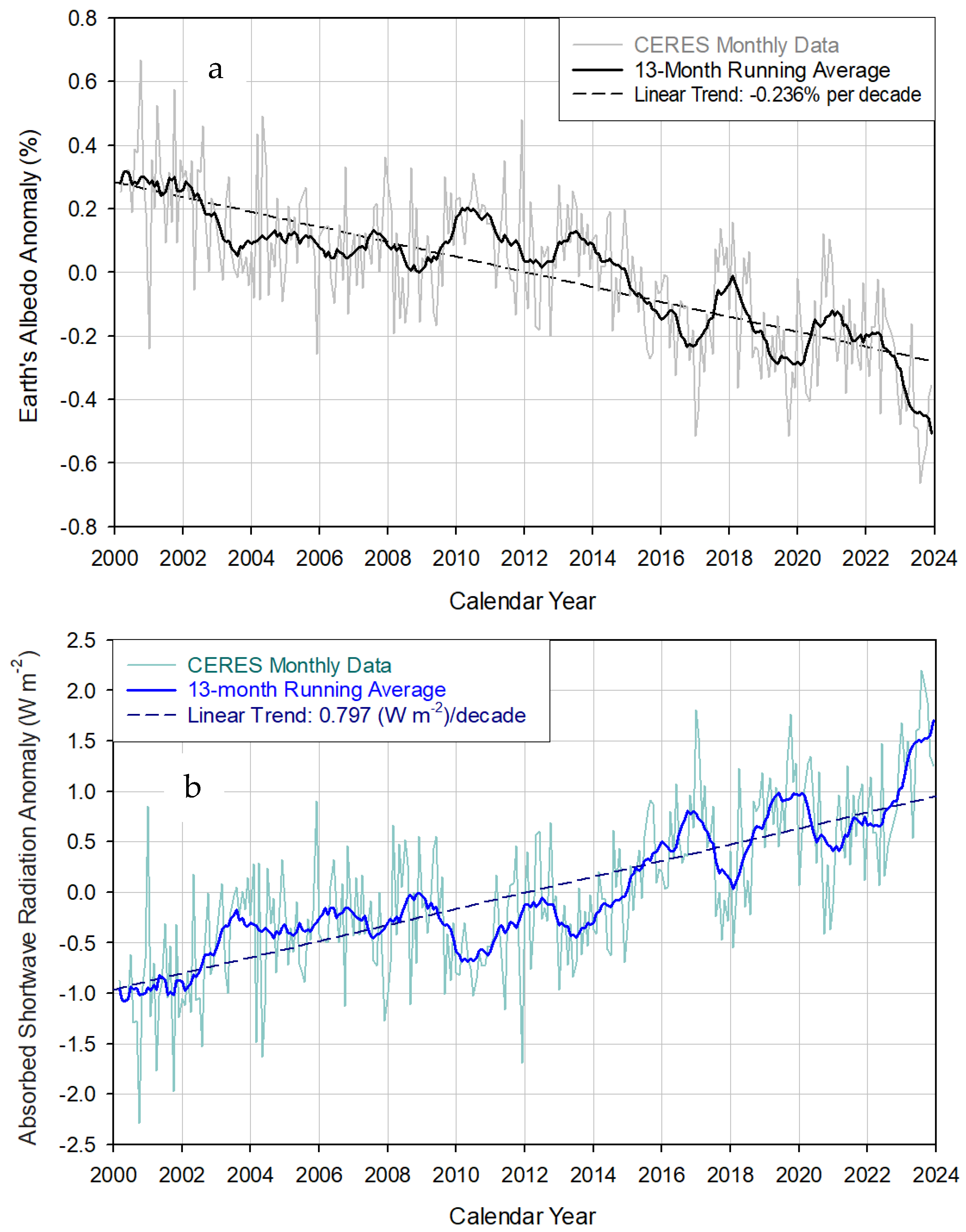
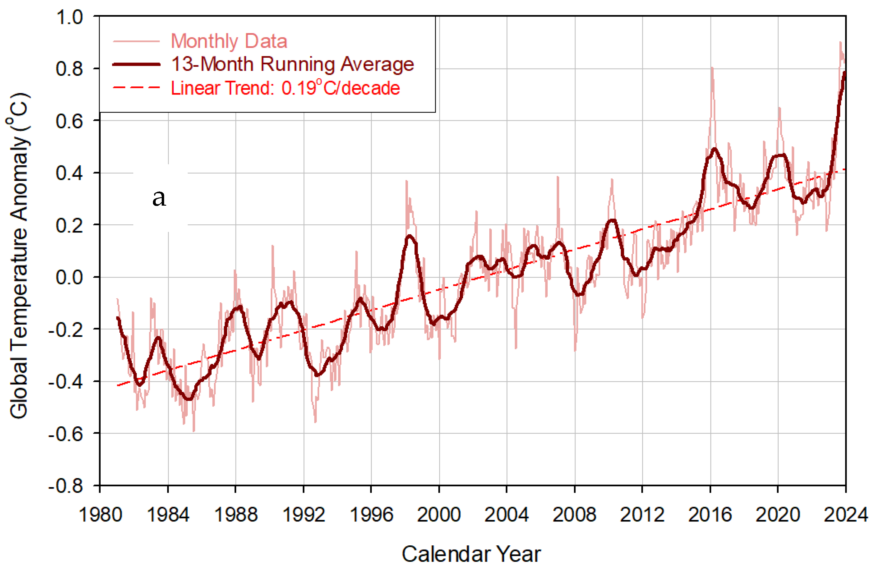
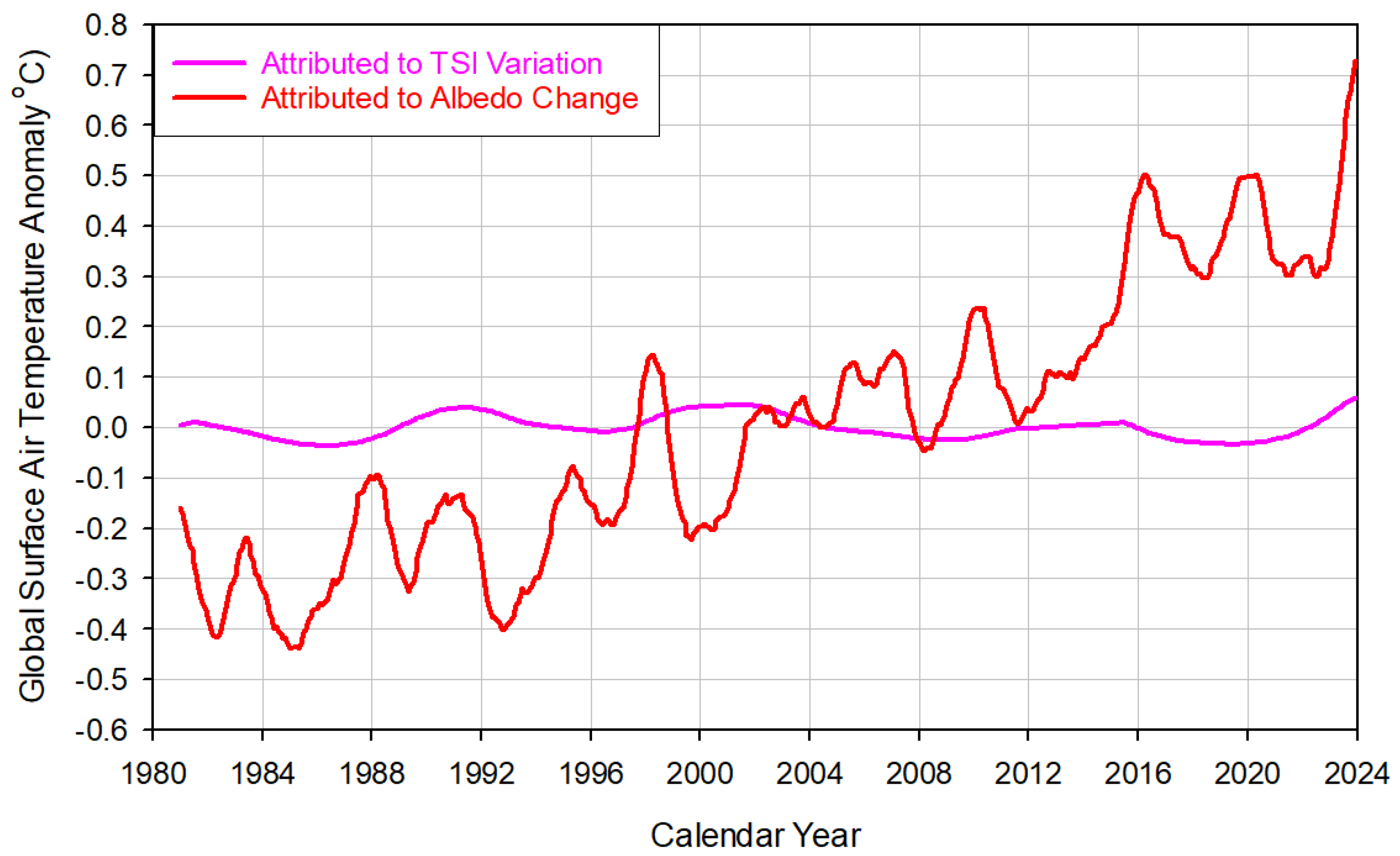
3.1. Drivers of Recent Warming

Figure 7 depicts the relationship between the observed anomalies of Earth’s absorbed shortwave radiation (from Figure 1b) and the planet’s GSAT (from Figure 5b) using 13-month running averages (note that the temperature series in Figure 5b has been re-referenced to its 2000–2023 mean in Figure 7). The GSAT anomalies track changes in the absorbed solar flux with a variable lag of 0 to 9 months (the average lag is approximately 4 months). This close empirical relationship suggests a direct control of the absorbed solar flux on GSAT. Dividing the measured surface warming trend (0.23 K/decade) by the observed trend of the absorbed solar flux (0.797 (W m⁻²)/decade) produces an empirical estimate of the Earth’s climate sensitivity to absorbed shortwave radiation: 0.288 K/(W m⁻²). For comparison, Equation (15b), which solely quantifies the effect of absorbed solar fluxes on GSAT, yields a climate sensitivity of 0.297 K/(W m⁻²). The close agreement between these two estimates, along with the slightly higher value of the modeled sensitivity, indicates that the observed warming during the past 24 years was likely caused by a planet-wide increase of shortwave-radiation absorption resulting from a decrease of Earth’s albedo.

Figure 8 portrays the relationship between Earth’s absorbed shortwave anomaly reported by CERES EBAF 4.2 and the mean temperature of the upper 100 m layer of the World’s Ocean, provided by the IAP 4.0 Subsurface Temperature dataset [11]. The IPCC AR6 attributes the ocean warming in recent decades to heat trapping by increasing concentrations of atmospheric greenhouse gases [2]. This implies that the oceans have been warmed by an increased flux of atmospheric downwelling longwave (LW) radiation. However, it is well-known that thermal radiation only penetrates less than a millimeter into sea water before it is completely absorbed and, therefore, cannot directly warm the deep ocean. Wong and Minnett [16] proposed a solution to this physical limitation by hypothesizing that the atmospheric LW radiation impedes the rate of heat transfer between deeper ocean and the atmosphere by reducing the vertical temperature gradient in a submillimeter-thick film of ocean water at the surface, called the Thermal Skin Layer (TSL). Thus, according to these authors, the atmospheric LW radiation heats the ocean indirectly by reducing the rate of deep-ocean cooling through the TSL. This idea is analogous to the proposed mechanism of the atmospheric “greenhouse effect” assumed to warm the planet’s surface by retaining (trapping) radiant heat that would otherwise escape into Space. However, Wong & Minnett did not explain how a TSL can form and remain intact in the open ocean, where the top 100–200 m layer is subjected to intense turbulent mixing by winds, which results in a uniform vertical temperature profile in that layer [17,18]. Also, these authors did not consider the observed decadal rise of surface shortwave radiation as a potential heating mechanism. Figure 8 shows that the mean annual temperature of the top 100 m ocean water closely follows changes in the absorbed solar flux by the planet. The dynamics of this flux explains 80% of the observed interannual ocean temperature variability in the upper mixed layer. Unlike the LW radiation, sunlight easily penetrates to a depth of 100 m and more in the ocean. Hence, the CERES data strongly suggest that, for the past 2.4 decades, the global ocean has been heated directly by shortwave radiation rather than indirectly by atmospheric thermal radiation thought to modify a hypothetical TSL and cause heat retention in the deeper ocean. Figure 8 also reveals that the climate sensitivity of the upper 100 m global ocean is 0.145/0.797 = 0.182 K/(W m⁻²), which is approximately 38% lower than the Earth’s overall climate sensitivity estimated from our model and the data series shown in Figure 7. The lower climate sensitivity of the upper ocean is explained by a higher heat capacity of sea water compared to the average heat capacity of Earth’s surface.

Figure 9a compares observed and modeled GSAT anomalies since March of 2000. The modeled time series is generated by Equation (16) using CERES-reported TOA anomalies of TSI and albedo as input (Figure 1a and Figure 2). The modeled temperature trend is 0.24 K/decade, while the observed trend is 0.23 K/decade. Both time series exhibit virtually identical El Niño-Southern Oscillation (ENSO) cycles, which suggests that ENSO events are externally driven by solar forcing via albedo variations rather than caused by internal factors such as the release of heat from the Equatorial Pacific Ocean as currently believed. Our model explained 100% of the Earth’s multidecadal warming trend and 83% of the GSAT interannual variability over the past 24 years. These results prompt the following question: If the observed solar forcing fully accounts for the global temperature rise since 2000, what is the role of the anthropogenic radiative forcing attributed to increasing greenhouse gases in recent warming?

The IPCC AR6 estimated that the Total Anthropogenic Forcing (TAF) from 1750 to 2019 (i.e., over 270 years) was 2.72 (1.96–3.48) W m⁻² [2]. Forster et al. [19] updated this estimate to 2.91 (2.19–3.63) W m⁻² for the period 1750–2022. The extra absorption of solar energy by Earth over the past 24 years alone was 2.7 W m⁻² (Figure 1b). Also, between 2011 and 2022, TAF rose 0.61 W m⁻² according to climate-model calculations discussed by Forster et al. [19], while the uptake of shortwave energy measured by CERES increased by 1.13 W m⁻², i.e., nearly twice as much as TAF. These facts suggest that the measured solar forcing is much stronger than the modeled TAF. If the 1.17 W m⁻² increase of TAF estimated by IPCC AR6 from 2000 to 2022 [14] was as effective at heating the planet as the observed 1.98 W m⁻² rise of Earth’s shortwave absorption (Figure 1b), then we should have seen an additional warming of at least 0.34 K over this 23-year period, assuming a climate sensitivity of 0.29 K/(W m⁻²). If we employ a climate sensitivity of 0.48 K/(W m⁻²) calculated from the GSAT record in Figure 5 and TAF data for 2011 and 2022 presented by Forster et al. [19] in their Table 3, then the additional warming should have been 0.56 K. This 21st-century transient climate sensitivity is almost identical to the long-term sensitivity of 0.47 K/(W m⁻²) calculated from the modeled TAF value of 2.72 W m⁻² and its 1.29 K contribution to the GSAT increase estimated by the IPCC AR6 from 1750 to 2019 [2] (Sections 7.3.5.2 and 7.3.5.3, respectively). Finally, if we use the IPCC’s Equilibrium Climate Sensitivity (ECS) of 0.76 K/(W m⁻²) calculated from the projected average global warming of 3.0 K by climate models in response to an effective radiative forcing of 3.93 W m⁻² due to a CO₂ doubling [2], then we should have witnessed an extra warming of 0.89 K over the period 2000–2023.

The fact that no warming has been observed above and beyond the amount expected from the measured solar forcing alone suggests a lack of physical reality to the theoretical greenhouse-gas radiative forcing. It also indicates the absence of positive feedbacks in the real climate system, such as the water-vapor, surface-albedo, and net cloud feedback hypothesized by IPCC AR6 to amplify the GSAT response [2] (Section 7.4). This is because Equation (16) contains no feedback mechanisms, yet it accurately describes both the observed GSAT evolution (including ENSO cycles) and the overall warming trend during the past 24 years. This evidence also suggests that the IPCC AR6 WG1 overestimated Earth’s climate sensitivity by 56% to 158%.

The above interpretation with respect to the missing effects of anthropogenic forcing and amplifying feedbacks are also supported by the inability of climate models to explain the 2023 unusual heat anomaly through greenhouse-gas variations and reductions of human aerosol emissions. Dr. Gavin Shmidt, Director of the NASA Goddard Institute for Space Studies, acknowledged this fact in a recent Nature World View article, where he stated: “In general, the 2023 temperature anomaly has come out of the blue, revealing an unprecedented knowledge gap perhaps for the first time since about 40 years ago, when satellite data began offering modellers an unparalleled, real-time view of Earth’s climate system” [20].

Interestingly, it is precisely the “real-time view” of satellite data with the above perspective in mind that provides a full explanation for the unusual heat anomaly in 2023. Figure 10a shows observed variations of the absorbed solar flux, TSI, and GSAT between Jan. 2019 and Dec. 2023. The 2023 rapid warming distinctly appears to have begun in February of 2021 in response to a solar forcing primarily caused by an increased shortwave absorption aided by a simultaneously rising TSI. Figure 10b compares observed and modeled GSAT anomalies. As in Figure 9a, the modeled ${\mathsf{\Delta }T}_t$ time series was produced by Equation (16) based solely on the solar forcings reported by CERES. It is clear from Figure 10 that a sudden decrease of Earth’s albedo, accompanied by a slight increase in TSI, caused a sharp increase in the uptake of solar energy by the climate system, which led to a spike of the global temperature in 2023. More importantly, however, Figure 1a and Figure 9 suggest that the 2023 heat anomaly was just another (albeit more extreme) manifestation of the same mechanism that has been lowering Earth’s albedo for the past 24 years and maintaining a warming trend of 0.23 K/decade. Hence, the “knowledge gap” argued by Schmidt [20] is not in the ability of current science to identify the immediate cause of the 2023 heat anomaly, which was a sharp drop in the albedo unrelated to human industrial emissions. The actual “gap” is in our understanding of (and ability to predict) the cosmic (and other unknown) forces controlling the Earth’s albedo via the process of cloud formation.

It is beyond the scope of this paper to analyze in depth the cause for the missing effects of model-generated greenhouse-gas radiative forcing and positive feedbacks on the observed warming for the past 2.4 decades. We will only point out that the above findings implicating solar forcing as the sole driver of recent warming is fully consistent with a recent discovery made by Nikolov and Zeller [12] about the adiabatic nature of the Atmospheric Thermal Effect (ATE), as illustrated in Figure 6. According to their findings, planetary atmospheres warm the surface of rocky celestial bodies not by trapping radiant heat (i.e., via impeding the surface infrared cooling to Space) as currently believed, but adiabatically through the force of total air pressure resulting from the action of gravity on atmospheric mass. This makes ATE independent of atmospheric composition, as demonstrated by vetted NASA planetary observations and the relationship in Figure 6. In this new paradigm of understanding, the atmospheric longwave radiation is merely a byproduct (i.e., an effect) of air temperatures rather than a driver of climate. From a standpoint of the Gas Law, the thermal kinetic energy of the atmosphere is determined by two factors: the absorbed solar flux (a diabatic process) and its thermodynamic enhancement by gas pressure (a quasi-adiabatic process). Therefore, the atmospheric longwave radiation is simply a manifestation of the ambient thermal energy already present in the climate system rather than an external source of heat as assumed by the greenhouse theory. Hence, the downwelling atmospheric LW flux does not contribute to the planet’s GSAT.

This implies that a global longwave radiative forcing predicted by climate models and attributed to rising concentrations of atmospheric trace gases does not exist in reality. According to this new physical framework, the global climate can only change if either the mean atmospheric surface pressure is significantly altered or the amount of sunlight absorbed by the planet is modified, mainly through modulation of the cloud albedo (assuming, of course, there is no change in the planet’s mean annual distance from the Sun). The albedo mechanism of climate change is robustly demonstrated by the CERES measurements.

3.2. Contributions of TSI and Albedo Variations to Recent Warming

Since Equations (8) and (15a) quantify the individual effects of TSI and albedo variations on GSAT, these formulas can be employed to evaluate the contribution of each solar forcing to the overall global warming of the past 24 years. Figure 11 compares the observed GSAT evolution between Mar. 2000 and Dec. 2023 to the global temperature anomalies produced by Equations (8) and (15a) using CERES shortwave-flux data as input. Albedo changes appear to have been the dominant driver of GSAT in terms of both the long-term warming trend and interannual variability, while TSI has only played a minor, modulating role in recent decades. This conclusion is also supported by Figure 12, which depicts the GSAT evolution attributable separately to changes in albedo and TSI since 1981. The assumption that Earth’s albedo has been decreasing for the past 37 years (and thus driving climate change) is based on the latest version of the ISCCP-FH radiative-profile flux product by the International Satellite Cloud Climatology Project (ISCCP), which shows a 6.5% reduction of the global cloud-cover fraction between 1986 and 2018 [21]. CERES data confirm this cloud-cover decline during the 21st Century.

The lack of a sizable TSI effect on GSAT in Figure 11 and Figure 12 is explained by the small interannual variability and nearly zero trend in TSI (Figure 2), coupled with a low GSAT sensitivity to the TSI forcing. According to our model, the Earth’s climate sensitivity is 0.297 K/(W m⁻²) to the absorbed solar flux (Equation (15b)), but only 0.053 K/(W m⁻²) to TSI (Equation (8)). The GSAT sensitivity to an albedo change is −1.02 K per 1% increase of albedo (Equation (15a)). Thus, the Earth’s climate is 5.6 times more sensitive to changes in sunlight absorption than to TSI variations. This estimate agrees well with empirical results reported by Shaviv [22] regarding the effect of TSI cycles on several climatic variables. This author found that “the total radiative forcing associated with solar cycles variations is about 5 to 7 times larger than just those associated with the TSI variations”. Shaviv did not propose a specific TSI amplification mechanism, but our analysis indicates that this is likely the cloud albedo-mediated change of Earth’s shortwave-radiation absorption.

These results indicate that TSI in and of itself is a rather weak driver of climate on decadal time scales. Therefore, climate research should focus on deciphering and quantifying the physical processes controlling the albedo dynamics of Earth and particularly that of clouds. The current available evidence points toward cosmic forcings such as galactic cosmic rays, solar interplanetary magnetic fields, and solar wind interreacting with the Earth’s global electric circuit as likely drivers of the cloud–albedo variations [23,24,25,26,27,28].

4. Discussion

Our analysis of the CERES EBAF 4.2 shortwave fluxes showed that the observed surface and subsurface ocean warming since 2000 (including the 2023 extreme heat anomaly) was exclusively caused by an increased uptake of solar energy due to a decreasing planetary albedo (Figure 7, Figure 8 and Figure 9). Thus, the available empirical evidence does not support the existence of an anthropogenic radiative forcing disturbing the energy flow within the Earth’s climate system. However, if the recent warming was not caused by heat-trapping greenhouse gases (as is often assumed), then what is the true physical nature of the Earth’s Energy Imbalance (EEI) observed by CERES and other monitoring platforms and widely reported in the scientific literature [29,30,31,32,33]?

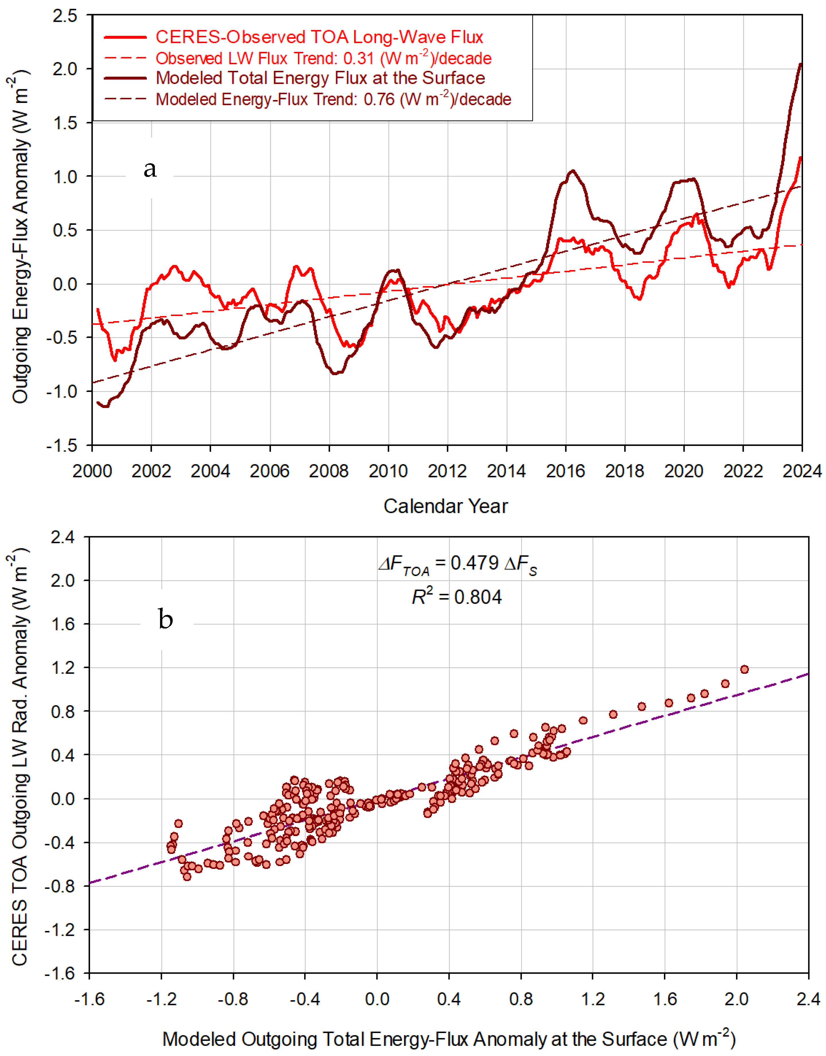
4.1. The Earth Energy Imbalance

Simply put, EEI is a difference between the absorbed solar flux and the outgoing LW infrared radiation at the TOA [8]. In the CERES dataset, EEI is called “Net Flux”. According to CERES observations, EEI has been increasing at a rate of 0.5 (W m⁻²)/decade from Mar. 2000 through Dec. 2023 due to the fact that Earth’s rising shortwave absorption has been outpacing the rate of the planet’s infrared cooling to Space. Loeb et al. [8] reported the same EEI trend for the period mid-2005–2019. The average EEI over the CERES monitoring period is 0.81 W m⁻², which is in good agreement with the IPCC AR6 estimate of 0.79 (0.52–1.06) W m⁻² for the period 2006–2018 [2] (Section 7.2.2.2), the 0.87 ± 0.12 W m⁻² estimate by von Schuckmann et al. [32] for the period 2010–2018, and the most recent estimate of 0.76 ± 0.2 W m⁻² by von Schuckmann et al. [33] for the period 2006–2020.

The international scientific community has unambiguously attributed EEI to an anthropogenic increase of atmospheric greenhouse gases such as CO₂ and methane based on the a priori assumption that these gases retain heat in the troposphere by impeding the Earth’s infrared cooling to Space [2,33]. Therefore, a positive EEI has been interpreted as evidence of heat accumulation in the climate system that commits Earth to future warming for decades and even centuries to come [32,33]. This belief has prompted climate scientists to start integrating the EEI estimates over space and time for different periods in order to come up with total heat/energy gain by the Earth system measured in Zetta Joules (1 ZJ = 10²¹ Joule). For example, the IPCC AR6 states that, due to heat trapping by greenhouse gases, the Earth had a net energy gain of 289.2 ZJ over the period 1993–2018 and 152.4 ZJ over the period 2006–2018 [2] (Section 7.2.2.2). As a result of such an interpretation, EEI is currently considered “the most fundamental indicator for climate change” and was proposed by an international team of 68 research collaborators to be implemented in the Paris Agreement’s Global Stocktake as a science-based measure of the World’s progress toward “bringing anthropogenic climate change under control” [33]. The fundamental assumption behind this proposal is that a reduction of the atmospheric CO₂ concentration to 353 ppm via the limiting of anthropogenic carbon emissions would eliminate the 0.87 W m⁻² EEI (estimated for the period 2010–2018) by increasing thermal radiation to Space, thus restoring Earth’s energy balance and stabilizing the climate [32]. Interestingly, however, only 1–2% of the Earth’s heat gain attributed to EEI is estimated to have accumulated in the atmosphere, causing the observed surface global warming for the last 50 years. The remaining 98–99% of the estimated energy gain is believed to have been stored under the surface (i.e., in the oceans, land masses, and glaciers) [2,33]. However, the published studies do not explain how 98% of the heat supposedly trapped in the troposphere by increasing greenhouse gases is transported below the Earth surface, when it is well-known that net fluxes of turbulent and radiative heat exchange flow upward and away from the surface on average.

A quick examination of the relationship between the CERES-measured EEI and GSAT over the past 24 years reveals that the global temperature is only poorly correlated with EEI (Figure 13). Unlike the solar forcing, which explains 83% of the GSAT interannual variability (see Figure 9), EEI only explains 36% of it (Figure 13b). This is because EEI is calculated as a difference between two time series that are out-of-phase with each other. The absorbed SW radiation generally precedes GSAT variations by approximately 4 months, while the outgoing LW radiation is completely in-phase with the GSAT anomalies.

As discussed in Section 3.1, the CERES data do not support the hypothesis that the observed EEI is a result of heat trapping by increasing atmospheric greenhouse gases. Instead, these data indicate that the Earth system has gained energy through an increased absorption of solar radiation (Figure 7, Figure 8 and Figure 9). The observed GSAT lag with respect to the absorbed shortwave flux implies that the solar energy is only retained (stored) in the system for a few months until it satisfies the volumetric heat capacity of the surface, and then radiates out through changes in the surface temperature. There is no sign of heat retention for more than a year in any component of the climate system. This evidence calls for a new explanation of the observed long-term EEI.

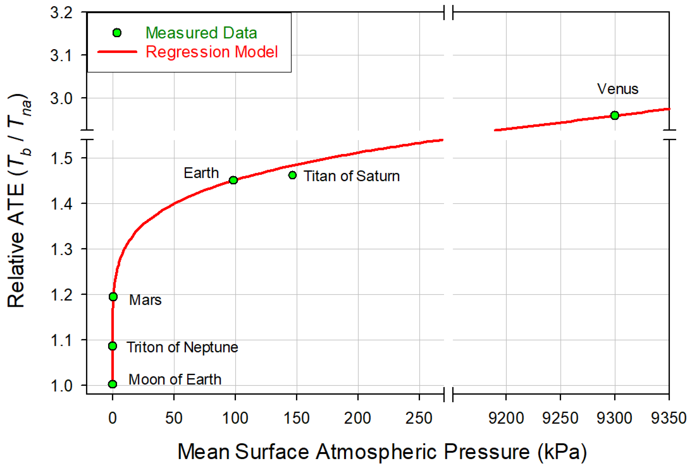
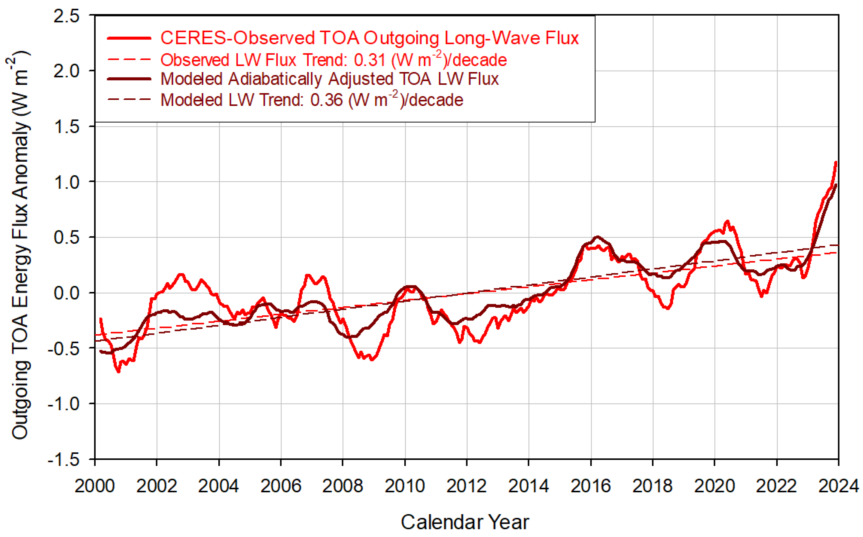
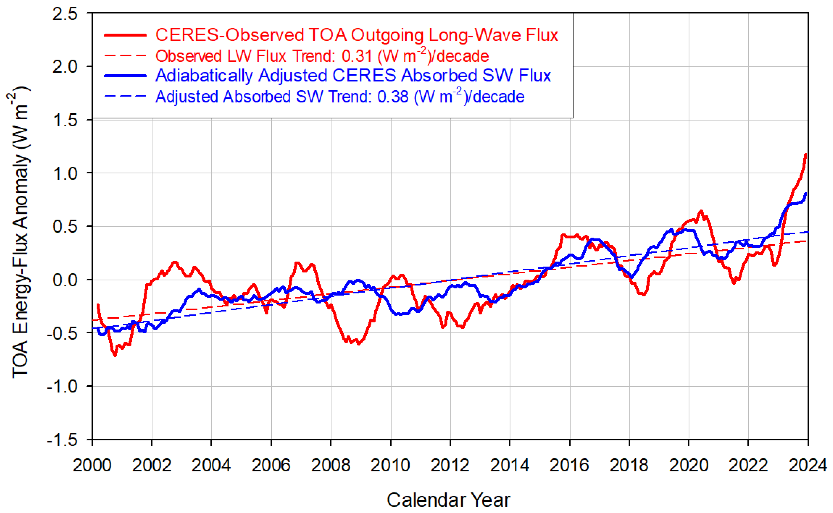
4.2. Physical Nature of the Earth Energy Imbalance

In order to decipher the physical nature of EEI, we first compared variations of the total surface energy flux resulting from GSAT responses to solar forcing with the LW flux anomalies measured by CERES at the TOA. Since the absorbed solar flux has been the driver of GSAT for the past 24 years (see the discussion in Section 3), Equation (15b) can be solved for the solar-flux anomaly term ($\mathsf{\Delta }{s}_a$) and the resulting expression combined with observed GSAT anomalies to estimate changes in the total energy flux at the surface. We denote the surface flux anomaly by $\mathsf{\Delta }{F}_S$ (W m⁻²) to semantically distinguish it from $\mathsf{\Delta }{s}_a$, although they are physically equivalent. From Equation (15b), we derive the following expression for $\mathsf{\Delta }{F}_S$:

$$\mathsf{\Delta }{F}_S={\displaystyle \frac{S}{4}}\left(1-{\alpha }_b\right)\left[{\left(1+{\displaystyle \frac{\mathsf{\Delta }T}{T_b}}\right)}^4-1\right]$$

(17)

where $\mathsf{\Delta }T$ is the observed GSAT anomaly depicted in Figure 5b as a 13-month running mean, and $S$ is the absolute TSI calculated by adding the baseline value $S_b=1360.85$ W m⁻² to the 13-month running average TSI anomaly depicted in Figure 2. Note that $\mathsf{\Delta }{F}_S$ and $\mathsf{\Delta }{s}_a$ are physically equivalent quantities, since the absorbed shortwave anomalies are fully converted into surface energy fluxes once GSAT responds to the solar forcing.

Figure 14 compares the outgoing TOA LW flux anomalies reported by CERES with the surface energy flux anomalies calculated by Equation (17). The two time-series are highly correlated (R² > 0.8) and exhibit clear positive trends over the 24-year period, as expected from a warming environment and the 2nd Law of Thermodynamics. However, the surface energy flux increases 2.45 times faster than the TOA LW flux (Figure 14a). This is because the magnitude of the measured TOA LW anomalies ($\mathsf{\Delta }{F}_{TOA}$, W m⁻²) is on average less than half the size of surface fluxes (Figure 14b). As shown in Figure 14b, the relationship between $\mathsf{\Delta }{F}_S$ and $\mathsf{\Delta }{F}_{TOA}$ is $\mathsf{\Delta }{F}_{TOA}=0.479 \mathsf{\Delta }{F}_S$. In other words, only 47.9% of the energy flux emitted by the surface reaches the TOA and is detected as an outgoing LW radiation to Space. This tropospheric flux attenuation is key to understanding the observed EEI.

We find an almost identical ratio of the upwelling energy fluxes between TOA and the surface in the all-sky global mean energy budget of Earth depicted in Figure 7.2 of the IPCC AR6 [2] (Section 7.2.1) and reproduced here as Figure 15 for convenience. The IPCC energy-budget diagram, which is said to represent climate conditions at the beginning of the 21st century, shows a total outgoing surface energy flux of 501 W m⁻², calculated as a sum of the upwelling LW radiation (398 W m⁻²), sensible heat flux (21 W m⁻²), and total evaporation or latent heat flux (82 W m⁻²). The TOA outgoing thermal flux is shown as 239 W m⁻². This yields a Tropospheric Energy-Flux Attenuation Coefficient (TEFAC) of 239/501 = 0.477. The CERES data suggest an average TOA thermal upwelling flux of 240.1 W m⁻² during the first 4 years of the 21st Century. Using this slightly higher measured value exactly reproduces the TEFAC derived from our model and shown in Figure 14b, i.e., 240.1/501 = 0.479. The fact that both the flux anomalies and the Earth’s steady-state global energy budget reveal the same TEFAC is not a coincidence, but it does indicate a common underlying physical mechanism.

The above evidence prompts the question, what causes the surface energy fluxes to dissipate (i.e., lose strength) while traversing the troposphere? The answer is provided by basic atmospheric physics outlined in textbooks and taught in college-level atmospheric-science classes. The altitude-dependent reduction of surface energy fluxes in the troposphere results from quasi-adiabatic cooling caused by a decreasing atmospheric pressure with height. An energy flux emitted at the surface is mostly intercepted by air masses adjacent to the surface. When an air parcel is heated, either radiatively or by conduction/convection, it rises and expands into lower pressure levels aloft. This makes the air parcel perform work on the surrounding atmosphere and lose a part of its thermal kinetic energy as a result, which reduces its internal temperature. By the time a convecting air parcel reaches a certain altitude, where it can radiate to Space unobstructed, its temperature is already significantly lower than that of the surface, which reduces the magnitude of the emitted LW radiative flux as well. Therefore, the observed energy-flux attenuation between surface and TOA is not a measure of atmospheric “heat trapping” as a priori assumed by the greenhouse climate theory [34,35], but instead represents a quasi-adiabatic loss of thermal energy in rising convective currents while crossing a field of decreasing air pressure.

The mechanism of vertical quasi-adiabatic cooling can also formally be described using fundamental thermodynamic relationships. Due to the importance of this novel interpretation of EEI, it would be beneficial to review these relationships here.

The Earth Energy Imbalance Explained by Thermodynamic Theory

The decrease of pressure with altitude is a consequence of a necessary atmospheric condition called hydrostatic equilibrium. The stable existence of a planetary atmosphere requires that, at every altitude, the outwardly directed force of pressure is balanced on average by the inwardly directed force of gravity. In mathematical terms, the hydrostatic equilibrium condition is described by the differential equation:

$${\displaystyle \frac{dP}{dz}}=-\rho g$$

(18a)

where $z$ is the altitude (m asl), $\rho$ is the air density (kg m⁻³) at altitude $z$, and $g$ is the gravitational acceleration (m s⁻²). According to the Ideal Gas Law, density is a function of pressure (P, Pa), temperature (T, K), atmospheric molar mass (M, kg/mol), and the universal gas constant (R = 8.314 J mol⁻¹ K⁻¹), i.e., ρ = PM/(RT). Also, the temperature at an altitude z can be described as a function of the surface temperature $T_o$ (K) and a lapse rate $L$ (K/m), i.e., ${T=T}_o+Lz$. Replacing the air density and temperature at altitude z in Equation (18a) with their equivalents followed by a separation of variables and integration of both sides over levels of pressure and altitude yields the following integral equation:

$${\int }_{P_o}^{P_z}{\displaystyle \frac{dP}{P}}=-{\displaystyle \frac{Mg}{R}} {\int }_0^Z{\displaystyle \frac{dz}{T_o+Lz}}$$

(18b)

The solution to Equation (18b) is the well-known barometric formula:

$$P_z=P_o{\left({\displaystyle \frac{T_o}{T_o+Lz}}\right)}^{{\displaystyle \frac{Mg}{RL}}}$$

(18c)

where $P_z$ is the air pressures at altitude $z$ and $P_o$ is the surface atmospheric pressure. Figure 16 illustrates the change of air pressure with altitude in the troposphere according to Equation (18c) for three different lapse rates: dry adiabatic (−9.8 K/km), humid environmental (−6.5 K/m), and moist adiabatic (−5.0 K/km). Note that, for any given set of $P_o$ and $T_o$ values, the vertical pressure profile exhibits a rather low sensitivity to changes in the lapse rate, $L$. Thus, the decrease of pressure with altitude is exclusively a consequence of the hydrostatic-equilibrium requirement (Equation (18a)).

The troposphere is thermodynamically governed by a polytropic process, where the expansion and compression of air accompanying vertical convection are not fully adiabatic but involve some transfer of energy between convecting air parcels and the surrounding environment. A polytropic process obeys the general relation [36]:

$$P{V}^n=C$$

(19)

where $P$ is the gas pressure (Pa), $V$ is the gas volume (m³), $n$ is the polytropic index, and $C$ is a constant. Equation (19) implies that the product $P{V}^n$ is invariant with altitude in the troposphere.

The polytropic index can assume a wide range of values in the general case of a thermodynamic system. However, in planetary atmospheres, we find $1.0<n<C_p/C_v$, where $C_p$ and $C_v$ are the specific heat capacities of air at constant pressure (_p) and at constant volume (v), respectively. The ratio ${\gamma =C}_p/C_v$ is known as the adiabatic index, since it is key in describing a standard adiabatic process. For the Earth’s atmosphere, $C_p$ = 1005 J kg⁻¹ K⁻¹ and $C_v$ = 718 J kg⁻¹ K⁻¹, which numerically restricts the polytropic index to the range $1.0<n<1.4$. This implies that the thermodynamic state of the troposphere lies somewhere between isothermal ($n=1.0$) and isentropic ($n=1.4$). The term “isentropic” means “constant entropy” and refers to an adiabatic process that is fully reversable. In an isentropic process, the thermal kinetic energy and temperature of an air parcel only change as a result of work done on or by the parcel (e.g., compression or expansion) without any heat exchange with the surrounding environment. In the real atmosphere, however, air parcels gain and lose heat due to water-vapor condensation and the vaporization of water droplets, respectively. Evaporation typically cools the near-surface environment, while condensation of water vapor at higher altitudes warms the upper troposphere through the release of latent heat, which reduces the absolute temperature lapse rate below its dry adiabatic value of 9.8 K/km. In addition, the atmosphere directly intercepts approximately a third of the total solar radiation absorbed by the planet while emitting LW radiation to Space. Nevertheless, the heat exchange between convective air parcels and the surrounding environment is not efficient enough to create an isothermal troposphere. As a result, the thermodynamics of the troposphere becomes quasi-adiabatic, where typically $1.1<n<1.4$. For the Earth’s standard atmosphere with an average tropospheric lapse rate of −6.5 K/km, the polytropic index is $n\approx 1.235$.

The process described by Equation (19) can also be presented in terms of pressure ($P$, Pa) and temperature ($T$, K). Since, according to the Gas Law, $V\propto T/P$, relation (19) can be written as:

$$P^{1-n}{T}^n=C$$

(20)

Equation (20) can be used to derive a general relationship between temperature and air pressure in the troposphere. A polytropic process implies the equality:

$${P_z}^{1-n}{{ T}_z}^n={P_o}^{1-n}{{ T}_o}^n$$

(21)

where the subscripts z and o refer to an altitude $z$ and the surface, respectively. Solving Equation (21) for the air temperature at an altitude $z$ produces:

$${ T}_z={ T}_o{\left({\displaystyle \frac{P_z}{P_o}}\right)}^{{\displaystyle \frac{n-1}{n}}}$$

(22)

Based on the likely values of the polytropic index in Earth’s atmosphere discussed above, the exponent term on the right side of Equation (22) is expected to be in the range $0.0<\left(n-1\right)/n<0.286$. This formula shows that, in planetary atmospheres, the air temperature directly depends on pressure, although the exact quantitative relationship between these variables varies depending on the value of the polytropic index. Equation (22) also reveals that the effect of pressure on temperature is always relative and never absolute. This is because $T_z$ numerically depends on the specific values of ${ T}_o$ and ${ P}_o$.

For $n=C_p/C_v$ = 1.4, Equation (22) converges to the potential-temperature formula also known as Poisson’s relation derivable from the First Law of Thermodynamics and the Ideal Gas Law [37]:

$$\theta ={ T}_z{\left({\displaystyle \frac{P_o}{P_z}}\right)}^{{\displaystyle \frac{R_a}{C_p}}}$$

where $\theta$ is the potential temperature in K ($\theta ={ T}_o$) and $R_a=R/M$ is the mass-specific gas constant of air (287 J kg⁻¹ K⁻¹). The exponent $R_a/C_p$ in Poisson’s formula can be derived from the power term $(n-1)/n$ in Equation (22) by replacing the polytropic index with the specific heat ratio $C_p/C_v$ and applying Mayer’s relation for ideal gases, $R_a=C_p-C_v$.

In the context of the Gas Law, the product $PV$ defines the thermal kinetic energy of a gas (measured in Joules) that gives the gas its temperature. Using the polytropic relation in Equation (19), it can be shown mathematically that the tropospheric thermal energy at an altitude $z$ ($P_z{V}_z$) relative to the thermal energy of air at the surface ($P_o{V}_o$) is given by the expression:

$${\displaystyle \frac{P_z{V}_z}{P_o{V}_o}}={\left({\displaystyle \frac{P_z}{P_o}}\right)}^{{\displaystyle \frac{n-1}{n}}}$$

(23)

Figure 17 illustrates the change of this relative thermal kinetic energy across vertical pressure levels and altitudes for three values of the polytropic index and the corresponding lapse rates describing dry, humid, and moist air, respectively. This graph illuminates a key fact that the thermal energy of the troposphere decreases with elevation due to an increasing depressurization of the environment. The energy fluxes emitted by the surface become attenuated (weakened) while travelling vertically through the troposphere precisely because of this environmental depressurization.

One can combine Equations (18c) and (22) to derive a formula (based on standard thermodynamics) that calculates the tropospheric energy-flux attenuation coefficient, ${\mathsf{\Phi }}_a$, as a ratio of the outgoing LW radiation flux at the TOA to the upwelling total energy flux at the surface. From Equation (22) and the Stefan–Boltzmann radiation law (relating an object’s absolute temperature to its radiant flux), it follows that:

$${\mathsf{\Phi }}_a={\displaystyle \frac{1}{f}}{\left({\displaystyle \frac{{ T}_z}{{ T}_o}}\right)}^4={\displaystyle \frac{1}{f}}{\left({\displaystyle \frac{P_z}{P_o}}\right)}^{4{\displaystyle \frac{n-1}{n}}}$$

(24)

where $f$ is a ratio of the total upwelling surface energy flux to the upwelling surface LW flux. This scaling parameter serves to adjust the surface infrared flux proportional to ${T_o}^4$ to match the observed total energy flux, which also includes non-radiative turbulent fluxes.

From the IPCC Earth’s energy-budget diagram in Figure 15, it follows that $f=501/398=1.259$, which implies $1/f=0.794$. Upon substituting $P_z$ into Equation (24) with its equivalent from Equation (18c), we obtain:

$${\mathsf{\Phi }}_a(z)=0.794{\left({\displaystyle \frac{T_o}{T_o+Lz}}\right)}^{4{\displaystyle \frac{Mg\left(n-1\right)}{RLn}}}$$

(25)

Using typical mean global values for the Earth’s current climate and atmosphere, i.e., $T_o$= 287.5 K, $M$ = 0.029 kg/mol, and $g$ = 9.8 ms⁻², the above thermodynamic equation can be applied to compute TEFAC by specifying an effective altitude $Z_e$, where the Earth’s thermal radiation escapes to Space. It is known that the Earth’s effective emission height is between 5000 and 5700 m asl, depending on the lapse rate [38,39]. Equation (25) reproduces the TEFAC value of 0.479 inferred from our model (see Figure 14b) at altitude $Z_e$ = 5250 m if $n=1.235$, corresponding to $L$ = −0.0065 K/m (−6.5 K/km). Between 5300 m and 5000 m altitude, Equation (25) yields $0.477{\le \mathsf{\Phi }}_a\le 0.491$, which covers the range of empirical TEFAC estimates. For $n=1.213$ corresponding to $L$ = −0.006 K/m (−6.0 K/km), Equation (25) predicts ${\mathsf{\Phi }}_a\left(Z_e\right)=0.478$ at altitude $Z_e$ = 5700 m. Hence, this thermodynamic formula explains the observed attenuation of thermal energy in the troposphere as a function of decreasing atmospheric pressure with height.

These results suggest that the standard definition of the atmospheric greenhouse effect as a difference of upwelling LW radiative fluxes between the surface and the TOA [34,35] is misleading at best, because such a difference does not quantify a tropospheric absorption (or retention) of outgoing radiant heat as assumed by climate theory. Instead, it describes an adiabatic dissipation (loss) of thermal energy in upward-moving convective currents. Furthermore, the above flux-based definition produces odd results when applied regionally, such as over central Antarctica, where it yields zero or negative greenhouse effect [40,41]. The actual Atmospheric Thermal Effect (ATE) over this region can be calculated as a difference between the mean annual surface temperatures of interior Antarctica (~230 K) and the Moon’s south pole (~90 K). Our Moon is a perfect airless equivalent of Earth, since it orbits the Sun at the same distance as our planet and has a very similar average surface albedo as Earth (~13%) [13]. Moon temperatures have been measured and gridded by the Diviner Lunar Radiometer Experiment [42]. This calculation yields ATE = 230 K – 90 K = 140 K over central Antarctica, which further demonstrates a lack of physical meaning in the flux-based definition of the greenhouse effect.

The above evidence indicates that the surface energy fluxes driven by GSAT variations must be adjusted for the adiabatic cooling effect of the troposphere before comparing them to CERES measurements of upwelling thermal radiation at the TOA. Figure 18 depicts the outgoing LW anomalies reported by CERES and the modeled fluxes from Figure 14a after the latter have adiabatically been corrected using TEFAC = 0.477 as a multiplier based on the IPCC global energy-budget diagram in Figure 15. This correction brings the two data series very close to each other in terms of interannual variability and linear trends. One also finds a similarly close match between the outgoing thermal fluxes and the absorbed shortwave anomalies reported by CERES (Figure 1b) once the solar fluxes are multiplied by the same adiabatic attenuation coefficient (0.477). Figure 19 shows these results.

4.3. Recapitulation of Findings about the Earth Energy Imbalance

The above discussion shows that a planetary energy imbalance arises when energy fluxes generated at the surface in response to a time-varying sunlight absorption are attenuated on their way to the TOA as a result of an altitude-dependent ambient depressurization. This means that EEI is a byproduct of a variable planetary shortwave absorption, and it would only vanish if the Earth’s albedo stops changing and the planet’s uptake of solar energy stabilizes. This is unlikely to occur, however, because cloud–albedo fluctuations are perpetual, and will continue to cause warming and cooling periods on multiyear time scales in the future. In this regard, it is important to realize that a positive EEI observed over several decades does not imply heat accumulation in the Earth system that would commit the World to a continuous warming for decades to come, as is currently feared [33]. This is because EEI is not caused by heat retention (i.e., impedance of cooling) due to increasing atmospheric greenhouse gases, and therefore does not carry excess energy that can be stored in the oceans and later released to cause more warming as some researchers claim [43]. In other words, EEI does not represent a “warming in the pipeline”, but is a consequence of an adiabatic loss of thermal energy in ascending (convecting) air parcels in the troposphere. Hence, an integration of EEI over space and time is physically meaningless.

The conclusion that EEI has been misinterpreted as a driver of climate change is also supported by a significant logical contradiction found in Chapter 7 of the WG1 Contribution to the IPCC AR6 [2]. Section 7.2.2.2 of that Chapter entitled “Changes in the Global Energy Inventory” states that, between 1971 and 2018, only 1.3% of the 434.9 ZJ total energy gain resulting from EEI was stored in the atmosphere, while 98.7% was absorbed by the subsurface (mostly the Global Ocean). At the same time, Section 7.3.5 titled “Synthesis of Global Mean Radiative Forcing, Past and Future” shows that virtually the entire estimated anthropogenic forcing responsible for EEI is required to just explain the surface atmospheric warming with no energy left over to account for subsurface heat storage. Hence, there is a major misalignment in the energy-budget calculations of the IPCC AR6 that needs an urgent resolution.

The results portrayed in Figure 18 and Figure 19 strongly suggest that, after accounting for the quasi-adiabatic tropospheric cooling and the time lags of outgoing energy fluxes with respect to the absorbed solar flux, there is no actual EEI between the absorbed shortwave and outgoing thermal radiation at the TOA on a multiyear time scale. In other words, the energy imbalances observed during various time periods have been misinterpreted by researchers, and the multi-decadal “heat gains” calculated from such apparent imbalances [2] (Section 7.2.2.2) [32,33] are fictitious, since they represent energy that is adiabatically lost to the climate system.

The Earth has undoubtedly gained a significant amount of heat over the past 45 years due to a sustained increase in solar-radiation uptake, which is a completely different mechanism from the proposed theoretical trapping of radiant energy by greenhouse gases. The observed rapid (within-months) response of GSAT to changes in the solar forcing evident in Figure 7, along with the phase match between GSAT anomalies and the outgoing thermal fluxes at the TOA, indicates a lack of long-term heat storage in the system that could commit the planet to a prolonged future warming. In other words, the Earth would start cooling within a year, once the current positive trend of shortwave-radiation absorption reverses.

5. Conclusions

Analogous to the famous “follow-the-money” approach often adopted by the social and political sciences to explain human behavior and social movements, this study can be described as a “follow-the-energy” journey to investigate the causes of recent climate warming.

The IPCC AR6 Working Group I (WG1) concluded that well-mixed greenhouse gases were “very likely the main driver of tropospheric warming since 1979” [1]. However, Chapter 7 of the IPCC AR6 WG1 Contribution did not take into proper consideration the observed increase of solar radiation absorption by Earth in recent decades known as “global brightening” [2] (Section 7.2.2.3). The Report did not analyze the decrease of Earth’s shortwave reflectance evident in the CERES EBAF dataset over the past 20 years and its impact on GSAT. Published studies agree that the observed decrease of planetary albedo and the associated increase of solar-energy uptake by the planet must have had a significant impact on the global temperature. However, there has been no attempts thus far to quantify the actual effect of this solar forcing on GSAT. We tried to bridge this knowledge gap by developing a novel, non-statistical process model from First Principles that explicitly relates changes in TSI and albedo to global temperature anomalies. The model (Equation (16)) was derived from independent NASA planetary observations and basic rules of calculus without using Earth-specific data, greenhouse-gas radiative forcing, or positive (amplifying) feedbacks. Our goal was to verify the above IPCC AR6 conclusion by assessing the direct effect of measured changes in TSI and Earth’s sunlight absorption on the 21st-century global surface warming as documented by 6 temperature datasets.

Our analysis revealed that the solar forcing (i.e., TSI and albedo changes) measured by CERES explain 100% of the observed global warming trend and 83% of the interannual GSAT variability over the past 24 years (Figure 9), including the extreme 2023 heat anomaly (Figure 10). Albedo changes were found to be by far the dominant GSAT driver, while TSI variations only played a minor, modulating role (Figure 11 and Figure 12). The sustained increase of sunlight absorption by the planet was also identified as the most likely driver of ocean warming in recent decades based on a high correlation (R² = 0.8) between the shortwave radiation uptake and the mean annual temperature anomaly of the 0–100 m global oceanic layer (Figure 8). These results suggest a lack of physical reality to both the anthropogenic radiative forcing attributed to rising greenhouse gases and the positive (amplifying) feedbacks hypothesized by the greenhouse theory and simulated by climate models. This is because any real forcing (or amplifying feedback) outside of the increased planetary uptake of solar radiation would have produced additional warming above and beyond the amount explained by changes in the planetary albedo and TSI. However, no such extra warming is observed in the available temperature records. Hence, the anthropogenic radiative forcing and associated positive feedbacks are likely model artifacts rather than real phenomena. The empirical data and model calculations analyzed in our study also indicate that the Earth’s climate sensitivity to radiative forcing is only 0.29–0.30 K/(W m⁻²). Therefore, the greenhouse theory overestimates this parameter by 56–158%.

The lack of evidence for heat trapping by greenhouse gases in the climate system during the 21st Century raises an important question about the physical nature of the Earth’s Energy Imbalance (EEI). The latter is defined as the difference between the absorbed shortwave and outgoing LW flux at the TOA. EEI has been observed and calculated by various monitoring platforms for several decades. This index became a research focus in climate science during the past 15 years, because it has been perceived as evidence of anthropogenic heat accumulation (energy retention) in the Earth system that would commit the World to a prolonged future warming, even after human carbon emissions have reached a net-zero level. As a result of such a view, EEI is now called the “most fundamental indicator for climate change” [33]. However, our analysis of observed data, model calculations, and standard thermodynamic theory showed that EEI has been misinterpreted by the science community, since it arises from adiabatic dissipation of thermal energy in ascending air parcels in the troposphere due to a decreasing atmospheric pressure with height (see discussion in Section 4). Hence, integrating EEI over space and time in an effort to calculate some total “energy gain” by the Earth system, as done by researchers in recent years, is physically misleading, because EEI includes energy that was adiabatically lost to the system during the convective cooling process. Our analyses also showed that this energy imbalance results from a varying sunlight absorption by the planet and would only disappear if the Earth’s albedo stops changing and the uptake of shortwave radiation stabilizes, which is unlikely to ever occur. The reduction of human greenhouse-gas emissions cannot and will not affect EEI. Nevertheless, the Earth has gained a considerable amount of thermal energy over the past 45 years due to a sustained increase of shortwave-radiation uptake, which is a completely different mechanism from the theorized trapping of radiant heat by greenhouse gases, since it does not involve a hidden energy storage.

These findings call for a fundamental reconsideration of the current paradigm of understanding about climate change and related socio-economic initiatives aimed at drastic reductions of industrial carbon emissions at all costs. An important aspect of this paradigm shift should be the prioritized allocation of funds to support large-scale interdisciplinary research into the physical mechanisms controlling the Earth’s albedo and cloud physics, for these are the real drivers of climate on multidecadal time scales.

References

1. IPCC. Climate Change 2021: The Physical Science Basis. Contribution of Working Group I to the Sixth Assessment Report of the Intergovernmental Panel on Climate Change; Masson-Delmotte, V., Zhai, P., Pirani, A., Connors, S.L., Péan, C., Berger, S., Caud, N., Chen, Y., Goldfarb, L., Gomis, M.I., et al., Eds.; Cambridge University Press: Cambridge, UK; New York, NY, USA, 2021; 2391p. [Google Scholar] [CrossRef]
2. Forster, P.; Storelvmo, T.; Armour, K.; Collins, W.; Dufresne, J.L.; Frame, D.; Lunt, D.; Mauritsen, T.; Palmer, M.; Watanabe, M.; et al. The Earth’s Energy Budget, Climate Feedbacks, and Climate Sensitivity. In Climate Change 2021: The Physical Science Basis. Contribution of Working Group I to the Sixth Assessment Report of the Intergovernmental Panel on Climate Change; Masson-Delmotte, V., Zhai, P., Pirani, A., Connors, S.L., Péan, C., Berger, S., Caud, N., Chen, Y., Goldfarb, L., Gomis, M.I., et al., Eds.; Cambridge University Press: Cambridge, UK; New York, NY, USA, 2021; pp. 923–1054. [Google Scholar] [CrossRef]
3. Stanhill, G.; Achiman, O.; Rosa, R.; Cohen, S. The cause of solar dimming and brightening at the Earth’s surface during the last half century: Evidence from measurements of sunshine duration. J. Geophys. Res. Atmos. 2014, 119, 10902–10911. [Google Scholar] [CrossRef]
4. Yuan, M.; Leirvik, T.; Wild, M. Global trends in downward surface solar radiation from spatial interpolated ground observations during 1961–2019. J. Clim. 2021, 34, 9501–9521. [Google Scholar] [CrossRef]
5. Loeb, N.G.; Thorsen, T.J.; Norris, J.R.; Wang, H.; Su, W. Changes in Earth’s energy budget during and after the “pause” in global warming: An observational perspective. Climate 2018, 6, 62. [Google Scholar] [CrossRef]
6. Loeb, N.G.; Wang, H.; Rose, F.G.; Kato, S.; Smith Jr, W.L. Decomposing shortwave top-of-atmosphere and surface radiative flux variations in terms of surface and atmospheric contributions. J. Clim. 2019, 32, 5003–5019. [Google Scholar] [CrossRef]
7. Loeb, N.G.; Wang, H.; Allan, R.P.; Andrews, T.; Armour, K.; Cole, J.N.S.; Dufresne, J.; Forster, P.; Gettelman, A.; Guo, H.; et al. New generation of climate models track recent unprecedented changes in Earth’s radiation budget observed by CERES. Geophys. Res. Lett. 2020, 47, e2019GL086705. [Google Scholar] [CrossRef]
8. Loeb, N.G.; Johnson, G.C.; Thorsen, T.J.; Lyman, J.M.; Rose, F.G.; Kato, S. Satellite and ocean data reveal marked increase in Earth’s heating rate. Geophys. Res. Lett. 2021, 48, e2021GL093047. [Google Scholar] [CrossRef]
9. Dübal, H.-F.; Vahrenholt, F. Radiative energy flux variation from 2001–2020. Atmosphere 2021, 12, 1297. [Google Scholar] [CrossRef]
10. Stephens, G.L.; Hakuba, M.Z.; Kato, S.; Gettelman, A.; Dufresne, J.-L.; Andrews, T.; Cole, J.N.S.; Willen, U.; Mauritsen, T. The changing nature of Earth’s reflected sunlight. Proc. Roy. Soc. A 2022, 478, 20220053. [Google Scholar] [CrossRef]
11. Cheng, L.; Trenberth, K.E.; Fasullo, J.; Boyer, T.; Abraham, J.; Zhu, J. Improved estimates of ocean heat content from 1960 to 2015. Sci. Adv. 2017, 3, e1601545. [Google Scholar] [CrossRef]
12. Nikolov, N.; Zeller, K. New insights on the physical nature of the atmospheric Greenhouse Effect deduced from an empirical planetary temperature model. Environ. Pollut. Clim. Change 2017, 1, 112. [Google Scholar] [CrossRef]
13. Volokin, D.; ReLlez, L. On the average temperature of airless spherical bodies and the magnitude of Earth’s atmospheric thermal effect. SpringerPlus 2014, 3, 723. [Google Scholar] [CrossRef]
14. Scafetta, N. Empirical assessment of the role of the Sun in climate change using balanced multi-proxy solar records. Geosci. Front. 2023, 14, 101650. [Google Scholar] [CrossRef]
15. Jones, P.D.; Harpham, C. Estimation of the absolute surface air temperature of the Earth. J. Geophys. Res. Atmos. 2013, 118, 3213–3217. [Google Scholar] [CrossRef]
16. Wong, E.W.; Minnett, P.J. The response of the ocean thermal skin layer to variations in incident infrared radiation. J. Geophys. Res. Ocean. 2018, 123, 2475–2493. [Google Scholar] [CrossRef]
17. Akbari, E.; Alavipanah, S.K.; Jeihouni, M.; Hajeb, M.; Haase, D.; Alavipanah, S. A review of ocean/sea subsurface water temperature studies from remote sensing and non-remote sensing methods. Water 2017, 9, 936. [Google Scholar] [CrossRef]
18. Treguier, A.M.; Montégut, C.d.B.; Bozec, A.; Chassignet, E.P.; Fox-Kemper, B.; Hogg, A.M.; Iovino, D.; Kiss, A.E.; Le Sommer, J.; Li, Y.; et al. The mixed layer depth in the Ocean Model Intercomparison Project (OMIP): Impact of resolving mesoscale eddies. Geosci. Model Dev. 2023, 16, 3849–3872. [Google Scholar] [CrossRef]
19. Forster, P.M.; Smith, C.J.; Walsh, T.; Lamb, W.F.; Lamboll, R.; Hauser, M.; Ribes, A.; Rosen, D.; Gillett, N.; Palmer, M.D.; et al. Indicators of Global Climate Change 2022: Annual update of large-scale indicators of the state of the climate system and human influence. Earth Syst. Sci. Data 2023, 15, 2295–2327. [Google Scholar] [CrossRef]
20. Schmidt, G. Climate models can’t explain 2023’s huge heat anomaly—We could be in uncharted territory. Nature 2024, 627, 467. [Google Scholar] [CrossRef]
21. Zhang, Y.; Rossow, W.B. Global radiative flux profile data set: Revised and extended. J. Geophys. Res. Atmos. 2023, 128, e2022JD037340. [Google Scholar] [CrossRef]
22. Shaviv, N.J. Using the oceans as a calorimeter to quantify the solar radiative forcing. J. Geophys. Res. 2008, 113, A11101. [Google Scholar] [CrossRef]
23. Voiculescu, M.; Usoskin, I.; Condurache-Bota, S. Clouds blown by the solar wind. Environ. Res. Lett. 2013, 8, 045032. [Google Scholar] [CrossRef]
24. Lam, M.M.; Chisham, G.; Freeman, M.P. Solar wind-driven geopotential height anomalies originate in the Antarctic lower troposphere. Geophys. Res. Lett. 2014, 41, 6509–6514. [Google Scholar] [CrossRef]
25. Svensmark, J.; Enghoff, M.B.; Shaviv, N.; Svensmark, H. The response of clouds and aerosols to cosmic ray decreases. J. Geophys. Res. Space Physics. 2016, 121, 8152–8181. [Google Scholar] [CrossRef]
26. Svensmark, H.; Svensmark, J.; Enghoff, M.B.; Shaviv, N.J. Atmospheric ionization and cloud radiative forcing. Sci. Rep. 2021, 11, 19668. [Google Scholar] [CrossRef]
27. Kumar, V.; Dhaka, S.K.; Hitchman, M.H.; Yoden, S. The influence of solar-modulated regional circulations and galactic cosmic rays on global cloud distribution. Sci. Rep. 2023, 13, 3707. [Google Scholar] [CrossRef]
28. Miyahara, H.; Kusano, K.; Kataoka, R.; Shima, S.; Touber, E. Response of high-altitude clouds to the galactic cosmic ray cycles in tropical regions. Front. Earth Sci. 2023, 11, 1157753. [Google Scholar] [CrossRef]
29. Trenberth, K.E.; Fasullo, J.T.; Balmaseda, M.A. Earth’s Energy Imbalance. J. Clim. 2014, 27, 3129–3144. [Google Scholar] [CrossRef]
30. Trenberth, K.E.; Fasullo, J.T.; von Schuckmann, K.; Cheng, L. Insights into Earth’s energy imbalance from multiple sources. J. Clim. 2016, 29, 7495–7505. [Google Scholar] [CrossRef]
31. Raghuraman, S.P.; Paynter, D.; Ramaswamy, V. Anthropogenic forcing and response yield observed positive trend in Earth’s energy imbalance. Nat. Commun. 2021, 12, 4577. [Google Scholar] [CrossRef] [PubMed]
32. von Schuckmann, K.; Cheng, L.; Palmer, M.D.; Hansen, J.; Tassone, C.; Aich, V.; Adusumilli, S.; Beltrami, H.; Boyer, T.; Cuesta-Valero, F.J.; et al. Heat stored in the Earth system: Where does the energy go? Earth Syst. Sci. Data 2020, 12, 2013–2041. [Google Scholar] [CrossRef]
33. von Schuckmann, K.; Minière, A.; Gues, F.; Cuesta-Valero, F.J.; Kirchengast, G.; Adusumilli, S.; Straneo, F.; Ablain, M.; Allan, R.P.; Barker, P.M.; et al. Heat stored in the Earth system 1960–2020: Where does the energy go? Earth Syst. Sci. Data 2023, 15, 1675–1709. [Google Scholar] [CrossRef]
34. Raval, A.; Ramanathan, V. Observational determination of the greenhouse effect. Nature 1989, 342, 758–761. [Google Scholar] [CrossRef]
35. Schmidt, G.A.; Ruedy, R.A.; Miller, R.L.; Lacis, A.A. Attribution of the present-day total greenhouse effect. J. Geophys. Res. 2010, 115, D20106. [Google Scholar] [CrossRef]
36. Knight, R. All about polytropic processes. Phys. Teach. 2022, 60, 422. [Google Scholar] [CrossRef]
37. Andrews, D.G. An Introduction to Atmospheric Physics, 2nd ed.; Cambridge University Press: Cambridge, UK, 2010; pp. 24–26. [Google Scholar]
38. Pierrehumbert, R.T. Principles of Planetary Climate; Cambridge University Press: Cambridge, UK, 2010; 652p. [Google Scholar]
39. Dufresne, J.-L.; Eymet, V.; Crevoisier, C.; Grandpeix, J.-Y. Greenhouse effect: The relative contributions of emission height and total absorption. J. Clim. 2020, 33, 3827–3844. [Google Scholar] [CrossRef]
40. Schmithüsen, H.; Notholt, J.; König-Langlo, G.; Lemke, P.; Jung, T. How increasing CO2 leads to an increased negative greenhouse effect in Antarctica. Geophys. Res. Lett. 2015, 42, 10422–10428. [Google Scholar] [CrossRef]
41. Sejas, S.A.; Taylor, P.C.; Cai, M. Unmasking the negative greenhouse effect over the Antarctic Plateau. npj Clim Atmos Sci. 2018, 1, 17. [Google Scholar] [CrossRef] [PubMed]
42. Williams, J.-P.; Paige, D.A.; Greenhagen, B.T.; Sefton-Nash, E. The global surface temperatures of the Moon as measured by the Diviner Lunar Radiometer Experiment. Icarus 2017, 283, 300–325. [Google Scholar] [CrossRef]
43. Hansen, J.E.; Sato, M.; Simons, L.; Nazarenko, L.S.; Sangha, I.; Kharecha, P.; Zachos, J.C.; von Schuckmann, K.; Loeb, N.G.; Osman, M.B.; et al. Global warming in the pipeline. Oxf. Open Clim. Change 2023, 3, kgad008. [Google Scholar] [CrossRef]
Figure 1. Monthly radiative anomalies derived from the CERES EBAF 4.2 dataset: (a) Earth’s global albedo calculated via dividing the reflected all-sky shortwave anomaly by the globally averaged incident solar flux at the TOA (i.e., the global insolation) and multiplying the resulting fraction by 100 to convert to a percent; (b) Earth’s absorbed solar flux calculated via multiplying the CERES reflected all-sky shortwave anomaly by −1 based on the fact that radiation absorption is opposite (and complimentary) to reflection.
Geomatics 04 00017 g001
Figure 2. Deseasonalized monthly anomalies of the Total Solar Irradiance (TSI) calculated from CERES observations via multiplying the reported TOA global shortwave isolation anomalies by 4.0.
Geomatics 04 00017 g002
Figure 3. GSAT 13-month running mean anomalies from 7 datasets. Each time series is referenced to its respective mean over the period March 2000–December 2023. The satellite-based datasets report temperature changes in the lower troposphere (TLT) measured by Microwave Sounding Units (MSU), while surface-based databases are derived from thermometer readings on the ground.
Geomatics 04 00017 g003
Figure 4. Linear trends of 7 global surface and lower-troposphere temperature datasets over the period March 2000–December 2023. UAH was excluded from our analysis, because it showed an anomalously low rate of warming during the 21st Century (i.e., less than 0.18 °C/decade) compared to the other datasets.
Geomatics 04 00017 g004
Figure 5. GSAT monthly anomalies calculated by averaging of 6 global datasets (i.e., HadCRUT5, GISTEMP4, NOAA GlobalTemp, BEST, RSS, and NOAA STAR) and a 13-month running mean used to smooth the seasonal variability: (a) Over the period 1981–2023; (b) Over the CERES observational period (March 2000–December 2023).
Geomatics 04 00017 g005aGeomatics 04 00017 g005b
Figure 6. The Relative Atmospheric Thermal Effect/Enhancement (RATE) as a function of the mean surface atmospheric pressure across 6 well-studied planetary bodies with rocky surfaces in the Solar System. RATE is the ratio of a planet’s observed long-term GSAT under an atmosphere ( T b ) to the planet’s estimated global surface temperature without an atmosphere ( T n a ). The red curve is the result of non-linear regression analysis of NASA planetary data. See Nikolov & Zeller [12] for details.
Geomatics 04 00017 g006
Figure 7. Comparison between observed GSAT anomalies and CERES-reported changes in the Earth’s absorbed solar flux. The two data series, representing 13-month running means, are highly correlated with the absorbed SW flux, explaining 78% of the GSAT variation (R2 = 0.78). Also, GSAT lags the absorbed shortwave radiation between 0 and 9 months, which indicates that GSAT is controlled by changes in sunlight absorption.
Geomatics 04 00017 g007
Figure 8. Comparison between observed temperature anomalies of the upper 100 m global-ocean layer [11] and changes in the Earth’s absorbed solar flux reported by CERES. Both time series represent 13-month running averages. Although completely independent of each other, the data series are highly correlated with the absorbed SW flux, explaining 80% of the interannual ocean temperature variability (R2 = 0.80). Ocean temperatures are from the IAP 4.0 dataset (see Table 1) and were provided by Prof. Lijing Cheng at the Institute of Atmospheric Physics (IAP) of the Chinese Academy of Sciences.
Geomatics 04 00017 g008
Figure 9. Comparison of modeled and observed GSAT anomalies over the CERES monitoring period. The modeled curve is generated by Equation (16) using CERES-reported anomalies of albedo (Figure 1a) and TSI (Figure 2) as input. The observed GSAT lags the modeled temperature between 0 and 9 months, because GSAT lags the absorbed solar flux: (a) Time series of observed and modeled GSAT anomalies. The modeled temperature series has been shifted 4 months forward after June of 2007 to partially compensate for the lag in the observed GSAT series; (b) Scatter plot of observed vs. modeled GSAT anomalies. The dashed blue line is a linear regression. The solar forcing explains 100% of the multidecadal warming trend and 83% of the GSAT interannual variability after partially accounting for the lag of the observed GSAT, or 79% of the GSAT variability without accounting for lags (R2 = Correlation Coefficient; S = slope of the linear relationship).
Geomatics 04 00017 g009
Figure 10. Illustrating the cause of the 2023 global heat anomaly: (a) Observed GSAT in relation to changes of TSI and the absorbed shortwave radiation measured by CERES; (b) Observed GSAT in relation to the modeled global temperature response to solar forcing (TSI and albedo combined) according to Equation (16). The observed GSAT lags the modeled GSAT because global temperature lags changes in the absorbed solar flux.
Geomatics 04 00017 g010
Figure 11. Global surface temperature changes predicted in response to observed variations of TOA TSI (Equation (8)) and the planetary albedo (Equation (15a)) over the CERES monitoring period. These are compared to measured GSAT anomalies. The observed multi-decadal warming trend and the El Niño-Southern Oscillation (ENSO) cycles are almost entirely explained by changes in the Earth’s albedo, while TSI only has a small, almost inconsequential contribution.
Geomatics 04 00017 g011
Figure 12. Estimated contributions of TSI and albedo variations to the evolution of Earth’s GSAT since 1981. The TSI-induced temperature change is calculated by Equation (8) using ACRIM measurements of TSI [14]. The albedo-induced GSAT anomalies are estimated by subtracting the TSI contribution from the GSAT record shown in Figure 5a. The assumption that the cloud albedo has been decreasing since the mid-1980s is based on an observed reduction of the global cloud-cover fraction reported by the ISCCP-FH dataset [21].
Geomatics 04 00017 g012
Figure 13. Relationship between Earth’s Energy Imbalance (EEI) measured by CERES and GSAT anomalies based on 6 global datasets: (a) Comparison of GSAT and EEI time series representing 13-month running means; (b) Linear correlation between EEI and GSAT. The dashed red line is a linear regression. EEI only explains 36% of the GSAT interannual variability, while the solar forcing explains 83% of it (Figure 9).
Geomatics 04 00017 g013
Figure 14. Observed outgoing LW flux at the TOA by CERES and modeled total energy flux at the surface by Equation (17) using the GSAT record in Figure 5b as input: (a) Time series and trends of the observed and modeled fluxes; (b) Relationship between the modeled surface total energy-flux anomalies and the observed TOA upwelling thermal-flux anomalies. The dashed magenta line is a linear regression. The magnitude of the TOA flux anomalies is, on average, 47.9% the size of surface fluxes.
Geomatics 04 00017 g014
Figure 15. The global mean energy budget of Earth according to IPCC AR6 [2] (Section 7.2.1), their Figure 7.2. Numbers indicate the best estimates for magnitudes of the globally averaged energy balance components in W m−2, together with their uncertainty ranges in parentheses (5–95% confidence range), representing all-sky climate conditions at the beginning of the 21st century. According to this diagram, the Tropospheric Energy-Flux Attenuation Coefficient (TEFAC) is 239/(398 + 82 + 21) = 0.477.
Geomatics 04 00017 g015
Figure 16. Atmospheric pressure as a function of altitude according to the barometric formula (Equation (18c)) for three different lapse rates: dry adiabatic (L = −0.0098 K/m), humid environmental (L = −0.0065 K/m), and moist adiabatic (L = −0.005 K/m). Note that variations of the lapse rate only have a minor impact on the decrease of pressure with altitude.
Geomatics 04 00017 g016
Figure 17. Decrease of the thermal kinetic energy in the troposphere relative to the thermal kinetic energy of air at the surface for a standard atmosphere under 3 scenarios defined by different polytropic indices and temperature lapse rates applicable to dry, humid, or moist environments, respectively. According to the Gas Law, the thermal kinetic energy of air is defined by the product PV.
Geomatics 04 00017 g017
Figure 18. Comparison of observed and modeled outgoing thermal radiative fluxes at the TOA. The observed anomalies are from the CERES EBAF 4.2 dataset. The modeled time series is produced by multiplying the surface total-energy fluxes calculated by Equation (17) and shown in Figure 14a by 0.477 to account for the quasi-adiabatic energy dissipation in the troposphere. This correction makes the modeled timeseries agree almost perfectly with the observed timeseries.
Geomatics 04 00017 g018
Figure 19. CERES TOA outgoing LW fluxes compared to adiabatically adjusted CERES anomalies of the absorbed solar flux. The adiabatic adjustment consists of multiplying the original shortwave (SW) data series in Figure 1b by TEFAC = 0.477, inferred from the IPCC energy-budget diagram in Figure 15. This makes the absorbed solar flux closely match the trend and interannual variability of the outgoing LW radiation flux, which indicates that the Earth’s Energy Imbalance (EEI), quantified as a difference between absorbed shortwave and outgoing LW radiation at the TOA, is an artifact of a quasi-adiabatic tropospheric cooling driven by a decreasing pressure with altitude.
Geomatics 04 00017 g019