Review

Advances in Remote Sensing and Deep Learning in Coastal Boundary Extraction for Erosion Monitoring

by
Marc-André Blais
and
Moulay A. Akhloufi
*
Perception, Robotics and Intelligent Machines (PRIME), Department of Computer Science, Université de Moncton, Moncton, NB E1A 3E9, Canada
*
Author to whom correspondence should be addressed.
Geomatics 2025, 5(1), 9; https://doi.org/10.3390/geomatics5010009
Submission received: 12 December 2024 / Revised: 30 January 2025 / Accepted: 3 February 2025 / Published: 6 February 2025

Abstract

:
Erosion is a critical geological process that degrades soil and poses significant risks to human settlements and natural habitats. As climate change intensifies, effective coastal erosion management and prevention have become essential for our society and the health of our planet. Given the vast extent of coastal areas, erosion management efforts must prioritize the most vulnerable and critical regions. Identifying and prioritizing these areas is a complex task that requires the accurate monitoring and forecasting of erosion and its potential impacts. Various tools and techniques have been proposed to assess the risks, impacts and rates of coastal erosion. Specialized methods, such as the Coastal Vulnerability Index, have been specifically designed to evaluate the susceptibility of coastal areas to erosion. Coastal boundaries, a critical factor in coastal erosion monitoring, are typically extracted from remote sensing images. Due to the extensive scale of coastal areas and the complexity of the data, manually extracting coastal boundaries is challenging. Recently, artificial intelligence, particularly deep learning, has emerged as a promising and essential tool for this task. This review provides an in-depth analysis of remote sensing and deep learning for extracting coastal boundaries to assist in erosion monitoring. Various remote sensing imaging modalities (optical, thermal, radar), platforms (satellites, drones) and datasets are first presented to provide the context for this field. Artificial intelligence and its associated metrics are then discussed, followed by an exploration of deep learning algorithms for extracting coastal boundaries. The presented algorithms range from basic convolutional networks to encoder–decoder architectures and attention mechanisms. An overview of how these extracted boundaries and other deep learning algorithms can be utilized for monitoring coastal erosion is also provided. Finally, the current gaps, limitations and potential future directions in this field are identified. This review aims to offer critical insights into the future of erosion monitoring and management through deep learning-based boundary extraction.

1. Introduction

Erosion, a powerful geological process, involves the gradual wearing away of surface material by natural forces such as water and wind. These forces break down hardened materials through mechanisms such as abrasion, hydraulic action and chemical weathering. As particles are broken down into smaller and lighter forms, and they are transported to new locations. While erosion has shaped landscapes and enabled the formation of complex ecosystems, it also has significant drawbacks. As soil erodes, agricultural land is lost [1], nutrients are depleted [2] and coastal areas are destroyed [3]. Coastal erosion, which refers to the gradual retreat of coastlines, shorelines and beaches, poses risks to both humans and the biosphere. Coastal areas are vital to human populations due to their economic, ecological and social importance. Notably, 40% of the global population lives within 100 km of the coast [4], while 53% and 38% of USA imports and exports are sea-based [5], underscoring the importance of coastal regions. Additionally, humans rely on these areas for resources such as food and raw materials, including sand, lime, minerals and oil. Wildlife, flora and microorganisms also depend heavily on coastal areas for feeding, mating and survival.
Natural techniques and barriers have evolved over time to manage and mitigate coastal erosion. Dense vegetation [6], sand dunes [7], coral reefs [8] and rocky shorelines [9] play key roles in protecting coastal zones. However, these natural defenses are increasingly threatened by human activities such as urban development [10,11,12], the mismanagement of ecosystems [13] and climate change [14,15]. Climate change worsens coastal erosion through rising sea levels and increased storm frequency [16]. As coastal areas erode, human infrastructures such as homes, roads and ports face destruction, while complex ecosystems are forced to adapt or vanish. Conservation efforts such as replanting vegetation [17] and constructing artificial sand dunes [7,18] or coral reefs [19] can help protect these areas. Monitoring, assessing and forecasting coastal erosion are crucial for managing and directing these efforts. On-site surveys provide highly accurate data, using methods like Global Positioning System (GPS) tracking. However, these techniques are limited by the vast size and inaccessibility of many coastal areas. Remote sensing is often employed to gather data on coastal regions using high-altitude platforms such as aircraft, drones and satellites. These platforms are equipped with sensors like multispectral cameras and radars to capture various information.
Remote sensing images, combined with historical numerical data, are highly valuable for coastal erosion monitoring and assessment [20,21,22]. The Coastal Vulnerability Index (CVI), a widely utilized assessment tool, measures the vulnerability of coastal areas across different scales. It has been applied to assess coastal vulnerability to erosion [23,24], flooding [25] and rising sea levels [26]. Remote sensing data, indices, tidal information and marine surveys can be integrated into multidisciplinary approaches for effective erosion monitoring [27]. However, many of these assessment tools rely on historical coastal boundary data, such as coastlines and shorelines, making their extraction essential. Some reviews have highlighted the reliance on manual inspection for extracting boundaries from remote sensing images [28,29]. However, manual extraction is time-consuming, as it requires experts to analyze and track coastal boundaries across multiple years and data sources. Artificial Intelligence (AI), particularly Machine Learning (ML), has been proposed as a tool to assist in this task. ML can automatically extract coastal boundaries and track changes over time, significantly reducing the time required for the expert evaluation of remote sensing data. Several works demonstrated the application of traditional ML algorithms combined with remote sensing data for shoreline monitoring [30]. However, traditional ML approaches often rely on hand-crafted features, additional numerical data, and extensive fine-tuning, and they are typically region-specific, which limits their usability. Deep Learning (DL), a subset of ML, has emerged as a promising alternative, leveraging Neural Networks (NNs) to learn directly from data instead of relying on predefined rules. DL offers unique advantages in remote sensing and coastal boundary extraction. Convolutional Neural Networks (CNNs), for example, can process high-resolution remote sensing images to generate segmentation maps and extract coastal boundaries. CNNs and other DL algorithms can process hundreds of images per minute with minimal human intervention or preprocessing. This capability enables DL algorithms to be seamlessly integrated into live monitoring systems aboard airplanes and drones. Using live data for coastal analysis provides researchers with instant access to information, which is particularly valuable during natural events such as storms and surges. Small-scale operations using planes and drones are especially appealing due to their cost-effectiveness compared to more expensive alternatives [31,32]. Satellites, on the other hand, offer consistent and predictable global coverage, providing extensive historical data and accessibility.
This review aims to provide a comprehensive overview of how DL can be applied to extract coastal boundaries from remote sensing images for erosion monitoring. The focus on DL is driven by its success in related tasks, such as image segmentation and contour extraction. In Section 2, we first introduce the methodology used for the collection and selection of the various articles presented. Foundational knowledge on remote sensing, satellite-based acquisition platforms, datasets, AI and the associated evaluation metrics is then presented in Section 3 and Section 4. We then review studies employing DL and remote sensing data for coastal boundary extraction, covering segmentation, direct extraction techniques and a combination of both in Section 5, Section 6 and Section 7.
This review emphasizes coastal boundary extraction, specifically focusing on coastlines and shorelines, as tracking these features is essential for monitoring coastal changes. The shoreline is defined as a dynamic boundary where the sea meets the land, influenced by daily tides and seasonal variations. In contrast, the coastline represents a more static boundary, typically on a larger scale, such as the edge of a continent. Sea-land segmentation refers to the separation of sea and land in remote sensing images without specifying a particular boundary. Most studies do not differentiate between these terms, likely due to the similarities in the underlying algorithms used, regardless of spatial scale. As such, this review treats these terms as a unified concept. Section 8 explores how these extracted boundaries and DL can be leveraged in tools for assessing and monitoring erosion, while Section 9 presents a discussion on the reviewed data and studies. Finally, we discuss current limitations, challenges and future directions in this field in Section 10, integrating these insights throughout the review. Figure 1 provides a visual representation of the review structure and its key components.

2. Methodology

The primary objective of this study is to provide a literature review on the use of DL for coastal boundary extraction in erosion monitoring. First, we searched for existing reviews on this topic to establish the current state of the art, using keywords such as review, deep learning, coastline and remote sensing. Building on insights from these reviews, we refined our search by selecting additional keywords to identify related studies. Combinations of coastal boundary, coastline, coast, shore, shoreline, sea–land segmentation, coastal segmentation, extraction, detection, deep learning, remote sensing and satellite were systematically searched across IEEE Xplore, Google Scholar, Google and Elicit AI. References cited in relevant articles were analyzed to identify additional sources, while the Google Scholar cited by tool was used to discover further related works. We only included studies that directly applied DL to coastal boundary extraction or segmentation, excluding those focused on inland water bodies. To ensure a comprehensive review, no date restrictions were imposed, though all articles were published before December 2024.
To generate the thematic structure shown in Figure 1, we manually categorized articles based on their primary focus and methodological approach. This manual approach accounted for subtle nuances and methodological variations that automated clustering techniques might overlook. Specifically, we identified recurring themes in reviewed papers and assigned them to the most appropriate category, such as coastal boundary extraction, segmentation and dual approaches. This process ensured that we not only presented the relevant work in the field but also provided the appropriate context for the selected studies. As this review aims to support erosion monitoring, we also conducted a focused search on risk assessment, vulnerability and erosion evaluation tools. Keywords such as risk assessment, coastal erosion, coast erosion prediction, coastal vulnerability index and coastal monitoring were used to identify relevant studies for Section 8. This additional search ensured that our review encompassed DL applications in risk evaluation, further enhancing its relevance to coastal erosion monitoring. The resulting structure includes two context sections (Remote Sensing and AI), two boundary extraction sections (Segmentation and Direct Extraction), an Erosion Assessment section and a Future Directions section.

3. Remote Sensing

Remote sensing involves capturing information about the Earth’s surface from high altitudes. Sensors mounted on satellites, aircraft, or Unmanned Aerial Vehicles (UAVs) collect data in various modalities, utilizing either passive or active sensors. This section presents an overview of passive and active sensors, the satellite-based platforms available for remote sensing and publicly available boundary databases and specialized datasets. Understanding the availability of such data enables researchers to develop realistic and scalable solutions.

3.1. Passive Sensors

Passive sensors capture sunlight reflected across various ranges within the electromagnetic spectrum (ES). Figure 2 illustrates a portion of the ES and the types of data associated with each region.
Visible bands span from 400 to 700 nanometers (nm), while infrared (IR) bands extend from 700 to 100,000 nm [33,34]. The wavelength of spectral bands determines the type of information captured by sensors. The visible and IR ranges can identify vegetation loss [35], soil degradation [36] and moisture levels [37]. Panchromatic (PAN) images use a single wide band to capture the entire visible spectrum. Although PAN images offer high spatial resolution, they have low spectral resolution, producing monochromatic images.
Narrow visible bands, such as blue, green and red, provide specific information compared to the PAN band, as follows:
  • Blue band: Used for monitoring water quality, turbidity and shallow water characteristics.
  • Green band: Differentiates vegetation from water and aids in land use mapping.
  • Red band: Assesses vegetation health, crop conditions and soil properties.
IR bands, including Near-Infrared (NIR), Short-Wave Infrared (SWIR), Mid-Wave Infrared (MWIR) and Long-Wave Infrared (LWIR), provide a broad range of spectral information, as follows:
  • NIR: Monitors vegetation health, detects water bodies and supports land use mapping.
  • SWIR: Measures soil moisture, identifies fires and differentiates materials such as minerals and rocks.
  • MWIR: Tracks land and sea surface temperatures, monitors thermal variations and detects fires.
  • LWIR: Analyzes surface temperature, soil composition, urban activity and heat stress.
For coastal erosion monitoring, NIR and SWIR bands are particularly valuable. Table 1 summarizes key spectral bands and their applications. Using single bands enables the targeted evaluation of specific features such as vegetation health or soil moisture while reducing data complexity, which can improve efficiency and result interpretability. However, individual bands are limited in spectral information and are more susceptible to atmospheric distortions, such as haze, clouds and rain.
Multispectral data combines individual bands to enhance the perceived spectral information. The true color composite (Red-Green-Blue), mimicking human vision, is widely used in remote sensing to extract water bodies [38] or assess land usage [39]. Red-Green-Blue (RGB) images use three narrow bands, providing higher spectral resolution but often lower spatial resolution compared to PAN images. Pan-sharpening, which fuses PAN and multispectral images, offers a middle-ground solution. Figure 3 demonstrates the differences between PAN, RGB and pan-sharpened images of the same region, showcasing the increase in resolution.
False-color composites, such as NIR-Red-Green (FC1) and NIR-SWIR1-Red (FC2), offer alternatives to RGB composites. Vegetation appears brighter in FC1, which is valuable for analyzing vegetation density and protection against coastal erosion [40]. FC2 is sensitive to moisture, enabling the more accurate differentiation of waterways in suboptimal conditions [41]. Figure 4 compares FC1, FC2 and RGB images of the same region, highlighting their differences. While FC2 images excel in delineating waterways, their resolution is often lower than FC1 and RGB images due to the coarser resolution of the SWIR band.
Indices based on multiple individual bands can extract specific information highly relevant to coastal erosion [42]. For example, the Normalized Difference Vegetation Index (NDVI) and Normalized Difference Water Index (NDWI) use NIR combined with red or green bands to monitor vegetation health and biomass density [43] or differentiate water bodies from land [44]. These indices are defined as follows:
NDVI = NIR Red NIR + Red
NDWI = Green NIR Green + NIR
The Modified NDWI (MNDWI), shown in Equation (3), replaces the NIR band in NDWI with SWIR to enhance water body detection in complex scenarios [45].
MNDWI = Green SWIR Green + SWIR
Additionally, the Moisture Index provides an overview of soil and vegetation moisture content and is defined as follows:
Moisture Index = NIR SWIR NIR + SWIR
Figure 5 visualizes the NDVI, NDWI, MNDWI and Moisture Index for the same region, highlighting their diverse applications in erosion monitoring.
Overall, multispectral composites and indices provide valuable information about terrain, vegetation and moisture, which are critical for erosion monitoring. Passive sensors, while energy-efficient due to their reliance on reflected sunlight, are limited by weather and lighting conditions, making them less effective for continuous and live monitoring tasks.

3.2. Active Sensors

Active sensors, an alternative to passive sensors, emit their own signals, such as microwaves or lasers, to capture reflected signals from the Earth. These signals can penetrate fog, clouds and rain, enabling consistent data acquisition regardless of lighting and weather conditions. The Synthetic Aperture Radar (SAR), a widely used active sensor, emits microwave signals to measure backscatter, providing crucial information on soil, terrain and ground texture. SAR data are invaluable for erosion management due to the SAR’s ability to monitor soil moisture [46], vegetation structure [47], surface changes [48] and ocean features [49].
Polarization is a parameter in SAR instruments that consists of the orientation of the transmitted and received signal waves. Depending on the orientation of the two signals, either horizontal (H) or vertical (V) for each signal, different information is captured.
  • Single-polarization: Usually sends and receives signals in one orientation (HH or VV) but can also generate HV and VH signals.
  • Dual-polarization: Transmits in one orientation and receives in two (HH and HV or VH and VV), providing higher-quality data which can be used to distinguish different types of surfaces.
  • Full-polarization: Transmits and receives signals in both orientations, producing all four combinations (HH, HV, VH, VV) simultaneously.
HH is useful in detecting human infrastructure, bodies of water and smooth surfaces, while VV, HV and VH are better suited to capture vegetation and surface roughness. SAR instruments also vary by wavelength:
  • X-band: Short wavelength for detecting small changes and urban monitoring.
  • C-band: Suitable for global mapping and identifying crops, with moderate canopy penetration.
  • L-band: Long wavelength for biomass monitoring, with better canopy and soil penetration but lower resolution.
Light Detection and Ranging (LiDAR) uses laser pulses to generate precise 3D maps of the terrain, natural features and human-made structures. Different LiDAR products include Digital Elevation Models (DEMs), Digital Surface Models (DSMs) and Digital Terrain Models (DTMs). Topographic LiDAR, using NIR lasers, maps land surfaces [50], while Bathymetric LiDAR, using green lasers, can monitor underwater terrain [51].
Active sensors offer several advantages over passive sensors, particularly their ability to penetrate fog, clouds, haze and snow. These properties allow them to collect consistent data regardless of weather, time or lighting conditions, making them highly interesting for coastal erosion monitoring. Their capacity to capture reliable and predictable data ensures accurate and consistent measurements over time. Additionally, active sensors can generate detailed topographical information, which is valuable for understanding terrain features such as elevation and land formation. These data are crucial for modeling processes like erosion and flooding, providing insights into how terrain changes over time and under varying environmental conditions. However, the benefits of active sensors come with notable challenges. Unlike passive sensors, active sensors must generate their own signals, which requires significantly more energy. This energy demand reduces their ability to capture continuous data, limiting the duration and coverage of their monitoring capabilities. Active sensors are also more expensive and often provide lower resolution compared to passive sensors, which can make them less practical for large-scale monitoring efforts. These factors can hinder their widespread application in projects requiring extensive geographic coverage or prolonged observation periods. Nonetheless, active sensors offer unique and highly valuable data that complement other monitoring techniques. Their ability to capture data under challenging environmental conditions and to provide critical topographical insights makes them a valuable tool for coastal monitoring, especially in regions with adverse weather or complex terrain.

3.3. Remote Sensing Platforms

Satellites, aircraft and UAVs can be equipped with these sensors to collect highly valuable information about the Earth. Satellites provide extensive coverage and consistent data due to their predictable orbital paths, although access to high-resolution public data is often limited. Aircraft offer cost-effective alternatives but are constrained by limited coverage and frequency, typically providing mission-specific data. UAVs, ranging from lightweight drones to larger systems, offer flexibility in data acquisition but are generally restricted to smaller areas and specific missions. Airplanes and UAVs provide unique opportunities in the field of coastal erosion monitoring. Their relatively low cost and versatility make them ideal for deployment missions in coastal area monitoring [52,53]. The integration of UAVs into swarms would enable them to efficiently cover vast areas autonomously [54]. Incorporating DL solutions into large-scale swarms could facilitate the consistent and live monitoring of coastal areas. While drones and UAVs are well-suited for local deployment and real-time monitoring missions, they are not the primary focus of this review. This review emphasizes training DL algorithms for coastal boundary extraction, which requires large-scale datasets that are rarely accessible using these platforms.
Remote sensing satellites are ideal for acquiring data to train these models due to their large coverage and consistent orbital paths. Key factors when evaluating data acquisition platforms include sensor type, spectral bands and resolution, as a high resolution is essential for capturing small changes. Revisit time is crucial and refers to the duration required for a satellite or constellation of satellites to capture the same location. A shorter revisit time allows for more frequent data acquisition, enabling the collection of optimal and up-to-date information for the same location. Data availability and acquisition range are critical considerations for satellite-based remote sensing platforms. While commercial satellites provide higher-resolution data, their high costs often make them impractical for training large-scale DL models. Furthermore, the acquisition range of available data is essential for developing accurate forecasting models, which often rely on decades of historical records. Table 2 and Table 3 summarize the characteristics of passive and active satellites, respectively, including sensor types, resolutions, revisit times and data availability. Commercial constellations, such as WorldView, Pleiades and PlanetScope, provide high-resolution data with a daily revisit time, making them highly valuable for coastal boundary monitoring. On the other hand, public satellites such as Landsat and Sentinel provide coarser resolutions with a lower revisit time. However, public satellites offer their data freely and have archives of much older data available, making them ideal for academic research. Deployment missions would benefit from commercial satellites, while model development would benefit from public satellites due to their data accessibility.

3.4. Datasets

Since most DL algorithms require annotations to train their models, we first present coastal boundary databases that are free and publicly available. These databases can be combined with data gathered from satellites to generate coastal boundary datasets. We then discuss publicly available datasets that can be used for coastal boundary extraction and sea–land segmentation that require matching pairs of images and annotations.
The Global Coastline Explorer, provided by the United States Geological Survey (USGS) [55,56], contains more than four million coastline segments, each 1 km or shorter. Derived from 2014 Landsat satellite imagery, the dataset provides global shoreline vectors at a resolution of 30 m. Regions span five continents, 21,818 large islands and 318,868 small islands. The shoreline vectors are classified using the coastal and marine ecosystem classification standard. It includes 81,000 coastal segment units categorized into 16 ecological classes based on attributes such as slope, chlorophyll content and erodibility. The data are accessible via ArcGIS Online (Esri, Redlands, CA, USA) and can be paired with remote sensing imagery to generate labeled image–mask pairs.
The Global Self-consistent, Hierarchical, High-resolution Geography Database (GSHHG) is a collaboration between the University of Hawai’i and the National Oceanic and Atmospheric Administration (NOAA) [57]. It integrates the following three data sources: the World Vector Shorelines (global shorelines, excluding Antarctica), the CIA World Data Bank II (lakes, rivers, political borders) and the Atlas of the Cryosphere (Antarctic coastlines). The dataset includes five resolution levels, ranging from full (200 m) to crude (100 km) and six shoreline types from before 1996. Ten river classes are also provided, ranging from major rivers to irrigation canals. Available in ESRI shapefile and binary formats, the dataset is suitable for long-term research but less effective for short-term erosion studies due to its lower resolution.
Natural Earth Data [58] is a public dataset offering various cartographic and visualization resources. It includes cultural data (boundaries, roads), physical data (coastlines, rivers, glaciers) and raster data (shaded relief and ocean features). Physical data are available in shapefile format with resolutions of 10 m, 30 m and 100 m. OpenStreetMap (OSM) [59] provides a community-maintained global dataset, including coastlines represented as polygons that separate land from sea. Available in varying resolutions with WGS84 and Mercator projections, OSM data are widely accessible and can be used with remote sensing imagery.
Specialized datasets to train AI models for coastal boundary extraction and segmentation are limited. Despite the abundance of remote sensing data, only a few datasets for these tasks are publicly available. We present the key datasets identified for these applications, which offer both images and annotations. Seale et al. [60] proposed the Sentinel-2 Water Edges Dataset (SWED) [61]. SWED consists of 12 bands in the visible-IR range collected using Sentinel-2 from 2017 to 2021. Cloud-free images were selected by filtering the data based on the cloudy pixel percentage metadata. The selected scenes covered various regions of the world at both high and low tides, ensuring variety in the dataset. The bands, originally with resolutions ranging from 10 m to 60 m, were interpolated (nearest neighbor) to a resolution of 10 m per pixel. Corresponding masks were generated through semi-supervised clustering with QGIS (QGIS Development Team, Open Source Geospatial Foundation, Beaverton, OR, USA) and labeled land as 0 and sea as 1. The dataset includes 16 training pairs and 98 validation pairs of high-resolution image–mask pairs.
Yang et al. [62] proposed a matching segmentation image–mask dataset based on satellite images, named Sea-Land Segmentation (SLS). The data, captured from the Chinese region, was collected using Landsat-8 OLI at a resolution of 30 m. Chinese coastlines are particularly interesting as a quarter consists of muddy areas, a challenging scenario for coastline extraction. Images were collected from 2013 to 2018, with a maximum cloud coverage of 5%. Two composites, RGB and FC2, underwent radiometric calibration and atmospheric correction to normalize the images. Seventeen images were used for training and 12 for testing, which were further divided into 512 × 512 patches, resulting in 1950 training images and 1411 test images. The patches were manually segmented into land and sea using LabelMe software (MIT Computer Science and Artificial Intelligence Laboratory, Cambridge, MA, USA) [63].
Similarly, YTU-WaterNet [64] used 63 Landsat-8 OLI images to create a coastline dataset. The images were collected from various regions (Albania, Argentina, Bulgaria, England, Georgia, Greece, Ireland, Italy, Libya, Russia, South Africa, Spain, Turkey and the USA) to ensure geographic variety. The data were collected in different years (approximately 2017–2019), seasons and tide levels. The authors selected the Blue-Red-NIR bands for their effectiveness in distinguishing water from land. Segmentation maps were generated using OSM and the data were cropped into 512 × 512 sections, producing 824 training, 92 validation and 92 test images.
Scarpetta et al. [65] introduced a dataset for coastline extraction based on multispectral data. The images were collected using Sentinel-2 and consist of 13 bands processed to Level-1C, with resolutions ranging from 10 m to 60 m. The coastlines were derived from the Continually Updated Shoreline Product (CUSP), provided by NOAA. The data were carefully selected to ensure high accuracy, using only images captured after December 2016. Images from Alaska were excluded due to ice, while river areas were removed due to the low resolution. Regions spanned Hawai’i, Northwest and Northeast Continental USA, the Great Lakes, the Gulf of Mexico and Puerto Rico. A total of 155 tiles were selected and divided into patches (64 × 64) containing coastlines, which were labeled using automatic methods. Ultimately, the dataset contained 894 labeled tiles, each with 13 bands at a resolution of 10 m per pixel.
In continuation of Scarpetta et al. [65] Andria et al. [66] presented a new dataset, SNOWED, which can be used to train DL models for shoreline detection. Like their previous work, the shoreline data were sourced from NOAA CUSP, while Sentinel-2 satellite images provided multispectral data. The dataset includes images from coastal regions of the USA and the surrounding territories, covering an area up to 20 km inland and spanning June 2015 to 2023. Sentinel-2 images were selected with a cloud coverage below 10% and a maximum temporal offset of 30 days from the NOAA measurements. The NOAA shorelines were projected onto Sentinel-2 images and the Sentinel-2 scene classification was used to verify the masks. The dataset consists of 4334 labeled image–mask pairs, including all 13 Sentinel-2 bands. A visual inspection identified that approximately 17% of images had minor inconsistencies. To validate SNOWED, the authors trained a standard U-Net for sea–land segmentation and achieved good results.
The Coast-Train dataset [67] offers image–mask segmentation pairs containing aerial orthophotos and satellite images. The images were collected in the Pacific, Gulf of Mexico, Atlantic and Great Lakes regions of the USA between 2008 and 2021. The masks have a range of 1 to 12 classes out of 33 classes, including water, whitewater, bedrock, ice, vegetation and no data. Resolutions range from 0.05 m to 1 m for orthophotos and 10 m to 15 m for satellite images. The dataset was processed and augmented to create 502 training images and 34 validation images, all 512 × 512 pixels.
Pollard et al. [68] proposed a reference dataset for the analysis of shoreline and beach changes in the United-Kingdom (UK). The dataset combines vertical aerial photography, LiDAR and coastal surveys. Resolutions range from 0.1 m to 0.25 m for aerial photography, 0.25 m to 2 m for LiDAR and 200 m to 1000 m for surveys. The capture dates, respectively, ranged from 2001 to 2019, 1999–2009 and 2000–2019. The authors used various techniques to handle seasonal and tidal changes. For example, the vegetation line was used as a shoreline proxy due to its resistance against tidal changes. The dataset includes grayscale, RGB and RGB + IR bands. In addition, the authors provide methods for quantifying changes in sediment volume using LiDAR, enabling quantitative erosion monitoring. The dataset is publicly available and includes metadata for error quantification. This dataset is particularly interesting due to the high resolution and on-site measurement of the data.
Figure 6 shows the respective image–mask pairs of SWED [60], SLS [62] and YTU-WaterNet [64]. These examples demonstrate the data complexity found in coastal areas. Figure 6b shows a highly complex scenario with multiple islands. These scenarios are particularly challenging due to the numerous discontinuous boundaries located in close proximity to each other.
Table 4 provides an overview of the coastline datasets presented. Although some coastal boundary databases are available, the majority have a coarse resolution. This limitation makes them less valuable for erosion monitoring due to the lack of fine details. As shown in this table, specialized coastal boundary datasets are also limited, with only a few are publicly available. Most of these datasets also have a coarse resolution, often exceeding 10 m per pixel, making them less suitable for detailed erosion monitoring. However, two datasets [67,68] provide sub-meter resolution with matching annotations, making them ideal for boundary extraction.

4. Artificial Intelligence

Processing remote sensing data is challenging due to their high dimensionality and complexity [69]. Manual analysis, while effective for small-scale tasks, becomes time-consuming and inefficient for applications such as global coastal erosion monitoring. Furthermore, remote sensing images require significant computational power and robust algorithms to extract meaningful information. Classical computer vision techniques have shown promise in this field [70]; however, they often rely on human intervention to fine-tune the algorithms, making them less adaptable to large-scale operations [70]. In contrast, AI offers a unique approach by reducing the reliance on human interventions and enabling automated solutions for large-scale operations. ML, a subset of AI, has gained popularity in recent years due to its ability to learn patterns from data without relying on predefined rules. DL, a subset of ML, leverages NNs to process data more efficiently and has significantly outperformed classical techniques in many applications. NNs are designed to mimic the human brain, using multiple interconnected layers of nodes to process and learn from data [71]. Figure 7a illustrates the hierarchical relationship between AI, ML, DL and key algorithms.
Figure 7b depicts a simple NN, consisting of an input layer, a hidden layer and an output layer. The input layer processes raw data, hidden layers perform computational tasks and the output layer generates predictions. Activation functions, such as ReLU and Tanh, play a crucial role by introducing non-linearity. They enable the network to learn complex patterns while mimicking how the brain limits and activates only certain neurons. The rapid evolution of AI, combined with advances in high-performance graphics processing units, has made the training of complex neural networks on large datasets feasible. Feedforward Neural Networks (FNNs), the simplest type of NN, involve a forward propagation of data and a backpropagation to minimize prediction errors. Deep Neural Networks (DNNs), a type of FNN that includes many hidden layers, are effective for handling highly complex data. CNNs have become the preferred DNN structure for image processing tasks [72]. By combining convolutional and pooling layers, a CNN reduces data dimensionality while retaining critical information. CNNs have shown promise in remote sensing for various tasks such as image classification [73] and segmentation [74].
Attention mechanisms enhance DL models by enabling them to focus on relevant information within the data. They assign weights to different input regions based on their relevance, which can be determined either globally or locally. In global attention, connections are established between all data points, with weights dynamically assigned based on their global relevance. In contrast, local attention mechanisms focus only on relationships within a local region, considering their local relevance. Figure 8 illustrates the difference between fully connected layers, convolutions, global attention and local attention mechanisms. In Figure 8a,b, the solid lines represent fixed and equal relationships, such as the weights in convolutions. For the attention mechanisms, in Figure 8c,d, the lines represent weighted relationships based on their relevance. It highlights the difference between classical layers (convolutions, fully connected) and attention mechanisms (global, local), where the relationships are considered. Multi-head self-attention mechanisms are similar to global mechanisms but go a step further by focusing on multiple parts of the data simultaneously. Transformers, based on these attention mechanisms, are particularly effective in capturing relationships in sequential and spatial data [75,76].
Specialized networks such as Recurrent Neural Networks (RNNs) were proposed as a solution to handle sequential data [77]. Long Short-Term Memory (LSTM) networks and Gated Recurrent Units (GRUs) progressively improve upon RNNs by introducing mechanisms to manage the flow of information over time [78]. These sequential architectures could be valuable for analyzing time-series remote sensing data and predicting erosion dynamics based on image sequences. Generative Adversarial Networks (GANs) have emerged as powerful tools for data generation [79]. They consist of two networks, a generator and a discriminator, that compete to improve each other. The generator is used to create images, while the discriminator detects the generated images from real ones. GANs could prove particularly useful for creating synthetic data to augment smaller datasets.

Metrics

Training AI models to achieve state-of-the-art results requires extensive experimentation and fine-tuning. These models are validated and tested on unseen validation and test sets to assess their performance. The predicted data obtained from the DL model are compared against the expected output, named ground truth. The expected coastal boundaries, such as the ones used to generate segmentation maps, can be obtained through various methods. The most accurate and precise method to capture the ground truth consists of GPS surveys. These surveys require knowledgeable personnel to follow the coastal boundaries while tracking them using GPS. However, this method is time-consuming as personnel need to be on site, and it requires processing to align the images with the surveys. This method also requires matching remote sensing images with the time and date of the surveys, requiring to plan accordingly. Manual vectorization consists of experts manually tracing the coastal boundary from remote sensing images. This technique is more efficient as it does not require on-site visits nor the need to align the time and location of the annotations. However, manual vectorization is subject to defects in images, such as shadows or similar colors, which can lead to a loss of accuracy in annotations. The integration of automated solutions to accelerate the expert labeling process has been proposed. Tools, such as vision algorithms, can quickly delineate the sea–land boundary but require the algorithms and annotations to be fine-tuned. Furthermore, the use of vision techniques can inherently induce errors in the annotation, which can lead to models being incorrectly trained. For these reasons, manual vectorization remains the most efficient and reliable solution for generating ground truth labels to train DL models.
A wide range of metrics has been proposed to evaluate and compare model performance against the expected output, each tailored to specific tasks. The accuracy, defined in Equation (5), is one of the most widely used metrics. It measures the ratio of correct predictions to the total number of predictions. Accuracy is often the go-to metric for classification tasks but has also seen success in segmentation tasks.
Accuracy = TP + TN TP + TN + FP + FN
In this equation, TP, TN, FP and FN, respectively, represent the True Positive (TP), True Negative (TN), False Positive (FP) and False Negative (FN). However, accuracy struggles to effectively evaluate models in the case of imbalanced datasets, a common scenario in coastal boundary extraction. Weighted Accuracy (WA) and Balanced Accuracy (BA) address this issue by balancing accuracy. WA, shown in Equation (6), assigns a weight to each class based on its proportion in the dataset, punishing smaller classes more heavily.
Weighted Accuracy = 1 N i = 1 N w i · TP i + TN i TP i + TN i + FP i + FN i
BA, defined in Equation (7), averages the recall of each class to ensure a balanced evaluation between classes regardless of their size.
Balanced Accuracy = 1 N i = 1 N TP i TP i + FN i + TN i TN i + FP i
Both metrics are particularly useful for datasets with imbalanced classes, as they provide a more representative evaluation of the model. Recall, shown in Equation (8), calculates the ability of the model to find all positive labels accurately.
Recall = TP TP + FN
Precision, expressed by Equation (9), evaluates the correctness of the positive predictions.
Precision = TP TP + FP
Recall measures the ability to identify positive labels while precision evaluates the accuracy of those positive predictions. These metrics are often combined to compute the F1-Score, which is defined in Equation (10) and represents a harmonic mean of the precision and recall.
F 1 Score = 2 × Precision × Recall Precision + Recall
Segmentation tasks, such as separating sea and land, use metrics such as the Intersection over Union (IoU), shown in Equation (11) and the Dice Similarity Index (DSI), shown in Equation (12). In these equations, A represents the ground truth while B is the predicted set. IoU measures the overlap between predicted and ground truth regions, divided by their union. DSI is more forgiving of small mismatches by emphasizing the intersection without explicitly subtracting the overlapping area.
IoU = | A B | | A B |
DSI = 2 × | A B | | A | + | B |
The Mean Absolute Error (MAE) and Mean Squared Error (MSE) are widely used metrics. The MAE, shown in Equation (13), calculates the average absolute difference between predicted and actual values, while the MSE, in Equation (14), averages the squared differences, penalizing large errors more heavily.
MAE = 1 N i = 1 N | y i y ^ i |
MSE = 1 N i = 1 N ( y i y ^ i ) 2
To make MSE more interpretable, the Root Mean Squared Error (RMSE), shown in Equation (15), is often used.
RMSE = 1 N i = 1 N ( y i y ^ i ) 2
The Kappa index, defined in Equation (16), measures the agreement between predicted and actual labels, using the observed agreement (Po) and expected agreement (Pe). This metric also accounts for the chance of randomly predicting the labels correctly. It ranges from −1 (worse than random) to +1 (perfect agreement), with 0 indicating random predictions.
κ = P o P e 1 P e
These various metrics offer a wide variety of tools for evaluating different models based on the application. The choice of the metric depends on the type of data, the model and the application.

5. Coastal Segmentation

Coastal segmentation is a critical task in coastal erosion management, as it facilitates the separation of sea and land in remote sensing images. Segmentation involves grouping pixels into distinct classes, such as sea and land. By segmenting remote sensing images, coastal boundaries can be identified using the sea–land border. Traditional ML algorithms have demonstrated potential in generating coastal segmentation maps from remote sensing data [80,81,82,83]. However, these methods often require extensive preprocessing and fine-tuning and are typically region-specific, limiting their applicability to diverse regions. In contrast, DL algorithms offer efficient processing capabilities and achieve state-of-the-art performance with minimal fine-tuning or preprocessing. This section discusses DL-based algorithms developed to generate segmentation maps from remote sensing images of coastal areas. Guo et al. [84] reviewed various algorithms for extracting water bodies from SAR data, demonstrating the effectiveness of DL for this task. While water body extraction and coastal boundary segmentation share similarities, this review focuses specifically on the segmentation of coastal areas, which exhibit distinct features such as tides, expansive water bodies and unique coastal environments. Some studies have proposed using classical edge-detection algorithms, such as Canny, to extract the sea–land boundary from segmentation maps. The sea–land boundary is highly valuable for coastal erosion monitoring, enabling researchers to track erosion rates over time. As terms like coastlines, shorelines and sea–land segmentation are often used interchangeably, they are collectively addressed in this section. The discussion begins with the application of basic NNs and CNNs for segmentation, progressing to more advanced architectures such as encoder–decoders, attention mechanisms and transformers.

5.1. Neural Network

NNs, a core principle of DL, have demonstrated some success in various tasks, such as classification and segmentation. Tajima et al. [85] proposed an NN-based method for shoreline detection using SAR scenes from ALOS-2. The HH polarization with the ultra-fine mode was used to generate 98 scenes with an average resolution of 1.4 m × 1.9 m per pixel. Their NN, a FNN with two hidden layers (50 and 20 nodes) and ReLU activation, classified each pixel as either sea or land. Two input methods were compared, the first sorted and compressed the pixels based on their intensities, while the second extracted pixels from concentric circles around each pixel. The results demonstrated that both inputs achieved a classification accuracy that exceeded 95%. An edge detection algorithm based on Haar and Gaussian functions [86] was then used to extract the shoreline from the segmentation map. Using this extraction technique, both input methods had an RMSE of less than 10 pixels. Misclassifications were mainly caused by low land reflectivity and rough sea conditions, which could be reduced through preprocessing. Their lightweight model, although having a large RMSE, is interesting due to its ability to be implemented on small drones.

5.2. Pulse-Coupled Neural Network

Laurentiis et al. [87] proposed sea–land segmentation using SAR data from RADARSAT-2, while annotations were manually extracted from Landsat-7 PAN images. The SAR data were downsampled from 5.47 m × 7.83 m to a resolution of 15 m × 15 m, matching the Landsat-7 images. The data were collected from two sites (Niger Delta, Mississippi-Horn Island region) in February and June 2010. The authors highlighted the limitations of relying on single-polarization data, such as HH or VV, as they lack information. To address this issue, the authors fused multi-polarization data (HH, VV, HV, VH) into a four-dimensional image using an autoassociative neural network, a type of autoencoder. The fused images were then processed by a Pulse-Coupled Neural Network (PCNN) [88] to generate a binary segmentation map. PCNN sends pulses of information based on the intensity of the input and the connection to neighboring pixels, rather than continuously transmitting values. Optimal hyperparameters for the autoencoder and PCNN were determined using a grid search and trial-and-error method, respectively. They compared their approach with three techniques as follows: the Lee–Jurkevich edge detection, visual interpretation and a fuzzy clustering and active contour method [89], which were all based on HH polarization. Their approach outperformed all three methods based on the distance score metric with various sample points and a visual analysis. Their approach achieved a distance score ranging from 1.57 to 2.71 pixels, while the second-best performing method, visual interpretation, achieved 1.84 to 3.06 pixels.

5.3. CNNs

Bengoufa et al. [90] proposed a two-phase approach for extracting rocky shorelines. The authors used pan-sharpened RGB + NIR images (0.5 m resolution) collected from the Pleiades constellation. Six kilometers of western Algeria shorelines were collected with ground truth generated through on-site GPS surveys on the same day. First, a two-layer CNN was used to segment the pixels into four classes as follows: water, lichen, soil and vegetation. The CNN achieved an overall segmentation accuracy of 94%, while the lichen class achieved 91%. In the second phase, an Object-Based Image Analysis (OBIA), based on fractal net evolution (MRS) [91], was used for object grouping. The objects were then classified according to neighboring pixel similarity using the CNN. The smoothed boundary between the lichen and soil classes was used to define the shoreline. Using their result and the Digital Shoreline Analysis System (DSAS) to generate transects, 76% of the predicted shorelines were within 1 m of the ground truth, while 35% were within 0.5 m. The authors noted an issue where vegetation and lichen were misclassified as each other, which caused boundary errors. Furthermore, the selected region has minimal tidal activity, reducing its usability in other regions.
In continuation, Boussetta et al. [92] proposed a semi-automatic DL algorithm to extract sandy shorelines in Jerba, Tunisia. They collected RGB + MWIR data from Landsat-5 and RGB + NIR data from Sentinel-2, with respective resolutions of 30 m and 10 m. Landsat-5 images were captured in January 1989, while Sentinel-2 images were captured in December 2015 and January 2023, all in the same region. Permanent landmarks and GPS were used for geometric correction, ensuring the images were aligned. The training data were manually annotated, while validation data were based on a 2018 GPS survey. Four methods were compared as follows: band ratioing, Pixel-Based Image Analysis (PBIA)-Random Forest (RF), OBIA-RF and OBIA-CNN from [90]. Band ratioing uses a threshold for the intensity between the visible and IR bands to delineate the boundary between the land and sea. OBIA-RF uses two segmentation methods, MRS and a clustering-based algorithm (MSS), to extract objects. PBIA-RF consists of RF assigning classes to individual pixels, while OBIA-RF uses RF to classify objects. PBIA-RF, OBIA-RF (MSS, MRS) and OBIA-CNN were compared on three subsets of data using the Kappa index and Overall Accuracy (OA). The results, compared against reference shorelines using DSAS, are shown in Table 5. OBIA-RF-MSS achieved the overall best results with a mean distance from the actual shoreline ranging from 5.5 m to 7.8 m. BR achieved results between 7.6 m and 11.28 m, while CNN-OBIA achieved values between 8.14 m and 18.48 m. They also explored measuring the rate of shoreline erosion using DSAS from 1989 to 2023. The average erosion rate calculated using manual extraction was −0.77 m per year, while the OBIA-RF-MSS approach resulted in an erosion rate of −0.8 m per year.
Table 5. Results from Boussetta et al. [92].
Method1998 (Kappa)2015 (Kappa)2023 (Kappa)1998 (OA)2015 (OA)2023 (OA)
PBIA-RF0.880.870.9090%89%92%
OBIA-RF-MSS0.930.920.9392.7%95%95%
OBIA-RF-MRS0.710.630.7471%69%70%
CNN-OBIA0.670.760.7967%77%78%

5.4. Encoder-Decoder

As CNNs excel at reducing spatial information, they often require additional modules for segmentation tasks. By incorporating upsampling modules, encoder–decoders restore spatial resolution to ensure accurate segmentation. The encoder extracts and compresses hierarchical features at various scales, while the decoder reconstructs the spatial resolution. This approach has demonstrated remarkable success in segmentation tasks and is regarded as a state-of-the-art solution.

5.4.1. UNet

UNet [93] is a widely used encoder–decoder architecture for semantic segmentation. Its U-shaped encoder–decoder design, illustrated in Figure 9, enables the generation of highly accurate segmentation maps.
UNet has shown remarkable success in coastal segmentation, with various studies utilizing adaptations of this architecture. These adaptations range from minor optimizations to complete structural overhauls.
Chang et al. [94] introduced a UNet for sea–land segmentation in Taiwan using Sentinel-1 images captured during high tide. The study utilized VV and VH polarization images (resampled to 10 m × 10 m) collected twice annually from 2016 to 2019. Training annotations were generated from the SAR images using morphological operations. Test annotations were derived from GPS surveys and manual annotations were based on high-resolution images provided by the Construction and Planning Agency Ministry of the Interior. Their UNet, enhanced with batch normalization (BN), produced segmentation maps, while Canny edge detection extracted the shorelines. The F1-score with a pixel tolerance was used to evaluate the model’s performance. Without pixel tolerance, the UNet + BN performed poorly, achieving F1-scores between 20.01% and 32.35%. Introducing a pixel tolerance of two improved the F1-scores to a range of 71.51–83.55%, while a tolerance of five further increased the scores to 92.04–97.24%. The study found that UNet outperformed the improved fuzzy c-means method [95] and the statistical sea area model [96], with BN layers contributing significantly to UNet’s improved performance. Additionally, the authors successfully applied their approach to monitor shoreline changes from 2016 to 2021.
Nguyen Thanh Doan [97] proposed a UNet with a ResNet34 backbone [98] for coastal segmentation. The dataset consisted of Sentinel-2 images of Vietnam’s coasts captured between 2019 and 2020. Two image composites (Red-Green-NIR and NDVI-NDWI-Red) were resampled from 10 m to 2.5 m using bilinear interpolation and aligned with shorelines extracted from Google Earth (GE). Their UNet was combined with threshold calibration to enhance subpixel segmentation accuracy. A subpixel isoline extraction technique was employed to derive shorelines from the segmentation maps. The NDVI-NDWI-Red composite achieved the best results, with horizontal accuracy ranging from 4.41 m to 7.10 m, outperforming the Red-Green-NIR composite (5.84 m to 10.60 m) and a Support Vector Machine (SVM) model using the NDVI-NDWI-Red composite (6.94 m). The F1-scores varied between 95% and 97% depending on the dataset size. The authors observed that increasing the dataset size improved performance, though results plateaued beyond a certain size.
Liu et al. [99] proposed a UNet with a ResNet50 backbone [98] for the multi-label segmentation of water bodies, artificial surfaces, forests and farms. Their model was trained on RGB images collected from GF-2 satellites (4 m resolution), paired with manually labeled ground truth data. The study focused on a single scene comprising 16 km of coastline in Shuangyue Bay, China, captured in 2017. The UNet was compared to SegNet [100], DeepLabV3+ [101], SVM and RF using metrics such as accuracy, Kappa score and F1-score. The UNet achieved the best performance, with respective scores of 86.32%, 0.84 and 85%, closely followed by DeepLabV3+ with scores of 86.12%, 0.82 and 84%. The authors also investigated the impact of integrating additional input features (original, +NDVI, +texture, +contrast and all features combined) on the UNet’s performance. Combining all features yielded the highest accuracy (93.65%), Kappa score (0.89) and F1-scores (90%). Specifically, NDVI enhanced vegetation classification, texture features improved overall accuracy and contrast improved the distinction between water and farmland.
Li et al. [102] introduced DeepUNet for sea–land segmentation using GE images with resolutions ranging from 3 m to 50 m and hand-drawn annotations. Their dataset included coastline and wharf scenarios from various locations under different illumination conditions, ensuring data diversity. The proposed DeepUNet replaced the conventional downsampling and upsampling layers with dense DownBlocks and UpBlocks. These blocks introduced two types of connections, U-connections and Plus-connections, which enhanced global and local feature extraction capabilities. DeepUNet was evaluated against UNet, SegNet and SeNet [103]. The approach achieved slightly better performance in Land Precision (LP), Land Recall (LR), Overall Precision (OP), Overall Recall (OR) and F1-Score, as summarized in Table 6. Visually, DeepUNet excelled in learning finer details and features, resulting in superior segmentation results.
Table 6. Performance comparison of Li et al. [102].
NameLP (%)LR (%)OP (%)OR (%)F1-Score (%)
DeepUNet98.5898.9199.0499.0498.74
UNet96.6897.4297.5797.5797.05
SegNet97.5296.5097.8197.8197.01
SeNet96.7196.5497.0397.0396.83
Dickens and Armstrong [104] proposed a DL approach to detect coastlines using RGB-NIR images. Their dataset, collected from the Orbview-3 satellite, had a resolution of 4 m and included images captured from 2005 to 2007 near Micronesia. The images were cropped and resampled to a resolution of 1 m. Their approach, a modified DeepUNet, achieved precision, recall and F1-scores of 95.41%, 92.12% and 94.2%, respectively. By comparison, the original DeepUNet achieved scores of 99.04%, 99.04% and 98.71%. The authors suggested that incorporating additional data, such as SAR images, could further improve coastline detection accuracy.
Seale et al. [60] applied UNet on the SWED dataset [61] to generate segmentation maps. They compared UNet using four different loss functions as follows: cross-entropy loss, Sørensen–Dice loss (SDL), weighted SDL and a novel Sobel-edge loss. The Sobel-edge loss minimized the mean squared error (MSE) between the predicted and actual Sobel edges. Their evaluation metrics included accuracy, balanced accuracy, precision, recall, F1-Score, Kappa score, IoU and Matthew’s Correlation Coefficient. Among the loss functions, cross-entropy loss achieved the highest scores across all metrics (93.7%, 91.0%, 91.6%, 94.8%, 0.82, 92.2%, 0.875 and 0.835), except for recall, where SDL performed best. Visual analysis demonstrated the effectiveness of both cross-entropy and Sobel-edge losses. The authors also tested the generalization ability of their approach across different regions and tidal states using annotations from the World Bank Land Boundaries dataset. All four UNet configurations exhibited similar performance in geographic generalization, with high-tide conditions achieving higher performance than low-tide. The Sobel-edge loss was particularly effective at detecting narrow coastal features, such as piers. Approximately 60% of the coastlines predicted by the cross-entropy and Sobel-edge losses were within two pixels of the actual coastlines.
O’Sullivan et al. [105] investigated the importance of spectral bands for coastline extraction using the SWED dataset [61]. They trained a simple UNet model with cross-entropy loss and evaluated it using accuracy, balanced accuracy, precision, recall and F1-score. The replicated model from Seale et al. [60] achieved an accuracy of 93.8% and an F1-score of 93%. Using permutation importance, they identified NIR, water vapor and SWIR1 as the most significant spectral bands, with accuracy reductions of 38.12%, 2.58% and 0.78% when excluded. However, the authors acknowledged potential bias, as both NIR and SWIR1 were used during the clustering process to generate labels. Other bands, such as Coastal Aerosol, Green and Red, were deemed negligible, suggesting they could be excluded in future models to reduce complexity. The study also evaluated various indices and found those based on NIR, such as NDWI, to have the highest importance.
Sun et al. [106] combined a UNet with Quadtree Decomposition (QD) for coastal segmentation. RGB images from Google Maps, with resolutions ranging from 2 m to 64 m, were paired with labels derived from navigational charts. The Greater Bay Area of Hong Kong was selected as the study area, encompassing diverse land types such as cities, farmlands and mangroves. QD hierarchically splits and classifies tiles into coastal and non-coastal regions using MobileNetV3 [107] and InceptionV4 [108], progressively reducing the number of analyzed tiles. Both classifiers performed well, with MobileNetV3 achieving an overall accuracy of 90.1%, while InceptionV4 achieved 93.4%. At the smallest scale, the classified coastal tiles were processed by UNet++ [109] for segmentation. On a test set, the QD-UNet++ achieved a pixel accuracy of 95.5%, surpassing approaches based on meanshift segmentation (81.2%), standalone UNet++ (88.9%) and QD classification alone (95.4%). Additionally, QD reduced training time tenfold, demonstrating its computational efficiency.
Aghdami-Nia et al. [110] proposed four UNet-based models for segmentation using two datasets as follows: SLS [62] and a test set collected in the Caspian Sea. The test set, from a closed water body, was derived from Landsat-8 images captured between 2013 and 2020. Both datasets included RGB composites, NIR images and the NDWI index, with ground truth data generated using LabelMe (https://github.com/wkentaro/labelme, accessed on 1 December 2024) and QGIS (version 3.34), respectively. The first UNet, with no modifications, served as a baseline, while the second incorporated a dropout layer. The third model reduced the number of convolutional filters, added residual connections and utilized a weighted binary cross-entropy loss. The fourth model introduced a dual-encoder architecture inspired by FuseNet [111]. Both second and fourth models incorporated cross-entropy loss and Jaccard loss for comparative evaluation. The first and third models were trained on RGB composites and NDWI images to assess performance, the second model fused RGB and NIR images before the encoder, while the fourth used separate encoders for each input and fused their outputs. The authors compared their UNets against FC-DenseNet [112] and DeepLabV3+, both trained on RGB images. The second model, trained with Jaccard loss and NDWI images, achieved the best performance across multiple metrics, including IoU, F1-score, accuracy, precision and recall, on both datasets as follows: (SLS: 94.45%, 96.40%, 99.42%, 96.80%, 96.16%), (test set: 98.87%, 99.43%, 99.43%, 99.82%, 99.05%). Baseline models, FC-DenseNet and DeepLabV3+, performed well on the SLS dataset but struggled with the test set. The proposed approach surpassed the performance of Yang et al. [62]. The authors also implemented a complex vision-based coastline extraction pipeline. Their second model achieved the best results when evaluated with a five-pixel buffer, with mean accuracy, recall, precision, F1-Score and IoU of 90.79%, 89.99%, 93.85%, 90.69% and 84.63%, respectively.
Dang et al. [113] utilized high-resolution GE images (0.7 m) captured between 2002 and 2022 in Vietnam. In situ data were used to generate 16 key indicators for accurately distinguishing coastlines from shorelines. These indicators were used to create binary segmentation masks, with ‘1’ representing the region between the coastline and shoreline and ‘0’ for the surrounding area. The authors trained the following four binary segmentation models: UNet, U2-Net [114], UNet3+ [115] and DexiNed [116], using two patch sizes (256 × 256 and 512 × 512). UNet with 512 × 512 patches achieved the best results, with a validation accuracy of 98%. The authors also demonstrated the ability to monitor the distance between coastlines and shorelines using DSAS. This system was applied to assess coastal erosion caused by rising sea levels over a 20-year period. Their approach identified significant shoreline degradation, with changes in certain areas exceeding 100 m.

5.4.2. Dual-Loop

Li et al. [117] proposed a dual-loop UNet to extract shorelines from various coastal Chinese provinces (Shandong, Jiangsu, Guangxi, Hainan). The method was tested on synthesized RGB images (0.8 m resolution) from the Gaofen-2 satellite and corresponding annotations. Their approach integrated a self-supervised learning loop and a supervised learning loop within a UNet enhanced with BN layers. The self-supervised loop utilized three constraints, namely feature similarity, spatial continuity and pixel categorization, to ensure accurate segmentation. The supervised loop used labeled data to refine the segmentation maps, which were then processed using morphological operations to extract shorelines. The proposed method was compared against the Canny edge detector, HED [118], three-region Markov random fields and FCN, with and without the dual-loop structure. Two metrics were used to evaluate the algorithms as follows: the ratio of predicted shoreline pixels to ground truth pixels (R) and the Chamfer Distance ( D chamfer ), which calculates the average distance between predicted pixels and their closest ground truth labels. Their dual-loop UNet achieved the best performance, closely followed by the dual-loop FCN, as shown in Table 7.
Table 7. Comparisons of Li et al. [117].
AlgorithmR D chamfer
Canny6.44470.90
HED100.54458.21
Single-loop UNet0.62117.69
Markov random field0.5960.62
Dual-loop FCN0.5167.30
Dual-loop UNet0.5251.2

5.4.3. Residual Blocks

Chu et al. [119] proposed integrating a modified ResNet18 encoder into a UNet-like structure, named Res-UNet, for sea–land segmentation. RGB images from GE, with resolutions ranging from 3 m to 5 m, were combined with manually drawn masks. Their approach included two post-processing techniques as follows: Fully Connected Conditional Random Fields (FCCRF) and morphological operations. The ResNet18 encoder enhanced feature extraction, FCCRF refined coastline details and morphological operations reduced noise while ensuring continuity. Res-UNet, combined with both optimizations, achieved the highest performance with an F1-score of 98.15% and overall accuracy of 98.25%. The base Res-UNet and Res-UNet + FCCRF achieved slightly lower metrics (97%), while the standard UNet achieved an F1-score of 92.89% and accuracy of 93.43%. Visually, FCCRF enabled the capture of finer details, while morphological operations reduced the noise introduced by FCCRF.
Shamsolmoali et al. [120] introduced the Residual Dense UNet (RDUNet) for sea–land segmentation. Their dataset included high-resolution images from GE (3.5 m resolution) and the ISPRS Benchmark dataset, both annotated using Labelbox [121]. They incorporated densely connected residual blocks into the downsampling and upsampling paths of UNet. These blocks improved spatial and spectral feature representation while reducing computational complexity. RDUNet outperformed RF, SVM, UNet, SegNet, ResNet [98], Basaeed et al. [122], FusionNet [123], DenseNet [124], Nogueira et al. [125] and DeepUNet [102]. RDUNet achieved the highest scores across all metrics, as shown in Table 8, and produced excellent visual results. Its use of residual dense blocks proved highly effective in complex scenarios often encountered in coastal regions.
Table 8. Performance comparison of Shamsolmoali et al. [120].
ModelsPrecision (%)Recall (%)F1-Score (%)Accuracy (%)
RF69.4269.9469.8770.61
SVM64.3164.4764.5064.84
UNet94.8094.8993.4794.22
SegNet94.1394.6293.3694.41
ResNet94.1194.5793.6694.49
Basaeed et al. [122]95.9296.1995.6296.12
FusionNet95.9596.2195.6296.13
DenseNet95.9896.3595.7296.41
Nogueira et al. [125]96.3596.8095.9796.45
DeepUNet96.4296.8796.0396.51
RDUNet97.1397.0697.1997.39

5.4.4. DeepLabV3+

Wu et al. [126] utilized DeepLabV3+, depicted in Figure 10, for coastal segmentation based on SAR images. DeepLabV3+ extends DeepLabV3 [127] by incorporating atrous convolution and Atrous Spatial Pyramid Pooling (ASPP) to capture multi-scale contextual information. The authors used Sentinel-1 images (VV polarization, IW mode, sampled to 10 m × 10 m resolution) from various Japanese coastal regions. Segmentation maps were generated using the CoastSat software (Water Research Laboratory, University of New South Wales, Sydney, Australia) [128], which derives them from Landsat and Sentinel-2 images (10 m resolution). Seven training datasets, based on permutations of three beaches, were used to train DeepLabV3+ with an EfficientNet-b4 backbone. A two-dimensional wavelet edge detection algorithm was applied to extract shorelines from the segmentation maps. The authors observed that including sections from specific beaches in the training data improved validation performance on unseen sections of those same beaches. Their best model achieved a median shoreline accuracy of 0.90 pixels when validated on sections of beaches included during training. However, accuracy decreased when the models were applied to beaches not included in the training data, with some models achieving a shoreline accuracy of 2.31 pixels. When tested on two images of ten new beaches, their model trained on all three beaches achieved shoreline accuracies ranging from 1.39 to 7.46 pixels. The authors also noted that complex coastal features were sometimes poorly predicted, attributed to the limited training data.

5.4.5. Comparison Studies

Various studies have compared the performance of different models and architectures for coastal segmentation. Scala et al. [129] compared UNet and DeepLabV3 for multi-label segmentation (beach, water, vegetation, no label) using the Coast-Train dataset [67]. To enhance segmentation accuracy, the authors employed data augmentation and implemented the Sobel-edge loss function introduced by Seale et al. [60]. Their UNet achieved a validation accuracy of 87% and an IoU of 75%, outperforming DeepLabV3, which achieved accuracies of 83% and 73%. Using a test dataset from Sicily (Italy), coastlines were extracted through post-processing techniques in QGIS and compared to hand-drawn coastlines. Most predictions were highly accurate, with 80% of transects showing a margin of error of less than 1 m. However, the UNet struggled to detect coastlines in darker regions, such as shallow waters. Despite these limitations, the proposed UNet demonstrated robust segmentation and coastline extraction performance. The use of multi-label segmentation is particularly notable, as it facilitates the more accurate extraction of coastal boundaries.
Yang et al. [62] compared six models (FC-DenseNet, UNet, SegNet, PSPNet [130], DeepLabV3+, RefineNet [131]) for sea–land segmentation. All models used ResNet backbones pretrained on ImageNet [132]. The study utilized Landsat-8 data to create RGB and NIR-SWIR-Red composites (30 m resolution) of Chinese coastlines, with manually drawn labels. All models performed well, as shown in Table 9, achieving average test accuracies exceeding 99% and IoUs above 92%. FC-DenseNet was identified as the best-performing model based on the Akaike Information Criterion and Bayesian Information Criterion. In terms of time efficiency, DeepLabV3+ demonstrated the best overall performance. The authors noted specific errors, such as classification challenges for small-scale tasks with FC-DenseNet, RefineNet, SegNet and UNet. Conversely, DeepLabV3+ and PSPNet faced challenges with discontinuous boundaries due to detail loss in their multi-scale fusion structures. Average land and sea accuracies across all models were 99.25% and 89%, respectively. Silt in muddy coastal areas was often misclassified, explaining the lower sea accuracy.
Table 9. Comparison of models from Yang et al. [62].
ModelAcc. (%)Land Acc. (%)Sea Acc. (%)Precision (%)Recall (%)F1-Score (%)IoU (%)
RGB Bands
RefineNet99.0498.3689.2798.7999.0598.8692.42
FC-DenseNet99.5598.6588.1899.6099.5599.5592.72
DeepLabV3+99.4098.5989.3099.4599.4099.3992.98
PSPNet99.5098.4788.3999.5099.5199.4992.63
SegNet98.6499.2587.8398.0298.6498.2891.21
UNet99.3898.5689.1699.3299.3899.3292.79
NIR-SWIR-Red Bands
RefineNet99.4598.8089.0899.4299.4599.4192.89
FC-DenseNet99.5898.7588.1099.6099.5899.5892.85
DeepLabV3+99.5298.8389.8099.5299.5299.5093.36
PSPNet99.5698.7189.4399.5999.5799.5693.15
SegNet66.5398.7954.0967.4866.5366.5659.11
UNet99.5198.7889.3299.5099.5199.4993.11
Blais and Akhloufi [133] compared various DL architectures and backbones for coastal segmentation in high-resolution aerial images. The dataset consisted of orthophotos captured in Eastern Canada, with a resolution of 1 m per pixel, while ground-truth segmentation maps were annotated by experts. They evaluated three architectures, Feature Pyramid Network (FPN) [134], UNet and LinkNet [135] combined with three backbones as follows: VGG16 [136], SEResNet50 [137] and SEResNeXt101 [137]. The models were assessed using their F1-score and IoU metrics. An initial benchmarking phase identified the best-performing combinations, which were then fine-tuned with additional epochs and lower learning rates. The best-performing model, FPN with VGG16, achieved an F1-score of 96.06% and an IoU of 92.46%. Although most combinations achieved strong performance with minor metric variations, errors were observed in irregular coastlines and internal water bodies. Visually, the predictions closely resembled the ground truths.

5.4.6. Ensemble Learning

Ensemble learning combines multiple models to average out small errors, thereby improving overall performance. Erdem et al. [64] proposed an ensemble learning approach, named WaterNet, for shoreline segmentation using Landsat-8 data. The dataset consisted of Blue-Red-NIR composite images at a resolution of 30 m, with binary labels generated from OSM. Data were collected between 2017 and 2019 from various regions, including Albania, Argentina, Bulgaria, England, Georgia, Greece, Ireland, Italy, Libya, Russia, South Africa, Spain, Turkey and the USA. Five segmentation models were trained as follows: UNet, Dilated UNet (DUNet) [138], Fractal UNet (FUNet) [139], FC-DenseNet and Pix2Pix [140]. DUNet replaced the pooling layers in UNet with dilated convolutions, eliminating the need for downsampling, while FUNet combined feature maps at different resolutions to enhance spatial details. FC-DenseNet employed dense blocks and Pix2Pix utilized a conditional GAN for segmentation. Models were evaluated using accuracy, IoU, recall, precision and F1-Score. FC-DenseNet achieved the highest performance, as shown in Table 10, with significantly fewer parameters (1,375,058) compared to UNet (31,390,786) and Pix2Pix (54,419,459). WaterNet combined the models using a majority voting method for the predicted pixels, achieving slightly improved results. WaterNet outperformed the Automated Water Extraction Index (AWEI) [141], which uses Green-Blue-NIR bands to extract water bodies. WaterNet produced accurate segmentation maps that were robust to seasonal variations.
Table 10. Results from Erdem et al. [64].
ModelAccuracy (%)IoU (%)F1-Score (%)Precision (%)Recall (%)
Standard UNet99.72199.42999.71499.67199.756
Dilated UNet99.72199.42999.71499.70699.722
Fractal UNet99.57699.13799.56699.27899.857
FC-DenseNet99.75999.50699.75399.78899.717
Pix2Pix99.72299.43299.71599.63799.794
WaterNet99.79799.58599.79299.72699.858
AWEIsh99.18098.34499.16598.45599.885
AWEInsh99.60199.18599.59199.58199.601
Hurtik et al. [142] proposed a modified UNet architecture to generate segmentation maps from L-SAR images. This pipeline was developed for a competition organized by Signate and the Japan Aerospace Exploration Agency [143], which provided HH polarization images (3 m resolution) from ALOS-2. Annotations were generated using manual recordings of GPS surveys conducted at various times and dates, occasionally mismatched with the images. Data was processed using two methods, log transformation and linear scaling, while annotations were derived from GPS-measured coastline points. Training images were augmented with various techniques, including their novel multi-sample mosaicing, which combined patches from different scenes. Various architectures (UNet, FPN), backbones (SE-ResNeXt50 [137], EfficientNetB3 [144]), data types (multi-label and binary segmentation) and other parameters were compared. Four UNets using the EfficientNetB3 backbone with weighted ensemble learning achieved the best overall performance. Coastlines were extracted from segmentation maps using a neighborhood check to verify if adjacent pixels belonged to the same class. Their method achieved an average Euclidean distance of 11.23 m from the ground truth, achieving the second-best performance in the competition.
Philipp et al. [145] proposed a DL-based approach to quantify annual erosion rates along Arctic permafrost coasts. SAR data from the summer months of 2017 and 2020 were used to create a pseudo-RGB composite using VV-median, VH-median and VV-standard deviation polarizations, along with manually labeled annotations. Nine UNet models with various backbones were combined in a majority voting ensemble learning model to detect coastlines. The backbones included VGG16, VGG19 [136], ResNet34, ResNet50, Inceptionv3 [146], Inception-ResNet v2 [108], ResNeXt [147], DenseNet121 [124] and SE-ResNeXt50. All backbones achieved accuracies exceeding 99%, while the ensemble model had a deviation of 28 m. Their approach significantly outperformed coastlines derived from sources such as OSM (331 m), GSHHG (563 m) and the Circumpolar Arctic Vegetation Map (707.2 m). Change Vector Analysis (CVA) was successfully employed to monitor erosion by tracking pixel intensity changes over time which detected an average erosion rate of 4.4 m between 2017 and 2020.

5.5. Attention Mechanisms

Attention mechanisms, such as Squeeze-and-Excitation (SE) and Convolutional Block Attention Modules (CBAM), are specialized techniques in ML that allow models to focus on specific parts of the input. These mechanisms are frequently integrated into traditional DL architectures, such as CNNs and encoder–decoders, to enhance performance. This section discusses the use of these mechanisms in DL algorithms for coastal boundary segmentation.

5.5.1. Squeeze-and-Excitation

Cui et al. [148] proposed SANet, a modified UNet, for sea–land segmentation using RGB-NIR images (8 m resolution) from Gaofen-1. The images, captured in Jiangsu Province, China, were paired with manually drawn annotations. SANet integrates two modules as follows: Adaptive Multiscale Learning (AML) and SE. AML captures multi-scale information through a residual branch, atrous convolution branches with varying dilation rates and adaptive feature fusion. SE calibrates channel weights to emphasize important features while suppressing irrelevant ones between layers. SANet was compared to NDWI, multiresolution segmentation [91], SVM, UNet, SegNet, DeepLabV3+ and DeepUNet. SANet outperformed all other methods, achieving an accuracy of 98.63%, F1-score of 98.65%, precision of 98.44% and recall of 98.55% (Table 11). An ablation study demonstrated the benefits of AML and SE, showing accuracy improvements from 2.16% to 10.88%. Applying AML to SegNet and DeepUNet further improved accuracy by up to 3.62%.
Table 11. Evaluation results of Cui et al. [148].
MethodsAccuracy (%)Precision (%)Recall (%)F1-Score (%)
NDWI80.1379.7977.3178.53
Multiresolution93.0389.8491.2689.29
SVM94.7487.0391.9689.28
UNet94.9096.0697.1994.50
SegNet95.2193.9595.4694.75
DeepLabV3+95.2294.0495.4694.75
DeepUNet95.8895.6195.6695.63
SANet98.6398.4498.6598.55
Similarly, Liu et al. [149] proposed SDW-UNet for sea–land segmentation using RGB images (0.8 m resolution) from the Beijing II satellite. The images, captured between 2019 and 2021, covered diverse regions (Okinawa, Taiwan, Guam, San Diego, Diego Garcia) and were paired with manually annotated labels. SDW-UNet is a heavily modified UNet, incorporating SE and positional encoding for each pixel. Depth-wise separable convolutions were used to reduce model complexity by employing a single convolution kernel per channel. Two components, SDW1 (Squeeze Depth-Wise separable conv1) and SDW2 (Squeeze Depth-Wise separable conv2), replaced the downsampling and upsampling processes, enhancing efficiency and reducing model size. The authors compared SDW-UNet to traditional UNet, Attention UNet [150], SegNet and DeepLabV3+ (Xception16 backbone [151]), using the IoU as evaluation metric. SDW-UNet achieved the highest IoU (95.20%), as shown in Table 12, while reducing UNet parameters to one-third. However, the prediction time of SDW-UNet (4.31 s) was slightly higher compared to SegNet (3.42 s) and DeepLabV3+ (3.40 s). Adjusting the channel boosting multiplier in SDW1 varied the IoU from 95.00% to 95.54% and prediction time between 4.17 s and 4.91 s. An ablation study demonstrated that positional encoding slightly improved performance at the expense of prediction time. Visual analysis indicated that SDW-UNet handled complex features, such as shorelines, better than other models.
Table 12. Comparison of Liu et al. [149].
MethodIoU (%)Network Parameters (M)Prediction Time (s)
UNet94.6234.534.78
Attention UNet94.5734.885.11
SegNet94.5229.443.42
DeepLabV3+ (Xception16)94.4154.613.40
SDW-UNet95.2012.624.31
Li et al. [152] proposed a modified UNet, named ACUNet, incorporating SE, ASPP and a FReLU activation. The authors trained ACUNet on MASATI [153], a ship detection dataset collected from Bing Maps, augmented with fog simulations and manually annotated. Ablation studies were conducted on convolutional channels, expansion rates and activation functions to determine optimal parameters. Their optimal ACUNet was compared to several models, including DeepLabV3+, UNet, UNet++, downsized UNet, downsized UNet with FReLU, downsized UNet with SE, downsized UNet++ and ACUNet without SE. ACUNet + SE achieved the second-highest accuracy (96.986%) and IoU (93.8%) while UNet++ achieved the best results (97.40% and 94.40%). However, ACUNet was significantly smaller (0.477 MB) compared to other models, such as UNet++ (103 MB) and DeepLabV3+ (480 MB). Similar results were observed using test images from NWPU-RESISC45 [154], a scene classification dataset, where UNet++ achieved 97.40% accuracy and an IoU of 87.7%.

5.5.2. Convolutional Block Attention Module

Chang and Chen [155] integrated UNet with a MobileNetV3 backbone and CBAM for sea–land segmentation of coastal areas near Taiwan. Two datasets with a resolution of 10 m were used as follows: Sentinel-1 VH polarization SAR data collected between 2016 and 2020 (S1SAR) and S1SAR combined with their corresponding DEM. Training images were labeled using a combination of Otsu’s thresholding, morphological processing and human inspection, while the test set followed the methodology of Chang et al. [94]. CBAM enhances the feature extraction process by integrating channel and spatial attention modules. Sobel edge detection and morphological operations were applied to extract shorelines from the segmentation maps. The approach was evaluated using the F1-Score, mean distance and RMSE between intersection points. As shown in Table 13, the proposed modified UNet outperformed both the original UNet and UNet with BN (UNet + BN) across all metrics. The addition of DEM data further improved results, reducing the average distance from 4.80 pixels to 2.02 when applied to validation data from different regions.
Table 13. Results from Chang and Cheng [155].
InputModelMean DistanceRMSEF1-Score (%)
S1SAROriginal UNet0.32720.703492.13
UNet + BN0.32010.692294.62
Modified UNet0.25140.607198.62
S1SAR + DEMOriginal UNet0.25160.502693.81
UNet + BN0.22460.419498.97
Modified UNet0.19840.384599.02

5.5.3. FMPNet

Wei et al. [156] proposed a Fuzzy-embedded Multi-scale Prototype Network (FMPNet) for sea–land segmentation. FMPNet, a UNet-like structure, incorporates the following three key components: a dual-branch joint attention feature extraction module, a memory bank and fuzzy connections. The dual-branch module consists of one branch for extracting fine details using sequential convolutions and another branch for capturing coarse spatial details using dilated convolutions. A joint attention mechanism integrates spatial and channel attention modules to emphasize essential features. The memory bank collects multi-scale prototypes to guide feature selection, enhancing class differentiation. Finally, fuzzy connections establish relationships between neighboring pixels to address boundary uncertainties. FMPNet was trained on the SLS dataset [119], while Gaofen-1 images from the Jiaodong Peninsula (China), with resolutions between 2 m and 8 m, were used for testing (SLSGF1). FMPNet achieved the highest performance across all metrics when compared to 11 state-of-the-art models, as shown in Table 14. The visual results demonstrated slightly finer and more accurate predictions with FMPNet. An ablation study revealed that incorporating the three key components incrementally improved performance.
Table 14. Performance comparison of Wei et al. [156].
MethodSLS DatasetSLSGF1
OA (%)F1-Score (%)IoU (%)OA (%)F1-Score (%)IoU (%)
FCN898.5898.7297.1893.5992.9987.88
UNet98.2298.4096.4791.1089.1483.50
SegNet93.9494.3688.5191.3690.2483.92
LinkNet96.4796.7793.1493.0692.3786.94
PSPNet98.5798.7097.1692.3291.4985.63
Attention UNet97.2297.4794.5590.0188.3381.52
DeepLabV3+98.6598.7997.3194.3993.0389.34
DeepUNet98.9199.0297.8383.9279.5371.32
SENet96.2996.6092.8192.0191.1484.12
FNNN97.8698.0795.7793.0492.6386.95
MFDAN [157]95.2595.5790.8994.2293.7489.02
FMPNet99.0999.1898.1997.6496.1295.38

5.5.4. Attention-UNet

Parks and Song [158] proposed a DL approach for segmentation using the following two datasets: SLSGF1 [156] and high-resolution aerial images, both with binary segmentation maps. The aerial images were resampled to an 8 m resolution (from 0.1 m) and captured in South Korea in May 2022. For both datasets, NDWI and NDVI indices were combined with the RGB-NIR bands to create a six-layer input. This six-layer input was processed using Attention-UNet [150], a UNet variant with attention gates to enhance spatial feature extraction. The Attention-UNet was trained on the SLSGF1 dataset and fine-tuned on the second dataset with its initial layers frozen. A novel method was introduced to compare segmentation results with extracted shorelines by interpolating the shoreline in a grid. Their approach achieved notable results with Kappa scores of 0.92 and 0.96 on the two datasets and an overall accuracy of 98%. Additionally, a grid-level visualization was implemented which enabled them to monitor year-over-year shoreline changes.

5.5.5. Dual-Branch

Ji et al. [159] proposed a dual-branch ensemble learning network, named DBENet, for sea–land segmentation. DBENet is an encoder–decoder architecture consisting of dense and residual block branches, each with independent upsampling and downsampling phases. Upsampling blocks are connected via ensemble attention modules to facilitate information sharing. Their approach was compared using two datasets (SLS [119], HRSC201 [160]) against DeepUNet, SANet, MSUNet [110], FCN [161], UNet, SegNet, PSPNet, DFANet [162], U2-Net and LANet. The HRSC2016 dataset consists of high-resolution RGB images (0.4–2 m) of coastal and wharf scenarios. DBENet outperformed other algorithms based on IoU, recall, accuracy and F1-score, as shown in Table 15. An extensive ablation study was conducted, evaluating single-branch structures, the removal of ensemble attention modules and replacements with SE modules. The results demonstrated that DBENet achieved the best overall performance, with reductions observed when the proposed modules were removed or replaced. This study highlights the importance of their ensemble attention modules and dual-branch structure.
Table 15. Results of a comparative study from Ji et al. [159].
MethodSLS DatasetHRSC2016 Dataset
IoU (%)Recall (%)Accuracy (%)F1-Score (%)IoU (%)Recall (%)Accuracy (%)F1-Score (%)
DeepUNet90.3494.9294.9794.9292.4695.9696.8696.05
SANet87.8393.7593.5393.5391.2095.5096.2895.36
MSUNet91.4195.5695.5395.5289.5496.0495.5994.42
FCN85.9192.1192.5592.4189.2194.4995.3894.24
U-Net91.1695.2895.3495.3790.9694.7696.2395.22
SegNet89.4094.3794.4694.4091.3895.8596.3495.46
PSPNet91.4895.4695.0295.0491.2996.0695.6195.41
DeepLabV3+96.9896.9395.0695.5092.8496.2596.5696.26
DFA-Net86.9893.4695.0695.0487.5692.9596.2693.28
U2-Net92.3195.9996.0995.9992.7796.4996.9996.24
LANet91.9895.7795.8595.8392.8496.2597.0296.26
DBENet93.0596.3596.4296.4093.5996.7497.3496.67

5.5.6. DeepSA-Net

Lv et al. [163] proposed a modified DeepLabV3+, named DeepSA-Net, for generating segmentation maps and monitoring coastal changes. They used the SLS dataset [119] and WaterNet dataset [64], both collected from Landsat-8, with various composite bands. DeepSA-Net implemented two optimizations as follows: Enhanced ASPP (EASPP) and the Coordinate Attention Mechanism (CAM). EASPP uses adaptive average pooling, strip pooling and dynamic feature connections to capture multi-scale spatial features, while CAM encodes positional and channel information to enhance model performance. The approach was compared to UNet, SCUNet [164], DenseUNet [165] and DeepLabV3+ using IoU, recall, precision and accuracy as metrics. DeepSA-Net achieved slightly better results than the other algorithms, as shown in Table 16. The model was also used to extract coastlines in the same region from 2017 to 2023 to monitor coastal changes. Their approach successfully detected coastline erosion by comparing extracted boundaries year over year.
Table 16. Results from Lv et al. [163].
DatasetBandsModelIoU (%)Recall (%)Precision (%)Accuracy (%)
SLSRed-Green-BlueUNet98.2598.4599.5199.14
SCUNet98.3098.6599.3799.16
DenseUNet98.7899.1399.4599.40
DeepLabV3+99.0299.4899.5099.51
Proposed99.3199.4699.7499.66
SLSRed-Blue-NIRUNet98.1598.8599.0499.08
SCUNet98.2598.5199.2999.21
DenseUNet98.5398.8699.4699.27
DeepLabV3+98.8199.1599.5099.41
Proposed99.0799.3499.6099.54
YTU-WaterNetNIR-SWIR-RedUNet98.9599.2499.6399.48
SCUNet99.0699.2699.7499.53
DenseUNet98.4398.7299.5899.21
DeepLabV3+99.1499.5899.5199.57
Proposed99.3799.5699.7399.69

5.5.7. ENet

Ji et al. [166] developed ENet, a lightweight sea–land segmentation model designed to efficiently learn hierarchical features. ENet incorporated a contextual aggregation attention mechanism, which combined contextual information, emphasized critical features and reduced model complexity. The model was evaluated on two datasets as follows: SLS [119] and HRSC2016 [160], both manually annotated. ENet was compared against various models, including UNet, FCN, SegNet, PSPNet, DeepLabV3+, U2-Net, LANet, ACC-UNet [167], DCSAUNet [168], DeepUNet [102], SANet [148], MSUNet and DBENet, using metrics such as IoU, recall, precision, accuracy, specificity and F1-score. ENet achieved slightly better results, with an IoU of 92.78% on SLS and 93.62% on HRSC2016, as shown in Table 17. An ablation study demonstrated the positive impacts of the proposed enhancements.
Table 17. Results of study from Ji et al. [166].
MethodSLS test DatasetHRSC2016 Test Dataset
IoU (%)Accuracy (%)F1-Score (%)IoU (%)Accuracy (%)F1-Score (%)
UNet91.4495.6695.5490.4095.3194.91
FCN89.6494.8194.9189.5595.7294.65
SegNet88.9894.2194.1788.9095.1994.33
PSPNet91.0695.3295.3790.2195.0794.30
DeepLabV3+91.5695.7695.8391.0396.0594.90
U2-Net92.1295.9695.9491.4696.3294.98
LANet91.8996.1196.0291.3096.1994.91
ACC-UNet92.0496.1996.1191.9796.2995.03
DCSAUNet91.7896.1995.9491.4296.1194.91
DeepUNet92.0396.1996.1791.1796.1994.97
SANet92.2296.3996.3692.0196.3995.03
MSUNet91.9695.4595.4091.0396.3594.97
DBENet92.2796.2896.2692.3696.3896.48
E-Net92.7896.2896.2692.6296.3896.68

5.5.8. EMA-Net

Lu et al. [169] proposed the Enhanced Multi-scale Attention Network (EMA-Net) for sea–land segmentation, based on MA-Net [170]. They used RGB images from the Gaofen-2 satellite (4 m resolution), with manually drawn segmentation annotations. EMA-Net, a UNet-like encoder–decoder, integrates EfficientNet [144], swish activations, dropout layers and depth-wise separable convolutions. The authors introduced Boundary Region Enhancement (BRE) Loss, which combines binary cross-entropy (BCE) and edge-specific losses, to focus on boundary regions. EMA-Net with BRE-Loss achieved an F1-score of 97.62%, IoU of 95.37% and edge accuracy within five pixels of 87.08%. These results slightly outperformed both EMA-Net without BRE-Loss and MA-Net with either loss function. Retraining on IKONOS satellite images further demonstrated the benefits of EMA-Net, achieving 98.81%, 97.64% and 93.24%, which slightly surpassed other models.

5.5.9. DANet-SMIW

Xu et al. [171] proposed an improved DANet [172], named DANet-SMIW (Figure 11), for island waterline segmentation. The authors combined nine Landsat-8 bands with derived NDWI and Otsu’s thresholding to enhance spectral information. Images, captured from 2015 to 2020 in the Asia–Pacific region, had a spatial resolution of 30 m per pixel. The input was processed using a DenseNet with dilated convolutions, followed by a Position Attention Module (PAM) and a CAM. The outputs of these modules were fused and refined using a Boundary Refinement Module (BRM), guided by NDWI. BCE and dice losses were used to address class imbalance issues. DANet-SMIW was compared to FCN-32s [161], DeepLabV3+, PSPNet, DenseASPP [173], PSANet [174], ICNet [175], DuNet [176] and PIDNet [177]. DANet-SMIW achieved the highest pixel accuracy (99.08%) and IoU (96.36%), as shown in Table 18. However, the authors noted that DANet-SMIW was slightly slower than other algorithms, such as ICNet and DenseASPP. Ablation studies demonstrated the benefits of combining DenseNet and the three proposed modules.
Table 18. Performance comparison of Xu et al. [171].
ModelPixel Accuracy (%)IoU (%)
FCN32s-VGG 92.89 ± 0.34 78.53 ± 0.39
DeepLabV3-Xception65 84.69 ± 0.40 60.37 ± 0.92
PSPNet-Resnet50 93.85 ± 0.27 81.68 ± 0.25
DenseASPP-Densenet121 95.39 ± 0.22 84.76 ± 0.22
PSANet-Resnet50 91.54 ± 0.17 79.54 ± 0.55
ICNet-Resnet50 93.46 ± 0.09 83.44 ± 0.45
DuNet-Resnet50 94.95 ± 0.14 85.58 ± 1.12
PIDNet 95.67 ± 0.35 79.78 ± 0.86
DANet-SMIW 99.08 ± 0.13 96.36 ± 0.15

5.6. Multi-Branch (CNN + Transformer)

Transformers utilize a specific type of attention mechanism, known as multi-head self-attention mechanisms. They differ from traditional CNNs and encoder–decoder algorithms, as they do not rely on convolutional operations. Multi-head self-attention mechanisms enable transformers to process multiple parts of the data simultaneously, allowing them to learn more effectively. They excel at capturing long-term dependencies in data, which is particularly useful for complex patterns, such as coastal segmentation. Vision transformers divide images into sequential patches, enabling these patches to be processed individually. However, transformers struggle with segmentation tasks due to their inability to capture fine spatial details and local context. To address this, they are often combined with classical DL segmentation algorithms, such as CNNs, in a dual-branch approach. This structure leverages the advantages of both transformers and CNNs in a single end-to-end pipeline.
Tong et al. [178] proposed STIRUNet, a dual-branch UNet-like algorithm for sea–land segmentation. The authors used RGB images from Gaofen-1 (GF-HNCD), combined with the BSD dataset from Yang et al. [179]. GF-HNCD consists of images with a resolution of 16 m per pixel of Hainan Island, China and manually drawn labels. STIRUNet comprises two branches as follows: a Swin Transformer [180] to capture global features and an inverted residual CNN to extract local spatial details. These branches are connected by an information interaction module, which guides and enhances the upsampling process by combining global features and local spatial information. A deep feature map, created by the CNN and shallow feature maps are combined and passed to an Adaptive Upsampling Fusion Module (AUFM). The AUFM decodes and refines the edges during the upsampling process. They compared their approach against UNet, DeepLabV3+, SwinUNet [181], TransUNet [182] and SegFormer [183] on both datasets. Their approach achieved the best overall performance based on the IoU and F1-Score, as shown in Table 19. However, their approach had significantly more parameters (63.44 M) compared to smaller models such as DeepLabV3+ (5.8 M) and SegFormer (3.73 M). An ablation study using GF-HNCD demonstrated that the implementation of the various modules was beneficial.
Table 19. Comparison of Tong et al. [178].
ModelGF-HNCDBSD
F1-Score (%)IoU (%)F1-Score (%)IoU (%)
UNet93.6193.7294.2994.33
DeepLab v3+94.9794.1595.5894.81
SwinUNet94.1894.0294.5994.21
TransUNet94.9794.8595.0694.71
SegFormer95.8495.9696.3795.46
STIRUNet96.8596.7297.4496.78
Zhu et al. [184] proposed a dual-branch multi-scale attention network, named SRMA (Figure 12), for sea–land segmentation. The authors evaluated SRMA on SLS [119] and a self-built and manually annotated GE dataset from the Bohai and Yellow seas in China. The images were fed into two branches as follows: a Swin Transformer and ResNet. The outputs were concatenated, passed through a Multiscale Channel Attention (MCA) module, Swin Transformer blocks and a sigmoid activation to produce a binary segmentation mask. An ablation study demonstrated the performance of their dual-branch structure and attention module. SRMA outperformed several state-of-the-art methods, including UNet, UNet++, DeepLabV3+ and DeepUNet [102]. Their SRMA achieved slightly better results than other algorithms, with an IoU, precision, recall and F1-Score of 97.967%, 98.980%, 98.970% and 98.970% on SLS and 98.164%, 99.076%, 99.076% and 99.074% on their self-built dataset. Visually, their approach demonstrated excellent results, especially in narrow water bodies.
Similarly, Xiong et al. [185] proposed TCUNet, a lightweight dual-branch UNet utilizing a ResNet and a Pyramid Vision Transformer V2 [186]. A feature interaction module facilitated the exchange of information between the two branches. The output from the last layer of the CNN was passed through cross-scale multi-level feature fusion modules. These modules replaced the decoder blocks in UNet, fusing features from different layers to enhance segmentation results. The authors first trained their model using various composites collected from the Gaofen-6 satellite, with manually drawn labels. The images, captured in 2023 in the Yellow Sea region, had a resolution of 16 m. Among three-band composites, the Red-NIR-Swir-1 composite achieved the best results, while using all eight bands provided the highest overall performance. TCUNet outperformed CNN-only and transformer-only branches, while an ablation study demonstrated the improvement in performance brought by their fusion module. They also compared their approach with other models, including UNet, DeepLabV3+, DANet [172], Segformer, SwinUNet, TransUNet, ST-UNet [187], and UNetformer [188]. Most algorithms were trained on all eight bands using Gaofen-6 images and a dataset generated from Landsat-8. Their approach slightly outperformed other algorithms on the Gaofen-6 dataset and significantly outperformed them on the Landsat dataset, as shown in Table 20. These results highlight the adaptability of TCUNet to different data sources. However, the authors noted that their approach was slightly slower but had significantly fewer parameters than all other models.
Table 20. Results from Xiong et al. [185].
MethodBackboneAccuracy (%)IoU (%)F1-Score (%)
Gaofen-6 Dataset
UNet-96.9592.1595.96
DeepLabV3+ResNet5096.8791.9895.77
DANetResNet5096.6891.5295.52
SegformerMiT-B197.1692.7196.18
SwinUNetSwin-Tiny96.8891.9595.92
TransUNetViT-R50 [189]97.0792.4196.03
ST-UNet-97.2392.9996.34
UNetformerResNet1897.1592.6796.15
TCUNet-97.5293.5396.63
Landsat-8 Dataset
UNet-64.6341.5561.25
DeepLabV3+ResNet5091.7583.8291.13
DANetResNet5088.2376.8486.72
SegformerMiT-B180.8867.8380.63
SwinUNetSwin-Tiny81.0468.0380.96
TransUNetViT-R5075.1060.6074.92
ST-UNet-84.8273.4184.65
UNetformerResNet1890.1780.2088.89
TCUNet-95.4690.8495.19

6. Coastal Extraction

Previously presented papers focused on creating segmentation masks using DL rather than directly extracting coastal boundaries. Some studies proposed using traditional edge detection algorithms to extract the sea–land boundary from segmentation results. However, traditional edge detection algorithms, such as Canny and Sobel, often struggle with complex patterns commonly found in coastal areas. Although some reviews have examined the use of remote sensing for coastal extraction [190,191], there remains a notable gap in the literature regarding reviews focused specifically on DL-based algorithms for this task. This section reviews available research on directly extracting boundaries from remote sensing data using DL. This approach provides an end-to-end alternative to traditional methods, eliminating the need for human intervention. We first present single approaches that aim to solely extract coastal boundaries. Passarello et al. [192] proposed extracting coastlines using SAR images (VH polarization, 5 x 20 m resolution) with annotations derived from georeferenced shapefiles. They implemented a UNet architecture with a small custom CNN as the backbone and used a balanced cross-entropy loss to address class imbalance. Their model achieved strong performance, with an unweighted accuracy of 98.956% on their test set. Visually, their approach delivered detailed and accurate coastline predictions.
Zhang et al. [193] proposed a modified UNet3+ for waterline extraction using VV-polarization SAR data combined with hand-drawn ground truth. Their data, downsampled from 10 m to 50 m resolution, was collected from the Jiangsu coast, China, between 2015 and 2020. Their UNet3+ incorporated a waterline-related feature map and a weighted loss function to address class imbalance. The waterline-related feature map, generated through the Canny algorithm, was added as an additional input channel to the model. Using this approach, their extraction model achieved mean precision and recall values of 80% and 90%, respectively. The extracted shorelines and tidal levels were subsequently used to generate DEM data, yielding promising results.
Liu et al. [194] proposed a five-stage algorithm based on Richer Convolutional Features (RCF) [195] for coastline extraction. Each stage consisted of a series of Mini-Inception structures [196], totaling 13, with some pre-trained on ImageNet. These structures were used to extract convolutional features, while upsampled maps from the five stages were concatenated and processed to generate a boundary segmentation map. They used RGB images (16 m and 50 m resolution) from Jiaozhou Bay, combined with ArcGIS-annotated coastlines and the BSDS500 [197], a benchmark dataset for contour detection. The authors compared their model against Sobel, Canny, HED [118] and the RCF algorithm [195]. Visually, Sobel and Canny produced discontinuous coastlines, while HED and RCF delivered slightly better results. The proposed algorithm achieved the best performance, both visually and metric-wise, as shown in Table 21. However, their method was slightly slower than HED and RCF, despite having similar parameters and model size. The proposed method delivered more accurate and continuous coastline predictions with minimal noise interference compared to traditional edge detection techniques. Additionally, the authors observed that replacing the ReLU activation function with leaky-ReLU slightly improved the results.
Table 21. Performance comparison from Liu et al. [194].
MethodsRecall (%)Precision (%)
16 m50 m16 m50 m
Sobel66.545.664.743.3
Canny82.478.385.075.2
HED89.788.292.989.5
RCF92.590.993.692.3
Proposed + ReLU94.391.994.793.7
Proposed + leaky-ReLU94.892.695.494.2
Recently, Yang et al. [198] proposed a transformer-based approach for coastline extraction in the Weitou Bay region. The authors utilized RGB images from Landsat-5, Landsat-7 and Landsat-8, with a resolution of 30 m, collected between 2010 and 2020. The images were preprocessed using the Modified Normalized Difference Water Index (MNDWI), atmospheric correction, cloud masking and water masking. Annotations were generated using the distance regularization level set evolution model [199] and were further refined using tidal information. The incorporation of tidal data to correct labels is particularly noteworthy, as most studies neglect tidal levels. Their transformer architecture employed an encoder–decoder approach with masked multi-head attention mechanisms in both the encoder and decoder layers. Using metrics such as RMSE, mean offset, correctness, completeness and quality, their transformer outperformed both a Support Vector Regression (SVR) model and an LSTM-based algorithm. The transformer achieved an RMSE of 0.57 pixels and a mean offset of 0.32 pixels, surpassing the performance of SVR (0.85/0.59) and LSTM (0.79/0.49). It also achieved the highest scores in correctness (98.80%), completeness (96.40%) and quality (95.24%). An ablation study revealed that tidal correction significantly enhanced the transformer’s performance, reducing the RMSE from 0.82 to 0.57. The authors observed that their transformer performed well on natural coasts, achieving an RMSE of 8.3 m, but underperformed on artificial coasts, with an RMSE of 14.6 m.

7. Dual Approach

In earlier sections, we explored generating a segmentation map and extracting the sea–land boundary separately. Segmentation maps offer numerous benefits, including being less susceptible to noise, while offering improved contextual information, flexibility and better scalability. However, the results are often coarser and rely on traditional edge detection algorithms to extract the sea–land boundary, which can negatively affect performance. Conversely, boundary extraction enables researchers to obtain finer details and requires less post-processing. Nonetheless, it faces limitations, including sensitivity to noise, discontinuity in predictions and the requirement for labeled data. Some studies have proposed simultaneously generating a segmentation map and extracting coastal boundaries.
Liu et al. [200] proposed LaeNet, shown in Figure 13, to extract lake shorelines from satellite images. The authors collected LandSat-5 and LandSat-8 data to create various composites of the Selinco region. Training annotations were generated using a single-band threshold method on the LandSat-8 data. The images were processed by a single-channel CNN and fed into two modules as follows: one for segmentation and the other for shoreline extraction. The authors observed that the NIR and SWIR-1 bands achieved the best single-band performance, while combining them delivered the overall best performance. For segmentation, they compared LaeNet using NIR-SWIR1 composites with UNet, UNet++, DeepUNet [102], DeepLabV3+, Attention UNet and CloudNet [201], using metrics such as accuracy, F1-score, IoU and MAE. LaeNet slightly outperformed these algorithms, achieving respective scores of 99.62%, 99.41%, 98.79% and 0.0046, while also delivering visually impressive results. The model was notably smaller (0.047 MB) compared to other models, such as UNet++ (27.4 MB), the second smallest. The second module was trained to extract shorelines using labels derived from the segmentation map and Canny. The authors evaluated their models using RMSE, MAE and standard deviation, achieving scores of 30.84 m, 22.49 m and 21.11 m compared to GPS-measured shorelines. These results highlight the limitation of using 30 m resolution NIR-SWIR1 composites, as even a single-pixel deviation can result in significant errors. An ablation study was conducted by introducing spectral and channel attention modules to evaluate their impact. Using either attention module with all bands resulted in slight underperformance compared to the NIR-SWIR1 composites without modules.
Structured Edge Network (SeNet), proposed by Cheng et al. [103], employs an encoder–decoder structure for this task. The authors collected RGB images from GE with resolutions between 3 m and 5 m, paired with manually drawn segmentation masks. SeNet, a modified DeconvNet [202], integrates three loss modules as follows: local smooth regularization, multitask loss and structured edge detection. Local smooth regularization ensures spatial consistency by classifying similar pixels as the same label, while structured edge detection generates an edge map. SeNet was compared to the following three existing methods: DeconvNet [202], a statistical model for sea areas [96] and the locally adaptive thresholding method [203]. Their approach achieved slightly higher scores for land precision (99.69%), land recall (98.15%), overall precision (98.12%) and overall recall (98.11%). They also compared F1-scores at varying distances (N), outperforming other algorithms with an F1-score at N = 1 of 91.07% and N = 5 of 94.08%. DeconvNet, the second-best performing algorithm, achieved respective scores of 76.04% and 84.44%. These results demonstrate that their dual-task approach significantly improved sea–land segmentation, particularly in edge details and spatial consistency.
Li et al. [204] proposed EWNet to generate coastal segmentation maps from data collected using the GF-1 satellite. The multispectral data (red, green, blue, NIR) had a resolution of 8 m, while the ground truth annotations were hand-drawn by experts. They used a UNet combined with two optimizations, ASPP and CBAM, to create a segmentation map, while an edge detection branch was used to extract the coastline. Their approach was compared with traditional methods (NDWI + Canny, SVM + Canny) and other DL algorithms, such as UNet, DeepUNet [102], SeNet and FusionNet. The precision, recall and F1-score were used as metrics to compare the models, with their approach achieving results above 88%, 78% and 83%, respectively, on three test images. The authors noted that their dual approach enabled a more accurate and continuous prediction.
Jing et al. [205] proposed BS-Net, an encoder–decoder model designed to extract coastlines from satellite images in the Jiangsu Province. RGB images from the GF-1 satellite were combined with hand-drawn annotations to train their model. BS-Net features two decoders as follows: one for sea–land segmentation and the other for coastline extraction. A boundary segmentation interaction module facilitates the communication and guidance between the decoders. A BCE loss for segmentation and a focal loss for coastline extraction were used to address the class imbalance issue. They compared their extraction branch with two traditional methods (NDWI, SVM) and two DL algorithms (DeepUNet [102] and DeepLabV3+). BS-Net achieved recall, precision and F1-scores of 90.66%, 61.13% and 73.02%, respectively, outperforming the second-best method, NDWI, which scored 83.36%, 62.50% and 71.44%. BS-Net achieved better overall visual results and excelled in specific scenarios, such as natural coastlines. These results demonstrate the capability of combining coastline extraction and segmentation in a single end-to-end pipeline.
Heidler et al. [206] proposed HED-UNet to generate segmentation maps and extract coastlines from the Antarctic region. Sentinel-1 SAR data from 2017 to 2018, using HH and HV polarization, were combined with hand-drawn annotations. HED-UNet, a modified UNet inspired by HED, incorporates an encoder–decoder architecture and two merging heads, one for extraction and the other for segmentation. The merging heads utilize multi-resolution feature maps processed through two modules as follows: deep supervision and multiscale fusion. An attention-based merging mechanism is then used to fuse the outputs of both merging heads. The approach was compared with several methods, including Gaussian mixture [207], K-median clustering [208], Sobel edges [209], active contouring [210], HED [118], UNet, DeepUNet [102], RDUNet [120], HRNet + OCR [211] and Gated-SCNN [212]. The IoU, accuracy and F1-scores (Optimal Dataset Scale (ODS), Optimal Image Scale (OIS)) were used as the evaluation metrics. HED-UNet achieved the best overall performance, as shown in Table 22. An ablation study confirmed the benefits of the attention module and combining SAR with DEM data further improved performance. The authors also conducted an effective receptive field analysis, demonstrating that HED-UNet efficiently captures spatial context.
Table 22. Results from Heidler et al. [206].
ModelWilkes LandAntarctic Peninsula
IoU (%)F1 ODS (%)F1 OIS (%)Acc. (%)IoU (%)F1 ODS (%)F1 OIS (%)Acc. (%)
Gaussian63.023.531.877.428.020.829.658.8
UNet80.641.041.692.058.629.029.279.3
HED76.738.441.090.154.727.829.677.6
SCNN70.631.634.187.148.523.025.477.7
HED-UNet84.939.741.692.067.227.129.180.5
Recently, Feng et al. [213] proposed a UNet-like approach, named Collaborative Supervision and Attention Fusion Network (CSAFNet), for sea–land segmentation. Their approach, shown in Figure 14, consists of three modules as follows: Edge Deep Supervision (EDS), Collaborative Semantic Deep Supervision (CSDS) and Attention Fusion Module (AFM). EDS integrates edge boundaries to enhance fine boundary details during downsampling, while CSDS ensures hierarchical semantic consistency during upsampling. AFM, which includes a pyramid split attention module, increases detail precision for accurate segmentation. The model was evaluated against UNet, DeepLabV3+, SANet [148], MSUNet, LANet [214], DBENet [159] and HED-UNet, using accuracy, recall, IoU and the F1-score on the SLS dataset [119]. CSAFNet achieved the best performance across all metrics, as shown in Table 23. An ablation study confirmed the importance of all modules, with slight performance drops when any module was removed. Morphological operations and the Canny edge detector were then applied to the CSAFNet predictions to extract coastlines, achieving detailed and precise results.
Tseng et al. [215] also proposed using HED-UNet [206] for sea–land segmentation in Kaohsiung Port, Taiwan. RGB satellite images were extracted from GE and enhanced using pan-sharpening, while the ground truths were annotated using LabelMe. The model was trained with two optimizers (Adam [216] and SGD) and two loss functions (Binary Cross-Entropy (BCE) and Focal Loss). Adam + Focal achieved the best performance, while SGD + BCE performed poorly, as shown in Table 24. The authors also compared HED-UNet with CoastSat [217], a shoreline extraction tool that relies on pixel classification. HED-UNet produced overall better visual results, even in scenarios with atmospheric interference, such as clouds. However, the model struggled with heavy cloud and fog cover, demonstrating the limitations of passive sensor data.
Table 23. Comparison results of Feng et al. [213] on SLS.
MethodAccuracy (%)Recall (%)IoU (%)F1-Score (%)
UNet94.6498.6890.7694.69
DeepLabV3+95.0297.0591.1395.14
SANet93.5393.7587.8393.53
MSUNet95.5395.5691.4195.35
LANet94.8297.8791.8797.05
DBENet96.4296.3593.0596.40
HED-UNet97.1297.5095.4097.69
CSAFNet98.2899.1796.7298.36

8. Erosion Assessment

The integration of tools to assess the risks, impacts and rate of erosion enables researchers to allocate resources effectively. The direct implementation of DL with remote sensing data to forecast and analyze coastal erosion risk is limited. In fact, only Riu et al. [218] was identified as directly relevant. The authors proposed forecasting global shoreline changes using an LSTM-based approach. They combined segmentation maps, generated by NDWI from GE images (Landsat-5,7,8), with coastal point data [219]. The point data, captured between 1994 and 2019, tracked the change in shorelines from the acquired monthly segmentation maps. These three-layer time-series point data were combined with the following four key indicators: sea level anomaly, wave conditions, river discharge and wave energy flux. They tested two models as follows: a UNet and a modified UNet that integrated LSTM between the encoder and decoder. Their UNet-LSTM outperformed the classic UNet by achieving a global correlation score of 0.77, compared to 0.66 for the UNet. The authors noted that spatial distribution increased the performance of their model from 0.46 to 0.77. This study proposed a model capable of forecasting areas at greater risk on a global scale. Implementing this approach on a local scale with high-resolution data could provide highly valuable and accurate forecasting data.
Extracting coastal boundaries is crucial when developing solutions for managing and mitigating the effects of coastal erosion. Some studies have proposed monitoring coastal erosion using DL-extracted coastal boundaries. Park and Song [158] proposed a grid visualization to detect erosion by comparing various regions year-over-year. Other studies suggested using the extracted coastal boundaries with specific tools, such as CVA and DSAS, to quantify erosion. Philipp et al. [145] demonstrated that CVA could efficiently track erosion from extracted boundaries. Using testing data, they noted a maximum annual erosion rate of 160 m with an average of 4.37 m from 2017 to 2020. In general, this paper demonstrated that coastlines detected using DL can be used to track erosion rates with CVA. Their work is particularly interesting as it provides a simple solution for tracking erosion using remote sensing data and DL. As seen in earlier sections, Boussetta et al. and others [90,92] implemented DSAS to compare predicted boundaries against reference boundaries. Other studies also demonstrated that extracted coastal boundaries can be used to track erosion [94,163]. Dang et al. [113] used DSAS to track erosion, accretion and stability by measuring the distance between the coastline and shoreline. Overall, tracking the changes in coastal boundaries extracted using DL have shown promise, producing results comparable to manual extraction.
These boundaries can also be combined with various numerical data to supplement erosion assessment tools. Huang et al. [220] proposed a multi-variable approach to forecast beach erosion using DL. The authors collected Landsat-5 and Landsat-8 images from 1986 to 2020, using CoastSat (https://github.com/kvos/CoastSat, accessed on 1 December 2024) combined with tidal information to generate shorelines. The extracted shorelines were combined with numerical data, including natural factors (wave characteristics, sea levels, vegetation cover) and human factors (impervious surface, population growth). An attention-LSTM was trained and the importance of the inputs was optimized using Optuna, a hyperparameter optimization framework. Their approach was evaluated using RMSE against baseline predictions and predictions generated by DSAS. Their method, the baseline and DSAS achieved RMSEs of 10.99 m, 12.03 m and 13.29 m, respectively. These results demonstrate that their approach outperformed the state-of-the-art method by a small margin. Using their approach on various scenarios, they found interesting results, with some beaches experiencing a decay rate of 1.06 m while others experienced an accretion of 0.36 m. Population growth and ecological measures appear to be the main factors increasing erosion. Although the direct use of DL and remote sensing images for erosion forecasting is limited, DL has proven highly valuable.
Many assessment tools and formulas have been proposed to quantify the exposure of coastal areas using numerical and remote sensing data. Although not directly related to our study, some tools can benefit from DL in data acquisition and generation. CVI, a vulnerability assessment tool, is particularly valuable as it considers human and natural factors to evaluate the susceptibility of a coast to threats, such as to erosion and rising sea levels. As CVI is region-specific [221], many have regionalized the methodology [222,223]. Regionalization requires historical local data of various kinds, and DL can accelerate the acquisition process. Some methodologies implemented shoreline changes in their calculations [224], while others validated their methods against historical coastline data [225]. As shown earlier, DL is particularly efficient at extracting coastal boundaries from remote sensing images. Integrating a DL-based solution to accelerate coastal boundary generation would be highly beneficial. Other studies incorporated various factors in their CVI methodology, such as digital models [226], bathymetry data [227], land-use land-cover (LULC) maps [228], terrain elevation [229] and vegetation data [222]. Although not the primary focus of this review, DL combined with remote sensing data has demonstrated impressive success in generating these types of data over the years. Zhang et al. [193] proposed combining extracted coastal boundaries at various tidal levels to interpolate DEM data. The generated DEM data were compared against in situ surveys and achieved an MAE of 0.29 m, demonstrating excellent performance. Other works directly generated DEM [230] and DSM [231,232] from remote sensing data using DL, achieving good results. Dickens and Armstrong [104] proposed generating bathymetry data using an RNN alongside coastline detection. Their RGB-NIR images were combined with bathymetry data derived from interpolated nautical charts and hazard depths, if available. Compared to the state-of-the-art method, which achieved an MAE of 0.5, their approach underperformed (3.216 m) and did not meet International Hydrographic Organization standards. The authors noted that using interpolated nautical charts and hazard depth prediction limited the precision of the RNN. Zhong et al. [233] proposed a CNN-based approach to generate bathymetry data from remote sensing images. Bathymetry data, derived from LiDAR, were combined with Sentinel-2 multispectral images. Their CNN outperformed traditional ML techniques and achieved RMSEs ranging from 0.28 m to 1.80 m. The authors noted limitations such as portability due to regional variations and a reduction in accuracy in complex scenarios. Due to the lack of training data, Al Najar et al. [234] used a UNet-like structure to predict bathymetry data from simulated data. Random coastal bathymetry profiles with a resolution of 10 m per pixel were generated, while Sentinel-2 mimic images were created with wave simulations. They tested two DL methods, a UNet-like structure and ResNet56, both achieving RMSEs near 3 m. Although these works are not directly related, transforming optical remote sensing images into digital models and bathymetry data is intriguing in vulnerability assessment. Many reviews have also demonstrated the prowess of DL in generating LULC maps [235,236,237] and tracking the related changes [238]. Others developed specialized DL models for generating LULC [239] and tracking changes [240] in coastal areas. Zaabar et al. [239] used Pleiades (2 m) and Sentinel-2 (10 m) images to generate LULC maps of coastal Algeria. Their CNN-based approach achieved multi-label segmentation accuracies of 93.5% and 83% on the respective images. The use of LULC can be highly valuable, providing information on the sea–land boundary and factors such as vegetation, urban development and geomorphological features. DL models have also shown success in modeling floods, a crucial component of the CVI methodology [241,242]. Overall, DL combined with remote sensing can be highly valuable in generating data for various erosion assessment tools. The extracted coastal boundaries can be used to track and predict erosion over time using tools such as CVA and DSAS. Limited studies also present approaches to forecast erosion using remote sensing data and DL-derived techniques. Although not the main focus of this review, DL can also generate data for vulnerability assessment tools, namely CVI. Using remote sensing images, DL can generate digital models, infer bathymetry maps, create LULC maps and produce flood maps. Further evaluation of these applications of DL for erosion monitoring would be valuable.

9. Discussion

This section synthesizes the articles and their results to highlight the current state-of-the-art in this field. As mentioned, coastal erosion monitoring is a critical area due to the importance of coastal zones for both humans and the biosphere. Monitoring erosion using in situ methods is impractical given the vast size and complexity of coastal areas, emphasizing the need for automated solutions. The use of remote sensing data for this task has been explored for decades, often relying on experts to manually extract relevant data. The rise of AI, particularly ML, has enabled complex tasks to be fully automated, offering an interesting solution for coastal erosion management. Recent reviews by Toure et al. [243], Zhou et al. [244] and Tsiakos et al. [30] have explored the applications of ML and remote sensing for this task. Traditional ML algorithms, such as SVM and RF, alongside edge detection algorithms like Sobel and Canny, have shown success in segmentation and extraction tasks. However, as noted by Tsiakos et al. [30], CNNs and other DL algorithms have significantly outperformed traditional ML algorithms. These reviews broadly cover all ML-based methods, leaving a gap for a dedicated review of DL-based techniques. This review addresses that gap by presenting various coastal boundary extraction tasks centered on DL methods and remote sensing.

9.1. Data

This review began by exploring various types of remote sensing data, including optical, IR and SAR data. Passive sensors provide optical and IR data through individual bands or multispectral composites that combine multiple bands. These images offer high spectral and spatial resolution, cost-effectiveness and extensive historical availability. However, as these sensors capture reflected light, their performance depends on lighting conditions and is strongly affected by weather (e.g., clouds, fog, haze). Active data, such as SAR and LiDAR, offer consistent information regardless of lighting and weather while providing insights into terrain depth and structure. However, these sensors are more expensive due to the need to generate and capture their own signals. Additionally, active data typically has lower spectral resolution and requires advanced data processing techniques. The choice of data, resolution and quantity depends on the application, each presenting unique advantages and challenges. Active and passive sensors are mounted on various high-altitude platforms to capture large sections of the Earth’s surface. Numerous satellites provide data, such as optical, IR and SAR, at varying resolutions. We present optical satellites and SAR satellites in Table 2 and Table 3, respectively. Characteristics like band resolution and revisit time directly impact the scalability of the solutions.
Although SAR data captures crucial topographical details, its inherently coarse resolution reduces its applicability for erosion monitoring. Its high revisit time, limited availability and short data acquisition range make it less valuable for this task. Optical data, such as RGB and NIR images, offer high-quality imagery with much shorter revisit times, making them ideal. Public satellites, namely the Landsat and Sentinel series, provide data with resolutions ranging from 15 m to 30 m per pixel. Most high-resolution satellite data are only commercially available due to higher costs. Commercial constellations, such as Worldview, PlanetScope and Pleiades, offer sub-meter resolution, which is highly valuable. Given that erosion rates can vary from a few centimeters to several meters annually, high-resolution data are crucial for effective coastal monitoring. Furthermore, commercial satellite constellations often have much shorter revisit times due to their large numbers. For example, constellations like Pleiades-Neo offer revisit times of twice per day, enabling boundary tracking at various tidal levels. The data acquisition range is another crucial component when exploring remote sensing platforms for erosion monitoring. Long-term forecasting requires extensive data, often spanning decades. Although commercial satellites provide high-resolution data, most are limited to data from after 2012. Older satellites, such as the Landsat series, offer data spanning over 30 years, making them highly valuable for long-term monitoring. However, this older data often have a much coarser resolution, necessitating the use of augmentation techniques. Most academic research relies on publicly available satellite data due to their cost-free nature and extensive availability. However, such data typically have resolutions exceeding 10 m per pixel, reducing the usability of algorithms for erosion monitoring. Acquiring high-resolution imagery of various coasts using commercial satellites would significantly benefit this field. Other platforms, such as planes and UAVs, offer cost-effective alternatives to satellites but with more localized coverage. Most data collected using these vehicles are not publicly or commercially available, as these missions are often for specific tasks. However, these vehicles could be highly valuable in deploying large-scale solutions.
We also identified several coastal databases and specialized datasets designed for coastal erosion management. Coastal databases are limited, with only a few publicly available. Furthermore, the available databases often have coarse resolutions exceeding 10 m, making them unsuitable for effective erosion monitoring. Various public specialized coastal segmentation datasets were also identified. Many of these datasets have resolutions exceeding 10 m, which is suboptimal for short-term erosion monitoring. Two public datasets were identified as having high-resolution images with matching annotations [67,68]. Pollard et al. [68] proposed a smaller dataset with resolutions ranging from 0.10 m to 2 m, collected in the UK. Coast-Train [67] offers high-resolution data from various regions worldwide, ranging from 0.05 m to 15 m. These datasets combine data from multiple sources, making them versatile to different remote sensing platforms. They span from 2001 to 2019 and 2008 to 2021, respectively, making them highly valuable for long-term monitoring. The combination of high-resolution data and historical availability makes these datasets ideal for coastal boundary extraction and erosion monitoring.
In general, data availability and resolution appear to be the largest limitations in coastal boundary extraction for erosion management. High-resolution data, both passive and active, are costly, while publicly available data often have a lower resolution, making them less ideal for short-term erosion studies. The use of commercial constellations to generate large datasets would significantly advance this field. Additionally, combining historical low-resolution data with augmentation techniques to enhance their quality would be highly valuable.

9.2. Coastal Segmentation

In terms of coastal boundary extraction, we first reviewed DL-based segmentation techniques, which aim to separate remote sensing images into regions, namely sea and land. Coastal segmentation often uses interchangeable terms, such as coastline, shoreline and sea–land segmentation. Due to the similarity in algorithms and results, we present these terms as a single concept. Coastal segmentation can be used to extract the coastal boundaries by using edge detection techniques, such as Canny and Sobel.
NNs have shown some success in processing remote sensing data, as demonstrated by Tajima et al. [85] and Laurentiis et al. [87], who implemented a PCNN. However, due to the size and complexity of remote sensing data, classical NN approaches often struggle. CNNs, which handle complex data using convolutions and pooling layers, have been proposed as an alternative. Some studies have compared CNNs with traditional ML algorithms for coastal segmentation [90,92]. These studies demonstrated the ability of CNNs to create segmentation maps without extensive modifications. However, certain traditional ML algorithms combined with segmentation techniques have outperformed basic CNNs.
Eencoder–decoder architectures, a specialized type of CNN with upsampling modules, have been particularly effective in improving segmentation results. Numerous studies have built on the UNet encoder–decoder, achieving impressive results with both SAR [94,142] and optical data [60,97,99,102,105,106,110,113,120]. DeepUNet, introduced by Li et al. [102], has been frequently used as a baseline for coastal segmentation. The authors used GE images with resolutions between 3 m and 5 m, outperforming UNet, SegNet, and SeNet. Studies such as that of O’Sullivan et al. [105] compared the importance of various multispectral bands in the SWED dataset [61], determining that bands such as NIR and SWIR have a greater impact on performance compared to others, like cOastal Aerosol, Green and Red. Later works have enhanced UNet through modifications such as residual blocks [119,120], new loss functions [60], quadtree decomposition [106], dual encoders [110] and dual loop training [117]. These various optimizations have improved segmentation results by often providing finer details and more accurate predictions.
DeepLabV3+, another encoder–decoder model, has also demonstrated strong segmentation performance. For example, Wu et al. [126] achieved a median coastline accuracy of just 0.90 pixels with SAR data at a resolution of 5 × 20 m. This work is particularly noteworthy as it demonstrates the high accuracy of the model, achieving subpixel precision. Erdem et al. [64], Hurtik et al. [142] and Philipp et al. [145] proposed using ensemble learning to enhance segmentation results. By combining multiple models, small errors are averaged out, increasing the overall performance of the algorithms. Studies such as those of Scala et al. [129], Yang et al. [62] and Blais and Akhloufi [133] have compared various architectures (UNet, DeepLabV3+, FPN, LinkNet) and backbones (VGG16, SEResNet50) for coastal segmentation. Although UNet generally outperformed other algorithms, certain combinations, such as VGG16 with FPN in the work by Blais and Akhloufi [133], showed slightly better results. Overall, while the majority of works have proposed using UNet or its variations, multiple encoder–decoder structures have demonstrated impressive results for this task. These results highlight the powerful capability of encoder–decoder architectures for complex segmentation tasks.
Attention mechanisms are increasingly being integrated into DL models to enhance spatial and channel awareness, thereby improving segmentation results. These mechanisms enable models to focus on specific regions and relevant information, increasing their efficacy. For instance, Liu et al. [149] and Cui et al. [148] integrated squeeze-and-excitation modules into UNet, significantly boosting its performance. Chang and Chen [155] used a convolutional block attention module on SAR images for coastal segmentation. The integration of this module, along with DEM data, improved segmentation results. Attention-augmented architectures such as ACUNet [152], CSAFNet [213] and EMA-Net [169] have also demonstrated significant performance gains. DANet-SWIM, proposed by Xu et al. [171], combined position and channel attention modules on multispectral data, achieving impressive results. Most attention-based algorithms have integrated attention mechanisms into popular encoder–decoders like UNet. Overall, these approaches have demonstrated impressive results across various studies, yielding more accurate and consistent segmentation predictions.
The introduction of transformers has significantly benefited segmentation models by enabling them to capture long-term dependencies and process global contextual information effectively. Transformers replace the convolutional aspects of encoder–decoders with multi-head self-attention mechanisms, allowing them to focus on multiple regions simultaneously. However, transformers struggle with tasks such as segmentation due to their limitations in modeling local spatial relationships. They are often combined in a dual-branch approach with CNNs, leveraging their advantages while minimizing their limitations. STIRUnet, proposed by Tong et al. [178], combines a residual CNN and SWIN transformers, resulting in a slight performance improvement over traditional encoder–decoders. Similarly, Xiong et al. [185] used a dual-branch approach on various multispectral composites, achieving state-of-the-art results. SRMA [184] also demonstrates the impact of a dual-branch approach compared to traditional encoder–decoders. Due to the novelty of attention mechanisms, particularly transformers, there is a lack of algorithms specifically adapted for coastal segmentation. Further research using these approaches could significantly improve the ability of coastal segmentation models to monitor erosion effectively.
Table 25 presents an overview of the reviewed studies. Most of the reviewed methods achieved high performance, with accuracies, IoU, or F1-scores frequently surpassing 95% and often exceeding 98%. These results underscore the effectiveness of DL in segmenting coastal areas into distinct objects, specifically sea and land. Despite these impressive results, they also highlight a critical issue with coastal segmentation for boundary extraction. Since the boundary constitutes a small fraction of the image, DL models can easily achieve high overall performance metrics. However, boundary delineation errors of just a few pixels can result in substantial inaccuracies. For example, due to the coarse resolution of most datasets, a small error of a few pixels can translate to errors exceeding 10 m.
Studies utilizing high-resolution data [90,97,113,117,133,149,159] are particularly valuable. They demonstrate the ability of DL to achieve high accuracy even at sub-meter resolutions, with most results exceeding 95%. For instance, Blais and Akhloufi [133] achieved an F1-score of 96.06% using orthophotos with a resolution of 1 m per pixel. These findings illustrate how DL can effectively segment coastal areas in complex scenarios with high-resolution images. The diversity of data is crucial for developing robust DL algorithms, given the variety of coastal regions. However, most studies included data from a single region, limiting their global generalizability. For example, many studies focused on data collected near China, which restricts the diversity of coastal types. Conversely, studies such as [64,87,120,152,159] utilized data from multiple regions and achieved strong results. Erdem et al. [64] reported accuracies exceeding 99% using globally sourced data, demonstrating the ability of DL to generalize across diverse regions. Seale et al. [60] further highlighted their model’s capability to generalize to unseen coastal areas. Although limited, these demonstrations of DL generalizability are significant for developing global coastal boundary extraction solutions. Future research should focus on testing DL models on unseen regions and assessing their performance on different coastal types (e.g., rocky, muddy, silt).
In terms of data acquisition and annotation, most studies relied on passive sensors and manual extraction methods. Some studies have explored the potential of SAR data for coastal boundary extraction, but these efforts are constrained by resolution, often exceeding 10 m. For example, Hurtik et al. [142] used SAR data with a 3-m resolution and achieved a mean Euclidean distance of over 11 m, corresponding to an average error of approximately 4 pixels. While this error is significant, the study demonstrated the feasibility of using high-resolution SAR data for coastal boundary extraction. Further research using sub-meter resolution SAR data, if available, could be highly promising. Nonetheless, passive sensors remain the preferred choice for this task due to their superior resolution and practicality. Regarding annotation methods, most studies used manual extraction or a combination of automated tools and manual inspection. These techniques offer faster annotation generation and are more practical for training DL algorithms compared to in situ surveys. Although in situ surveys are technically more accurate, they are time-consuming and require extensive effort to align data and revisit sites under matching conditions. As a result, manual annotations are the preferred approach for generating coastal boundary datasets.
Overall, passive remote sensing data combined with manual annotations from diverse regions represent the optimal training method for DL in this field. Notable contributions to this area include the works of Blais and Akhloufi [133], Doan et al. [97], Dang et al. [113], Li et al. [117,159]. Further exploring the effect of these algorithms on various regions, coastal types and historical data would be valuable. It would demonstrate the ability of large-scale erosion monitoring solutions.
Table 25. Summary of methods for coastal segmentation.
MethodDataAnnotationResolution (m/pixel)RegionBest Results (Metric)
NN [85]ALOS-2 SAR (HH-polarized)Manual10 mJapan95% accuracy
PCNN [87]RADARSAT-2 SAR (HH, VV, HV, VH)Landsat-7 PAN15 mNiger Delta, Mississippi-Horn Island1.57–2.71 pixels (distance score)
CNN [90]Pleiades RGB + NIRGPS Survey0.5 mAlgeria94% segmentation accuracy
OBIA + RF [92]Landsat-5, Sentinel-2 (RGB + MIR, RGB + NIR)Field survey10–30 mTunisia5.5–7.8 m (shoreline distance)
Unet [94]Sentinel-1 SAR (VV, VH)Morphological operations10 mTaiwan97.24% F1-Score (5-pixel tolerance)
Unet [97]GE ImagesManual0.7 mVietnam98% validation accuracy
Unet [99]GF-2 RGB-NIRManual4–10 mChina93.65% accuracy
DeepUnet [104]Orbview-3 (RGB-NIR)Manual4 m, resampled to 1 mMicronesia99.04% overall precision
DeepUnet [102]Google Earth (RGB)Manual3–50 mVarious99.04% overall precision
Unet [60]Sentinel-2 (SWED Dataset)Manual10 mSweden93.7% accuracy
Unet + QD [106]Google Maps (RGB)Navigational Charts2–64 mHong Kong95.5% pixel accuracy
Unet [110]Landsat-8, SLS (NDWI, RGB, NIR)LabelMe, QGIS10–30 mCaspian Sea98.87% IoU
Unet [113]GE satellite imagesManual0.7 mChina98% validation accuracy
Dual-Loop Unet [117]Gaofen-2 (RGB)Manual0.8 mChina67.30 Chamfer distance (R = 0.52)
RDUNet [120]GE, ISPRS benchmarkManual3.5 mGlobal97.39% accuracy
Res-UNet [119]GE (RGB)Manual3–5 mChina98.15% F1-Score
DeepLabV3+ [126]Sentinel-1 (SAR VV)Sentinel-2 CoastSat10 mJapan90% median shoreline accuracy
UNet [129]Coast-Train dataset (RGB)Manual0.05–15 mUSA85% validation accuracy, 80% IoU
DeepLabV3+ [62]Landsat-8 (RGB, NIR-SWIR-Red)Manual30 mChina99.55% accuracy
FPN + VGG16 [133]Orthophotos (RGB)Manual1 mEastern Canada96.06% F1-Score, 92.46% IoU
Various (Ensemble) [64]Landsat-8 (Blue-Red-NIR)OSM30 mGlobal99.79% accuracy (WaterNet)
Various (Ensemble) [142]ALOS-2 (SAR HH)GPS-measured3 mJapan11.23 m Euclidean distance
Various (Ensemble) [145]Sentinel-1 SAR (pseudo-RGB)Manual10 mArctic28 m deviation
UNet + SE [148]Gaofen-1 (RGB)Manual8 mChina98.55% accuracy
SDW-UNet [149]Beijing II (RGB)Manual0.8 mChina95.20% IoU
ACUNet [152]MASATI, NWPU-RESISC45ManualHigh-resolutionGlobal94.4% IoU (UNet++)
Unet + CBAM [155]Sentinel-1 SAR + DEMMorphological operations10 mTaiwan99.02% F1-Score
FMPNet [156]SLS, Gaofen-1 (RGB-NIR)Manual2–8 mChina99.18% F1-Score
Attention-UNet [158]SLS, aerial images (RGB-NIR)NDWI, NDVI8 mSouth Korea0.96 Kappa score, 98% accuracy
DBENet [159]SLS, HRSC201 (RGB)Manual0.4–30 mVarious97.348% accuracy
DeepSA-Net [163]Landsat-8 (SLS, WaterNet)Manual10–30 mChina99.37% IoU
ENet [166]SLS, HRSC2016 (RGB)ManualVariousAsia-Pacific92.78% IoU
EMA-Net [169]Gaofen-2 (RGB)Manual4 mChina97.62% F1-Score
DANet-SWIM [171]Landsat-8 (NDWI + RGB)NDWI-based30 mAsia-Pacific96.36% IoU, 99.08% pixel accuracy
STIRUNet [178]Gaofen-1, BSD (RGB)Manual16 mChina96.85% F1-Score
SRMA [184]SLS, GE (RGB)Manual3–5 mChina99.07% F1-Score
TCUNet [185]Gaofen-6, Landsat-8Manual16 m, 30 mChina95.19% F1-Score

9.3. Coastal Extraction

While segmentation maps provide global context and information, extracting the sea–land boundary is a challenging task due to its inherent complexity. Traditional edge algorithms, such as Canny and Sobel, are often used to extract boundaries from segmentation maps. However, these algorithms are limited and can cause issues in the extraction process, such as discontinuous boundaries and noise. Furthermore, segmentation algorithms may achieve a seemingly high performance but may lack finer details. Some studies have explored the use of DL to directly extract the sea–land boundary, rather than relying on edge algorithms applied to segmentation maps. This would enable the DL models to learn fine details rather than focus on global context.
Liu et al. [194] demonstrated that CNNs could directly extract coastlines from RGB images more effectively than traditional methods, such as Sobel and Canny. The implementation of a leaky-ReLU activation function was shown to be beneficial to the model compared to a traditional ReLU. Passarello et al. [192] demonstrated that a UNet structure with a small CNN as the backbone could efficiently extract coastlines from SAR data. Yang et al. [198] compared a transformer-based approach with traditional ML methods (SVR and LSTM) and found that it outperformed both. Research in this area is limited, with only a few articles exploring the use of DL to extract coastal boundaries directly. The class imbalance issue is further exacerbated in this task, as the boundary represents only a fraction of the data. Some studies proposed combining coastal segmentation and extraction into a single pipeline to enhance their respective performances. LaeNet [200], a simple architecture, was proposed to generate segmentation and edge maps simultaneously. Its straightforward design achieved impressive results compared to traditional methods such as UNet and DeepLabV3+. Cheng et al. [103] proposed a dual approach, named SeNet, which increased the detail of segmentation results compared to traditional DL algorithms. Li et al. [204], Jing et al. [205] and Heidler et al. [206] further demonstrated the utility of a dual approach for segmentation and extraction tasks. By enabling information sharing between the segmentation and boundary extraction branches, both tasks can enhance their performance. Coastal extraction benefits from global context, while segmentation maps can be refined with finer details.
Table 26 presents an overview of the various studies discussed in the coastal extraction sections. Passive sensors are more commonly used than active sensors due to their higher resolution and greater availability. Some studies have employed SAR data [192,193,206] and demonstrated good performance. However, the resolution of SAR data often exceed 20 m per pixel, limiting their effectiveness for monitoring coastal erosion. While passive sensors generally offer higher resolution, their resolution for coastal extraction tasks is significantly coarser compared to segmentation applications. Notably, only Cheng et al. [103] utilized data with a resolution below 5 m per pixel. A lack of high-resolution datasets for coastal extraction studies remains a critical limitation, largely due to the limited availability of suitable datasets. In terms of annotations, most studies relied on manual extraction or automated tools such as LabelMe. LabelMe enables rapid boundary extraction and allows for manual fine-tuning, enabling a more efficient annotation process. Similar to findings in segmentation, most reviewed studies used data collected from the same region. This regional focus limits the ability to assess the generalizability of DL algorithms to new coastal types and geographic areas. Among the reviewed studies, the work by Cheng et al. [103] stands out due to its use of high-resolution data and strong results, achieving an F1-Score of 91.07% with a pixel buffer of 1. Overall, the application of DL for coastal boundary extraction, whether through single or dual approaches, remains underexplored and requires further investigation. Two key challenges were identified as follows: the lack of high-resolution data and the limited diversity of datasets. Future research aimed at expanding datasets and addressing these challenges would be highly beneficial to the field.
Table 26. Summary of methods for coastal extraction.
PaperDataAnnotationResolution (m/pixel)RegionBest Results (Metric)
UNet [192]SAR (VH polarization)Shapefiles5 × 20 mNot specified98.956% unweighted accuracy
UNet3+ [193]Sentinel-1 (SAR VV polarization)Shapefiles50 m, downsampled from 10 mJiangsu coast, China80% (precision), 90% (recall)
RCF-Inception [194]RGB + BSDS500ArcGIS16 m, 50 mJiaozhou Bay, China94.8% recall, 95.4% precision
Transformer [198]Landsat-5, -7, -8 (RGB)Tidal-corrected labels30 mWeitou BayRMSE: 0.57 px; quality: 95.24%
LaeNet [200]Landsat-5, -8 (NIR + SWIR-1)Threshold-derived labels30 mSelinco RegionIoU: 98.79%; accuracy: 99.62%
SeNet [103]GE RGBManual3–5 mNot specifiedF1-score (N = 1): 91.07%; precision: 99.69%
EWNet [204]GF-1 (multispectral)Manual8 mChinaPrecision: >88%, F1-score: >83%
BS-Net [205]GF-1 (RGB)Manual8 mJiangsu ProvinceF1-score: 73.02%
HED-UNet [206]Sentinel-1 (SAR, HH + HV)Manual40 mAntarcticIoU: 84.9%; F1 ODS: 39.7%; accuracy: 92.0%
HED-UNet [215]GE (RGB)LabelMeNot specifiedKaohsiung Port, TaiwanTest accuracy: 98.3% (Adam + Focal)
CSAFNet [213]SLS (RGB)Morphological operations30 mGlobal98.36% F1-Score, 96.72% IoU

9.4. Erosion Assessment

Coastal erosion assessment is a complex task that requires evaluating erosion rates alongside the potential risks, impacts and vulnerability of these areas. Direct prediction of erosion rates using DL remains largely unexplored but holds substantial potential for improving coastal erosion management. Predicting the sea–land boundary at regular intervals, such as every 5 or 10 years, could significantly benefit urban planning and resource allocation. To date, few studies have integrated DL with remote sensing data to directly forecast and predict future erosion. For instance, Riu et al. [218] utilized a U-Net with an LSTM module to forecast global coastline changes, achieving promising results. Their attention-LSTM model demonstrated state-of-the-art performance, outperforming a manual baseline and DSAS. These results underscore the potential of DL models for erosion forecasting and highlight the need for further research in this area.
Other approaches have utilized traditional tools, such as DSAS and CVA, applied to coastal boundaries extracted using DL. Lv et al. [163] employed DeepSA-Net to generate segmentation maps and extract coastal boundaries, which were subsequently used to monitor changes in coastal conditions within the same region over time. Philipp et al. [145] extracted coastlines from SAR images using U-Net to track erosion rates, achieving impressive results. Huang et al. [220] demonstrated that combining remote sensing data with numerical models effectively forecasts beach erosion. These studies highlight that coastal boundaries extracted using DL can be leveraged to monitor and track coastal changes over time, relying exclusively on remote sensing data. Overall, the application of DSAS to extracted coastal boundaries remains highly valuable for tracking coastal boundary changes using remote sensing. Further exploration of these methods and the development of DL-based forecasting models would greatly advance the field of coastal erosion monitoring.
Many coastal erosion assessment tools partially depend on remote sensing data and derived information. Tools such as the CVI, although heavily reliant on numerical data, often integrate remote sensing inputs. CVI is widely used to assess coastal vulnerability to rising sea levels and is frequently regionalized using local historical data. Previous sections have demonstrated the capability of DL to extract coastal boundaries, a critical component of CVI. Additionally, DL has shown the potential to generate other valuable data types from remote sensing imagery, such as digital models, bathymetry data, LULC maps and flood maps. While these applications are not the primary focus of this review, they underscore the versatility of DL in deriving essential data for erosion assessment tools. A dedicated review of the role of DL in enhancing these tools would provide valuable insights and contributions to the field of erosion assessment. Overall, coastal boundaries extracted using DL are highly valuable for erosion monitoring. They enable the tracking of erosion rates and play a critical role in vulnerability and susceptibility assessment tools. Integrating extracted coastal boundaries with tools such as DSAS, CVA and CVI presents a promising avenue for advancing coastal erosion assessment and management.

10. Gaps and Future Directions

In this review, we identified several significant gaps in the field of coastal erosion monitoring using DL and remote sensing. We present a few of these gaps, which we have deemed the most crucial to address in future works.
1.
Definitions: A critical gap in this field is the inconsistent use of definitions. As mentioned earlier, terms like “coastline” and “shoreline” are often used interchangeably, despite representing distinct features in environmental contexts. This ambiguity becomes a problem with datasets containing very high resolutions where these features, which may appear similar at coarser resolutions, can and should be differentiated. Establishing clear definitions and training models to distinguish these features is crucial for accurate erosion prediction. The work by Dang et al. [113] demonstrated the ability to differentiate coastlines from shorelines.
2.
Large datasets: The availability of public datasets remains a significant limitation. As seen in Section 3.4, few datasets are accessible for training DL algorithms, with most consisting of a limited number of high-resolution images. Furthermore, most datasets only offer segmentation maps rather than exact boundaries, requiring researchers to use edge detection algorithms to extract them. This field would greatly benefit from datasets dedicated to coastline and shoreline extraction, allowing direct comparison of extracted lines against GPS-tracked ground truths. Moreover, many existing datasets rely on segmentation ground truths generated using vision techniques like thresholding and morphological operations. As these methods are prone to fine-detail errors, DL models cannot effectively learn the desired behavior from the data. Datasets labeled via in situ surveys or expert annotations, such as those proposed by Blais et al. [133], would provide more reliable annotations and improve algorithm viability. Including diverse coastal regions and shoreline types in global datasets would further enhance generalization, addressing the poor performance of many models when applied to new regions.
3.
Resolution: Another major gap is the lack of high-resolution data usage. Most reviewed articles rely on data with resolutions above 10 m, which are insufficient for erosion monitoring where rates are often below 1 m per year. A single-pixel deviation in these resolutions introduces errors exceeding 10 m, rendering them unrealistic for erosion monitoring. Utilizing data with finer resolutions, such as 0.10 m to 1 m, would improve precision in coastal boundary extraction and erosion prediction. Cost-effective solutions like UAVs and drones could capture such data, making high-resolution monitoring more feasible.
4.
Data variability: Many of the reviewed studies overlook the impact of data variability on their results, particularly the effects of seasonal and tidal changes. Seasonal variations, such as the presence of snow, ice, or mud, can significantly change the level of detail available in the data. This can limit the ability to extract coastal boundaries during certain periods. Similarly, tidal levels are often disregarded during data collection, with some studies opting to use low-tide images for training while neglecting their potential influence on results. Although a few works have explored the impact of tidal variation, the majority fail to consider it comprehensively. A deeper analysis of how seasonal and tidal changes affect algorithm performance would provide valuable insights and enhance the robustness of future models.
5.
Historical data: As mentioned, the availability of historical remote sensing data is highly valuable for coastal erosion management. Historical datasets often provide extensive coverage and are often available publicly, making them particularly interesting for research and monitoring efforts. However, these datasets typically consist of coarse-resolution or grayscale images, in contrast to the high-resolution and multispectral data used in DL approaches. To bridge this gap, advanced image processing techniques can be used to enhance these data. Super-resolution techniques, for instance, can be used to increase the resolution of images, while GANs could be used to transform grayscale images into multispectral formats (RGB, NIR, SWIR). This transformation could significantly expand the applicability of older datasets. Techniques like DeOldify [245], which specialize in cleaning and restoring old images, could further enhance the quality of historical data. By restoring image clarity and color accuracy, these techniques could make historical datasets viable for long-term coastal boundary forecasting.
6.
Erosion prediction: Erosion prediction using DL and remote sensing remains an underexplored area within coastal management. Current methodologies mostly rely on traditional ML and numerical models, which often use manually extracted data from remote sensing images. Moreover, these approaches frequently integrate numerical data, limiting their applicability and availability. Historical numerical data, such as tidal levels, may not be readily available, further limiting their utility to specific regions. Leveraging remote sensing data for long-term erosion forecasting using DL would represent a significant advancement in the field. Given the extensive amount of historical remote sensing data, this approach could enable more accurate long-term erosion predictions without dependence on unavailable numerical data. By focusing exclusively on remote sensing images, DL models could address gaps in data availability, making predictions more robust and accessible. An interesting approach for future research consists of generating long-term historical coastal boundary datasets to support forecasting models. Sequential data-based models, such as RNN, LSTM and GRU are particularly promising. These architectures are well-suited for processing time-series data, enabling researchers to analyze sequential images to predict future erosion trends. Such advancements could greatly increase the predictive capabilities of DL in coastal erosion management, enabling more effective planning and mitigation strategies.
7.
Real-time monitoring: There is a notable lack of real-time solutions for monitoring coastal erosion during extreme weather events such as storms and hurricanes, which can erode several meters of coastline within hours. While some studies have explored live video monitoring for coastal erosion [246,247], these efforts mostly rely on ground-fixed cameras, limiting their coverage and adaptability. Drones have been demonstrated as effective tools in coastal management [248,249]; however, these studies do not integrate DL algorithms to process the data. Developing a system that utilizes swarms of UAVs to collect and process live data for extracting coastal boundaries represents a promising research direction. Such a solution would be particularly valuable during extreme events like hurricanes and floods, enabling rapid assessment and decision-making. Future efforts could focus on creating end-to-end systems that combine live data acquisition with DL-based processing pipelines. Implementing DL models on compact platforms capable of capturing, processing and transmitting data in real time presents additional challenges. This would require advancements in lightweight model architectures, efficient processing and a robust communication system. Such developments could lead the way for scalable, real-time erosion monitoring systems, with significant applications in coastal disaster management.
8.
Imaging modalities: Many imaging modalities have demonstrated their capability to extract coastal boundaries, but the majority rely on optical or SAR data, limiting the use of other data types such as LiDAR and bathymetry. LiDAR, despite its potential, remains underutilized for coastal erosion monitoring. This modality provides detailed 3D topographic information, which could significantly enhance the precision of erosion assessments. The integration of DEM with optical data has been shown to improve model performance [155]. Future studies incorporating LiDAR-derived digital models with optical data could provide valuable insights into erosion. However, the high cost of LiDAR sensors and their limited coverage result in a scarcity of publicly available data, posing challenges for large-scale applications.
Bathymetry, which involves underwater LiDAR, is another promising but underexplored area. Monitoring seabed changes using bathymetric data could provide crucial insights into underwater erosion processes, which are closely linked to coastal erosion. Despite its importance, the application of DL for generating bathymetric data is still in its infancy. Notable studies, such as those by Dickens and Armstrong [104] and Al Najar et al. [234], have begun exploring this area. Expanding research efforts to use remote sensing modalities such as optical, IR and SAR data to supplement bathymetry generation could provide valuable datasets. Overall, leveraging modalities like LiDAR and bathymetry, alongside traditional optical and SAR data, has significant potential for advancing erosion monitoring.
9.
Limitations: DL combined with remote sensing solutions for coastal boundary extraction and erosion monitoring face several limitations. One major challenge is the limited public and live access to high-resolution images, which hinders the development of realistic solutions. Additionally, the requirement for large and diverse datasets poses significant barriers to the training of algorithms, particularly in unique regions. The inherent “black box” nature of neural networks further complicates their application, as the results often cannot be easily explained. However, tools such as explainability techniques can provide some insights into the behavior of the model. NNs also struggle to adapt to extraordinary events or unseen scenarios, such as natural disasters. Furthermore, tidal levels and seasonal changes impose additional challenges for DL, as extensive data covering a wide range of scenarios are required to ensure robust model performance. Addressing these limitations is essential for improving the reliability and scalability of DL-based approaches in coastal monitoring.

11. Conclusions

Coastal areas play a vital role in the social and economic development of human populations. They are also crucial for the biosphere, supporting large and complex ecosystems. However, coastal erosion poses a significant ecological challenge, exacerbated by human activities such as shipping, urban development and climate change. These factors are accelerating coastal erosion rates globally, making effective monitoring and management essential.
In situ surveys remain the most accurate method for tracking and monitoring coastlines and shorelines. However, they are highly time-consuming and require significant manpower, as experts must physically visit each site. As an alternative, remote sensing technologies, such as satellite images, have emerged as powerful tools. These technologies enable experts to manually trace and track coastal boundaries with high accuracy. Despite their effectiveness, manual tracing is labor-intensive and impractical for large-scale applications. To address these challenges, automated solutions leveraging ML and DL have been proposed.
This review aims to fill the gap in understanding the potential of DL in coastal erosion management by providing a comprehensive overview of its applications with remote sensing for coastal boundary extraction. We began by evaluating remote sensing technologies, including satellite-based platforms and specialized datasets. Most publicly available datasets rely on resolutions exceeding 10 m per pixel. Such coarse resolutions are inadequate for precise erosion monitoring, which requires fine spatial details. We then analyzed DL-based coastal segmentation algorithms applied to SAR and multispectral images. Although these methods demonstrated promising results, most relied on low-resolution data, limiting their applicability. U-Net-based architectures and the integration of attention mechanisms consistently achieved the best performance in segmentation tasks.
Some studies explored extracting coastal boundaries from segmentation maps using traditional edge detection algorithms. While these DL-vision approaches produced good results, they were limited by the challenges of vision techniques. The use of tools such as the DSAS enabled researchers to track changes in extracted coastal boundaries over time, while CVI enables its users to assess the vulnerability of coastal areas. Due to the challenges of segmentation in capturing finer details, particularly in coastal boundaries, direct boundary extraction methods have been explored. Dual approaches, combining segmentation and boundary extraction into a single pipeline, have also been proposed. However, relatively few studies have proposed directly extracting coastal boundaries, largely due to the lack of high-resolution datasets and issues with class imbalance.
These extracted coastal boundaries have broad applications in erosion assessment tasks, such as monitoring erosion and conducting vulnerability assessments. They can also be used to forecast erosion rates and quantify the vulnerability of coastal areas. However, limitations such as data availability and coarse-resolution images continue to hinder the development of accurate and reliable solutions. Addressing these gaps, including the need for higher-resolution data and more diverse datasets, would significantly enhance the viability of DL and remote sensing for coastal erosion management.
In conclusion, the integration of DL and remote sensing in coastal erosion management is still a relatively new but rapidly evolving field. While current methods achieve results comparable to traditional ML techniques, advancements in AI, including transformers and CNNs, have the potential to revolutionize this domain. Further exploration of these technologies, combined with improved datasets and access to higher-resolution imagery, can drive the development of impactful and scalable solutions for coastal erosion management.

Author Contributions

Conceptualization, M.-A.B. and M.A.A.; Funding acquisition, M.A.A.; Investigation, M.-A.B.; Methodology, M.-A.B.; Supervision, M.A.A.; Visualization, M.-A.B.; Writing—original draft, M.-A.B.; Writing—review and editing, M.-A.B. and M.A.A. All authors have read and agreed to the published version of the manuscript.

Funding

This research was made possible in part by the support provided by the Natural Sciences and Engineering Research Council of Canada (NSERC), funding reference number RGPIN-2024-05287.

Acknowledgments

The preparation of this review involved the use of GPT-4o as a spelling and grammar checker. All text, figures and ideas were manually developed by the authors, who take full responsibility for the content of this publication.

Conflicts of Interest

The authors declare no conflicts of interest.

References

  1. Panagos, P.; Standardi, G.; Borrelli, P.; Lugato, E.; Montanarella, L.; Bosello, F. Cost of agricultural productivity loss due to soil erosion in the European Union: From direct cost evaluation approaches to the use of macroeconomic models. Land Degrad. Dev. 2018, 29, 471–484. [Google Scholar] [CrossRef]
  2. Meena, N.K.; Gautam, R.; Tiwari, P.; Sharma, P. Nutrient losses in soil due to erosion. J. Pharmacogn. Phytochem. 2017, 6, 1009–1011. [Google Scholar]
  3. Prasad, D.H.; Kumar, N.D. Coastal erosion studies—A review. Int. J. Geosci. 2014, 2014, 44235. [Google Scholar] [CrossRef]
  4. United Nations Environment Programme (UNEP). Ocean, Seas and Coasts. Available online: https://www.unep.org/topics/ocean-seas-and-coasts#:~:text=Coastal%20regions%2C%20home%20to%2040,largest%20cities%2C%20face%20unique%20challenges (accessed on 12 July 2024).
  5. Chambers, M.; Liu, M. Maritime Trade and Transportation by the Numbers|Bureau of Transportation Statistics. Available online: https://www.bts.gov/archive/publications/by_the_numbers/maritime_trade_and_transportation/index (accessed on 12 July 2024).
  6. Angima, S.D. Erosion and Sediment Control: Vegetative Techniques. In Managing Soils and Terrestrial Systems; CRC Press: Boca Raton, FL, USA, 2020; pp. 523–528. [Google Scholar]
  7. Costa, G.P.; Marino, M.; Cáceres, I.; Musumeci, R.E. Effectiveness of Dune Reconstruction and Beach Nourishment to Mitigate Coastal Erosion of the Ebro Delta (Spain). J. Mar. Sci. Eng. 2023, 11, 1908. [Google Scholar] [CrossRef]
  8. Escudero, M.; Reguero, B.G.; Mendoza, E.; Secaira, F.; Silva, R. Coral reef geometry and hydrodynamics in beach erosion control in north quintana roo, Mexico. Front. Mar. Sci. 2021, 8, 684732. [Google Scholar] [CrossRef]
  9. Chaumillon, E.; Cange, V.; Gaudefroy, J.; Merle, T.; Bertin, X.; Pignon, C. Controls on shoreline changes at pluri-annual to secular timescale in mixed-energy rocky and sedimentary estuarine systems. J. Coast. Res. 2019, 88, 135–156. [Google Scholar] [CrossRef]
  10. Escudero, M.; Silva, R.; Mendoza, E. Beach Erosion Driven by Natural and Human Activity at Isla del Carmen Barrier Island, Mexico. J. Coast. Res. 2014, 71, 62–74. [Google Scholar] [CrossRef]
  11. Vaz, E.; Bowman, L. An application for regional coastal erosion processes in urban areas: A case study of the Golden Horseshoe in Canada. Land 2013, 2, 595–608. [Google Scholar] [CrossRef]
  12. Pinto, P.; Cabral, P.; Caetano, M.; Alves, M. Urban growth on coastal erosion vulnerable stretches. J. Coast. Res. 2009, II, 1567–1571. Available online: https://www.jstor.org/stable/25738053 (accessed on 15 January 2025).
  13. Mendelssohn, I.A.; Eugene Turner, R.; McKee, K.L. Louisiana’s eroding coastal zone: Management alternatives. J. Limnol. Soc. South. Afr. 1983, 9, 63–75. [Google Scholar] [CrossRef]
  14. Foster, N.L.; Attrill, M.J. Changes in coral reef ecosystems as an indication of climate and global change. In Climate Change; Elsevier: Amsterdam, The Netherlands, 2021; pp. 427–443. [Google Scholar]
  15. Stancheva, M.; Ratas, U.; Orviku, K.; Palazov, A.; Rivis, R.; Kont, A.; Peychev, V.; Tõnisson, H.; Stanchev, H. Sand dune destruction due to increased human impacts along the Bulgarian Black Sea and Estonian Baltic Sea Coasts. J. Coast. Res. 2011, 324–328. [Google Scholar]
  16. Masselink, G.; Russell, P. Impacts of climate change on coastal erosion. MCCIP Sci. Rev. 2013, 2013, 71–86. [Google Scholar]
  17. Silliman, B.R.; He, Q.; Angelini, C.; Smith, C.S.; Kirwan, M.L.; Daleo, P.; Renzi, J.J.; Butler, J.; Osborne, T.Z.; Nifong, J.C.; et al. Field experiments and meta-analysis reveal wetland vegetation as a crucial element in the coastal protection paradigm. Curr. Biol. 2019, 29, 1800–1806. [Google Scholar] [CrossRef] [PubMed]
  18. Feagin, R.A. Artificial dunes created to protect property on Galveston Island, Texas: The lessons learned. Ecol. Restor. 2005, 23, 89–94. [Google Scholar] [CrossRef]
  19. Harris, L.E. Artificial reefs for ecosystem restoration and coastal erosion protection with aquaculture and recreational amenities. Reef J. 2009, 1, 235–246. [Google Scholar]
  20. Laino, E.; Paranunzio, R.; Iglesias, G. Scientometric review on multiple climate-related hazards indices. Sci. Total. Environ. 2024, 945, 174004. [Google Scholar] [CrossRef] [PubMed]
  21. Anfuso, G.; Postacchini, M.; Di Luccio, D.; Benassai, G. Coastal sensitivity/vulnerability characterization and adaptation strategies: A review. J. Mar. Sci. Eng. 2021, 9, 72. [Google Scholar] [CrossRef]
  22. Cenci, L.; Disperati, L.; Persichillo, M.G.; Oliveira, E.R.; Alves, F.L.; Phillips, M. Integrating remote sensing and GIS techniques for monitoring and modeling shoreline evolution to support coastal risk management. GIScience Remote Sens. 2018, 55, 355–375. [Google Scholar] [CrossRef]
  23. Zhu, Z.T.; Cai, F.; Chen, S.L.; Gu, D.Q.; Feng, A.P.; Cao, C.; Qi, H.S.; Lei, G. Coastal vulnerability to erosion using a multi-criteria index: A case study of the Xiamen coast. Sustainability 2018, 11, 93. [Google Scholar] [CrossRef]
  24. Parthasarathy, A.; Natesan, U. Coastal vulnerability assessment: A case study on erosion and coastal change along Tuticorin, Gulf of Mannar. Nat. Hazards 2015, 75, 1713–1729. [Google Scholar] [CrossRef]
  25. Dada, O.A.; Almar, R.; Morand, P. Coastal vulnerability assessment of the West African coast to flooding and erosion. Sci. Rep. 2024, 14, 890. [Google Scholar] [CrossRef]
  26. Rocha, C.; Antunes, C.; Catita, C. Coastal indices to assess sea-level rise impacts-A brief review of the last decade. Ocean. Coast. Manag. 2023, 237, 106536. [Google Scholar] [CrossRef]
  27. Depountis, N.; Apostolopoulos, D.; Boumpoulis, V.; Christodoulou, D.; Dimas, A.; Fakiris, E.; Leftheriotis, G.; Menegatos, A.; Nikolakopoulos, K.; Papatheodorou, G.; et al. Coastal erosion identification and monitoring in the patras gulf (greece) using multi-discipline approaches. J. Mar. Sci. Eng. 2023, 11, 654. [Google Scholar] [CrossRef]
  28. Apostolopoulos, D.; Nikolakopoulos, K. A review and meta-analysis of remote sensing data, GIS methods, materials and indices used for monitoring the coastline evolution over the last twenty years. Eur. J. Remote Sens. 2021, 54, 240–265. [Google Scholar] [CrossRef]
  29. Parthasarathy, K.; Deka, P.C. Remote sensing and GIS application in assessment of coastal vulnerability and shoreline changes: A review. ISH J. Hydraul. Eng. 2021, 27, 588–600. [Google Scholar] [CrossRef]
  30. Tsiakos, C.A.D.; Chalkias, C. Use of machine learning and remote sensing techniques for shoreline monitoring: A review of recent literature. Appl. Sci. 2023, 13, 3268. [Google Scholar] [CrossRef]
  31. Wolf, J.; Becker, A.; Bricheno, L.; Brown, J.; Byrne, D.; De Dominicis, M.; Phillips, B. Guidance Note on the Application of Coastal Modelling for Small Island Developing States; Technical Report 73; National Oceanography Centre: Liverpool, UK, 2020. [Google Scholar] [CrossRef]
  32. Kerguillec, R.; Audère, M.; Baltzer, A.; Debaine, F.; Fattal, P.; Juigner, M.; Launeau, P.; Le Mauff, B.; Luquet, F.; Maanan, M.; et al. Monitoring and management of coastal hazards: Creation of a regional observatory of coastal erosion and storm surges in the pays de la Loire region (Atlantic coast, France). Ocean. Coast. Manag. 2019, 181, 104904. [Google Scholar] [CrossRef]
  33. Canada, N.R. The Electromagnetic Spectrum. 2015. Available online: https://natural-resources.canada.ca/maps-tools-and-publications/satellite-imagery-elevation-data-and-air-photos/tutorial-fundamentals-remote-sensing/introduction/the-electromagnetic-spectrum/14623 (accessed on 1 December 2024).
  34. Aggarwal, S. Principles of remote sensing. Satell. Remote Sens. GIS Appl. Agric. Meteorol. 2004, 23, 23–28. [Google Scholar]
  35. Kancheva, R.; Georgiev, G. Plant optical properties for chlorophyll assessment. In Proceedings of the Remote Sensing for Agriculture, Ecosystems, and Hydrology XIV, Edinburgh, UK, 24–26 September 2012; SPIE: San Francisco, CA, USA, 2012; Volume 8531, pp. 132–139. [Google Scholar]
  36. Sur, K.; Chauhan, P. Imaging spectroscopic approach for land degradation studies: A case study from the arid land of India. Geomat. Nat. Hazards Risk 2019, 10, 898–911. [Google Scholar] [CrossRef]
  37. Rahimzadeh-Bajgiran, P.; Berg, A.A.; Champagne, C.; Omasa, K. Estimation of soil moisture using optical/thermal infrared remote sensing in the Canadian Prairies. ISPRS J. Photogramm. Remote Sens. 2013, 83, 94–103. [Google Scholar] [CrossRef]
  38. Rishikeshan, C.; Ramesh, H. An automated mathematical morphology driven algorithm for water body extraction from remotely sensed images. ISPRS J. Photogramm. Remote Sens. 2018, 146, 11–21. [Google Scholar] [CrossRef]
  39. Benhammou, Y.; Alcaraz-Segura, D.; Guirado, E.; Khaldi, R.; Achchab, B.; Herrera, F.; Tabik, S. Sentinel2GlobalLULC: A Sentinel-2 RGB image tile dataset for global land use/cover mapping with deep learning. Sci. Data 2022, 9, 681. [Google Scholar] [CrossRef] [PubMed]
  40. Türker, U.; Yagci, O.; Kabdasli, M.S. Impact of nearshore vegetation on coastal dune erosion: Assessment through laboratory experiments. Environ. Earth Sci. 2019, 78, 1–14. [Google Scholar] [CrossRef]
  41. Jiang, W.; Ni, Y.; Pang, Z.; Li, X.; Ju, H.; He, G.; Lv, J.; Yang, K.; Fu, J.; Qin, X. An effective water body extraction method with new water index for sentinel-2 imagery. Water 2021, 13, 1647. [Google Scholar] [CrossRef]
  42. Xue, J.; Su, B. Significant remote sensing vegetation indices: A review of developments and applications. J. Sensors 2017, 2017, 1353691. [Google Scholar] [CrossRef]
  43. Pamuji, R.; Mahardika, A.I.; Wiranda, N.; Saputra, N.A.B.; Adini, M.H.; Pramatasari, D. Utilizing Electromagnetic Radiation in Remote Sensing for Vegetation Health Analysis Using NDVI Approach with Sentinel-2 Imagery. Kasuari Phys. Educ. J. (KPEJ) 2023, 6, 127–135. [Google Scholar] [CrossRef]
  44. Liu, R.; Wang, S.; Zhou, Y.; Han, X.; Yao, Y. The study of the index models used in extraction of water body based on HJ-1 CCD imagery. In Proceedings of the 2011 International Conference on Multimedia Technology, Hangzhou, China, 26–28 July 2011; IEEE: Piscataway, NJ, USA, 2011; pp. 904–907. [Google Scholar]
  45. Szabó, S.; Gácsi, Z.; Balázs, B. Specific features of NDVI, NDWI and MNDWI as reflected in land cover categories. Acta Geogr. Debrecina Landsc. Environ. Ser. 2016, 10, 194–202. [Google Scholar] [CrossRef]
  46. Le Hégarat-Mascle, S.; Zribi, M.; Alem, F.; Weisse, A.; Loumagne, C. Soil moisture estimation from ERS/SAR data: Toward an operational methodology. IEEE Trans. Geosci. Remote Sens. 2002, 40, 2647–2658. [Google Scholar] [CrossRef]
  47. Townsend, P.A. Estimating forest structure in wetlands using multitemporal SAR. Remote Sens. Environ. 2002, 79, 288–304. [Google Scholar] [CrossRef]
  48. Ohkura, H. Application of SAR data to monitoring earth surface changes and displacement. Adv. Space Res. 1998, 21, 485–492. [Google Scholar] [CrossRef]
  49. Asiyabi, R.M.; Ghorbanian, A.; Tameh, S.N.; Amani, M.; Jin, S.; Mohammadzadeh, A. Synthetic aperture radar (SAR) for ocean: A review. IEEE J. Sel. Top. Appl. Earth Obs. Remote Sens. 2023, 16, 9106–9138. [Google Scholar] [CrossRef]
  50. Hofton, M.A.; Rocchio, L.E.; Blair, J.B.; Dubayah, R. Validation of vegetation canopy lidar sub-canopy topography measurements for a dense tropical forest. J. Geodyn. 2002, 34, 491–502. [Google Scholar] [CrossRef]
  51. Szafarczyk, A.; Toś, C. The use of green laser in LiDAR bathymetry: State of the art and recent advancements. Sensors 2022, 23, 292. [Google Scholar] [CrossRef] [PubMed]
  52. Casella, E.; Rovere, A.; Pedroncini, A.; Stark, C.P.; Casella, M.; Ferrari, M.; Firpo, M. Drones as tools for monitoring beach topography changes in the Ligurian Sea (NW Mediterranean). Geo-Mar. Lett. 2016, 36, 151–163. [Google Scholar] [CrossRef]
  53. Jessin, J.; Heinzlef, C.; Long, N.; Serre, D. A systematic review of UAVs for island coastal environment and risk monitoring: Towards a Resilience Assessment. Drones 2023, 7, 206. [Google Scholar] [CrossRef]
  54. Blais, M.A.; Akhloufi, M.A. Reinforcement learning for swarm robotics: An overview of applications, algorithms and simulators. Cogn. Robot. 2023, 3, 226–256. [Google Scholar] [CrossRef]
  55. Sayre, R.; Noble, S.; Hamann, S.; Smith, R.; Wright, D.; Breyer, S.; Butler, K.; Van Graafeiland, K.; Frye, C.; Karagulle, D.; et al. A new 30 m resolution global shoreline vector and associated global islands database for the development of standardized ecological coastal units. J. Oper. Oceanogr. 2019, 12, S47–S56. [Google Scholar] [CrossRef]
  56. Sayre, R.; Martin, M.T.; Cress, J.J.; Butler, K.; Graafeiland, K.V.; Breyer, S.; Wright, D.; Frye, C.; Karagulle, D.; Allen, T.; et al. Earth’s coastlines. In GIS for Science: Maps for Saving the Planet; Esri Press: Redlands, CA, USA, 2021; Volume 3, Chapter 1; pp. 4–27. [Google Scholar]
  57. Wessel, P.; Smith, W.H. A global, self-consistent, hierarchical, high-resolution shoreline database. J. Geophys. Res. Solid Earth 1996, 101, 8741–8743. [Google Scholar] [CrossRef]
  58. Patterson, T.; Kelso, N.V.; contributors. Natural Earth: Free Vector and Raster Map Data at 1:10 m, 1:50 m, and 1:110 m Scales. Public Domain. Made with Natural Earth. 2024. Available online: https://www.naturalearthdata.com (accessed on 1 November 2024).
  59. OpenStreetMap Contributors. Available online: https://www.openstreetmap.org (accessed on 1 November 2024).
  60. Seale, C.; Redfern, T.; Chatfield, P.; Luo, C.; Dempsey, K. Coastline detection in satellite imagery: A deep learning approach on new benchmark data. Remote Sens. Environ. 2022, 278, 113044. [Google Scholar] [CrossRef]
  61. Seale, C.; Redfern, T.; Chatfield, P.; Luo, C.; Dempsey, K. Sentinel-2 Water Edges Dataset (SWED). Available online: https://openmldata.ukho.gov.uk/ (accessed on 12 July 2024).
  62. Yang, T.; Jiang, S.; Hong, Z.; Zhang, Y.; Han, Y.; Zhou, R.; Wang, J.; Yang, S.; Tong, X.; Kuc, T.-y. Sea-land segmentation using deep learning techniques for landsat-8 OLI imagery. Mar. Geod. 2020, 43, 105–133. [Google Scholar] [CrossRef]
  63. Russell, B.C.; Torralba, A.; Murphy, K.P.; Freeman, W.T. LabelMe: A database and web-based tool for image annotation. Int. J. Comput. Vis. 2008, 77, 157–173. [Google Scholar] [CrossRef]
  64. Erdem, F.; Bayram, B.; Bakirman, T.; Bayrak, O.C.; Akpinar, B. An ensemble deep learning based shoreline segmentation approach (WaterNet) from Landsat 8 OLI images. Adv. Space Res. 2021, 67, 964–974. [Google Scholar] [CrossRef]
  65. Scarpetta, M.; Spadavecchia, M.; D’Alessandro, V.I.; De Palma, L.; Giaquinto, N. A new dataset of satellite images for deep learning-based coastline measurement. In Proceedings of the 2022 IEEE International Conference on Metrology for Extended Reality, Artificial Intelligence and Neural Engineering (MetroXRAINE), Rome, Italy, 26–28 October 2022; IEEE: Piscataway, NJ, USA, 2022; pp. 635–640. [Google Scholar]
  66. Andria, G.; Scarpetta, M.; Spadavecchia, M.; Affuso, P.; Giaquinto, N. SNOWED: Automatically Constructed Dataset of Satellite Imagery for Water Edge Measurements. Sensors 2023, 23, 4491. [Google Scholar] [CrossRef]
  67. Wernette, P.A.; Buscombe, D.D.; Favela, J.; Fitzpatrick, S.N.; Goldstein, E.; Enwright, N.M.; Dunand, E. Coast Train–Labeled Imagery for Training and Evaluation of Data-Driven Models for Image Segmentation; Data Release, Pacific Coastal and Marine Science Center, U.S. Geological Survey: Reston, VA, USA, 2022. [Google Scholar] [CrossRef]
  68. Pollard, J.A.; Brooks, S.M.; Spencer, T. Harmonising topographic & remotely sensed datasets, a reference dataset for shoreline and beach change analysis. Sci. Data 2019, 6, 42. [Google Scholar] [PubMed]
  69. Chi, M.; Plaza, A.; Benediktsson, J.A.; Sun, Z.; Shen, J.; Zhu, Y. Big data for remote sensing: Challenges and opportunities. Proc. IEEE 2016, 104, 2207–2219. [Google Scholar] [CrossRef]
  70. Gens, R. Remote sensing of coastlines: Detection, extraction and monitoring. Int. J. Remote Sens. 2010, 31, 1819–1836. [Google Scholar] [CrossRef]
  71. Krogh, A. What are artificial neural networks? Nat. Biotechnol. 2008, 26, 195–197. [Google Scholar] [CrossRef]
  72. Alzubaidi, L.; Zhang, J.; Humaidi, A.J.; Al-Dujaili, A.; Duan, Y.; Al-Shamma, O.; Santamaría, J.; Fadhel, M.A.; Al-Amidie, M.; Farhan, L. Review of deep learning: Concepts, CNN architectures, challenges, applications, future directions. J. Big Data 2021, 8, 1–74. [Google Scholar] [CrossRef] [PubMed]
  73. Song, J.; Gao, S.; Zhu, Y.; Ma, C. A survey of remote sensing image classification based on CNNs. Big Earth Data 2019, 3, 232–254. [Google Scholar] [CrossRef]
  74. Yuan, X.; Shi, J.; Gu, L. A review of deep learning methods for semantic segmentation of remote sensing imagery. Expert Syst. Appl. 2021, 169, 114417. [Google Scholar] [CrossRef]
  75. Khan, S.; Naseer, M.; Hayat, M.; Zamir, S.W.; Khan, F.S.; Shah, M. Transformers in vision: A survey. ACM Comput. Surv. (CSUR) 2022, 54, 1–41. [Google Scholar] [CrossRef]
  76. Lin, T.; Wang, Y.; Liu, X.; Qiu, X. A survey of transformers. AI Open 2022, 3, 111–132. [Google Scholar] [CrossRef]
  77. Yu, Y.; Si, X.; Hu, C.; Zhang, J. A review of recurrent neural networks: LSTM cells and network architectures. Neural Comput. 2019, 31, 1235–1270. [Google Scholar] [CrossRef] [PubMed]
  78. Yang, S.; Yu, X.; Zhou, Y. Lstm and gru neural network performance comparison study: Taking yelp review dataset as an example. In Proceedings of the 2020 International Workshop on Electronic Communication and Artificial Intelligence (IWECAI), Shanghai, China, 12–14 June 2020; IEEE: Piscataway, NJ, USA, 2020; pp. 98–101. [Google Scholar]
  79. Creswell, A.; White, T.; Dumoulin, V.; Arulkumaran, K.; Sengupta, B.; Bharath, A.A. Generative adversarial networks: An overview. IEEE Signal Process. Mag. 2018, 35, 53–65. [Google Scholar] [CrossRef]
  80. Çelik, O.İ.; Gazioğlu, C. Coast type based accuracy assessment for coastline extraction from satellite image with machine learning classifiers. Egypt. J. Remote Sens. Space Sci. 2022, 25, 289–299. [Google Scholar] [CrossRef]
  81. Zhang, H.; Jiang, Q.; Xu, J. Coastline extraction using support vector machine from remote sensing image. J. Multim. 2013, 8, 175–182. [Google Scholar]
  82. Kalkan, K.; Bayram, B.; Maktav, D.; Sunar, F. Comparison of support vector machine and object based classification methods for coastline detection. Int. Arch. Photogramm. Remote Sens. Spat. Inf. Sci. 2013, 40, 125–127. [Google Scholar] [CrossRef]
  83. Alcaras, E.; Amoroso, P.P.; Figliomeni, F.G.; Parente, C.; Vallario, A. Machine Learning Approaches for Coastline Extraction from Sentinel-2 Images: K-Means and K-Nearest Neighbour Algorithms in Comparison. In Proceedings of the Italian Conference on Geomatics and Geospatial Technologies, Genova, Italy, 20–24 June 2022; Springer: Berlin/Heidelberg, Germany, 2022; pp. 368–379. [Google Scholar]
  84. Guo, Z.; Wu, L.; Huang, Y.; Guo, Z.; Zhao, J.; Li, N. Water-body segmentation for SAR images: Past, current, and future. Remote Sens. 2022, 14, 1752. [Google Scholar] [CrossRef]
  85. Tajima, Y.; Wu, L.; Watanabe, K. Development of a shoreline detection method using an artificial neural network based on satellite SAR imagery. Remote Sens. 2021, 13, 2254. [Google Scholar] [CrossRef]
  86. Tajima, Y.; Wu, L.; Fuse, T.; Shimozono, T.; Sato, S. Study on shoreline monitoring system based on satellite SAR imagery. Coast. Eng. J. 2019, 61, 401–421. [Google Scholar] [CrossRef]
  87. De Laurentiis, L.; Latini, D.; Schiavon, G.; Del Frate, F. Multi-pol sar data fusion for coastline extraction by neural networks chaining. In Proceedings of the IGARSS 2020–2020 IEEE International Geoscience and Remote Sensing Symposium, Waikoloa, HI, USA, 26 September–2 October 2020; IEEE: Piscataway, NJ, USA, 2020; pp. 2085–2088. [Google Scholar]
  88. Eckhorn, R.; Reitboeck, H.J.; Arndt, M.; Dicke, P. Feature linking via synchronization among distributed assemblies: Simulations of results from cat visual cortex. Neural Comput. 1990, 2, 293–307. [Google Scholar] [CrossRef]
  89. Modava, M.; Akbarizadeh, G. Coastline extraction from SAR images using spatial fuzzy clustering and the active contour method. Int. J. Remote Sens. 2017, 38, 355–370. [Google Scholar] [CrossRef]
  90. Bengoufa, S.; Niculescu, S.; Mihoubi, M.; Belkessa, R.; Abbad, K. Rocky shoreline extraction using a deep learning model and object-based image analysis. Int. Arch. Photogramm. Remote Sens. Spat. Inf. Sci. 2021, 43, 23–29. [Google Scholar] [CrossRef]
  91. Baatz, M. Multiresolution segmentation: An optimization approach for high quality multi-scale image segmentation. Angew. Geogr. Informationsverarbeitung 2000, 12–23. Available online: https://cir.nii.ac.jp/crid/1572261550679971840 (accessed on 1 December 2024).
  92. Boussetta, A.; Niculescu, S.; Bengoufa, S.; Zagrarni, M.F. Deep and machine learning methods for the (semi-) automatic extraction of sandy shoreline and erosion risk assessment basing on remote sensing data (case of Jerba island-Tunisia). Remote Sens. Appl. Soc. Environ. 2023, 32, 101084. [Google Scholar] [CrossRef]
  93. Ronneberger, O.; Fischer, P.; Brox, T. U-net: Convolutional networks for biomedical image segmentation. In Proceedings of the Medical Image Computing and Computer-Assisted Intervention–MICCAI 2015: 18th International Conference, Munich, Germany, 5–9 October 2015; Proceedings, Part III 18. Springer: Berlin/Heidelberg, Germany, 2015; pp. 234–241. [Google Scholar]
  94. Chang, L.; Chen, Y.T.; Wu, M.C.; Alkhaleefah, M.; Chang, Y.L. U-Net for Taiwan shoreline detection from SAR images. Remote Sens. 2022, 14, 5135. [Google Scholar] [CrossRef]
  95. An, M.; Sun, Q.; Hu, J.; Tang, Y.; Zhu, Z. Coastline detection with Gaofen-3 SAR images using an improved FCM method. Sensors 2018, 18, 1898. [Google Scholar] [CrossRef] [PubMed]
  96. You, X.; Li, W. A sea-land segmentation scheme based on statistical model of sea. In Proceedings of the 2011 4th International Congress on Image and Signal Processing, Shanghai, China, 15–17 October 2011; IEEE: Piscataway, NJ, USA, 2011; Volume 3, pp. 1155–1159. [Google Scholar]
  97. Doan, N.T. Improving the efficiency of using deep learning model to determine shoreline position in high-resolution satellite imagery. In Proceedings of the E3S Web of Conferences, St. Petersburg, Russia, 22–23 April 2021; EDP Sciences: Les Ulis, France, 2021; Volume 310, p. 04002. [Google Scholar]
  98. He, K.; Zhang, X.; Ren, S.; Sun, J. Deep residual learning for image recognition. In Proceedings of the IEEE Conference on Computer Vision and Pattern Recognition, Las Vegas, NV, USA, 27–30 June 2016; pp. 770–778. [Google Scholar]
  99. Liu, P.; Wang, C.; Ye, M.; Han, R. Coastal Zone Classification Based on U-Net and Remote Sensing. Appl. Sci. 2024, 14, 7050. [Google Scholar] [CrossRef]
  100. Badrinarayanan, V.; Kendall, A.; Cipolla, R. SegNet: A Deep Convolutional Encoder-Decoder Architecture for Image Segmentation. IEEE Trans. Pattern Anal. Mach. Intell. 2017, 39, 2481–2495. [Google Scholar] [CrossRef]
  101. Chen, L.C.; Zhu, Y.; Papandreou, G.; Schroff, F.; Adam, H. Encoder-decoder with atrous separable convolution for semantic image segmentation. In Proceedings of the European Conference on Computer Vision (ECCV), Munich, Germany, 8–14 September 2018; pp. 801–818. [Google Scholar]
  102. Li, R.; Liu, W.; Yang, L.; Sun, S.; Hu, W.; Zhang, F.; Li, W. DeepUNet: A deep fully convolutional network for pixel-level sea-land segmentation. IEEE J. Sel. Top. Appl. Earth Obs. Remote Sens. 2018, 11, 3954–3962. [Google Scholar] [CrossRef]
  103. Cheng, D.; Meng, G.; Cheng, G.; Pan, C. SeNet: Structured edge network for sea–land segmentation. IEEE Geosci. Remote Sens. Lett. 2016, 14, 247–251. [Google Scholar] [CrossRef]
  104. Dickens, K.; Armstrong, A. Application of machine learning in satellite derived bathymetry and coastline detection. SMU Data Sci. Rev. 2019, 2, 4. [Google Scholar]
  105. O’Sullivan, C.; Coveney, S.; Monteys, X.; Dev, S. Interpreting a semantic segmentation model for coastline detection. In Proceedings of the 2023 Photonics & Electromagnetics Research Symposium (PIERS), Prague, Czech Republic, 3–6 July 2023; IEEE: Piscataway, NJ, USA, 2023; pp. 209–215. [Google Scholar]
  106. Sun, S.; Mu, L.; Feng, R.; Chen, Y.; Han, W. Quadtree decomposition-based Deep learning method for multiscale coastline extraction with high-resolution remote sensing imagery. Sci. Remote Sens. 2024, 9, 100112. [Google Scholar] [CrossRef]
  107. Howard, A.; Sandler, M.; Chu, G.; Chen, L.C.; Chen, B.; Tan, M.; Wang, W.; Zhu, Y.; Pang, R.; Vasudevan, V.; et al. Searching for mobilenetv3. In Proceedings of the IEEE/CVF International Conference on Computer Vision, Seoul, Republic of Korea, 27 October–2 November 2019; pp. 1314–1324. [Google Scholar]
  108. Szegedy, C.; Ioffe, S.; Vanhoucke, V.; Alemi, A.A. Inception-v4, inception-ResNet and the impact of residual connections on learning. In Proceedings of the Thirty-First AAAI Conference on Artificial Intelligence, San Francisco, CA, USA, 4–9 February 2017; AAAI Press: Washington, DC, USA, 2017. AAAI’17. pp. 4278–4284. [Google Scholar]
  109. Zhou, Z.; Rahman Siddiquee, M.M.; Tajbakhsh, N.; Liang, J. Unet++: A nested u-net architecture for medical image segmentation. In Proceedings of the Deep Learning in Medical Image Analysis and Multimodal Learning for Clinical Decision Support: 4th International Workshop, DLMIA 2018, and 8th International Workshop, ML-CDS 2018, Held in Conjunction with MICCAI 2018, Granada, Spain, 20 September 2018; Proceedings 4. Springer: Berlin/Heidelberg, Germany, 2018; pp. 3–11. [Google Scholar]
  110. Aghdami-Nia, M.; Shah-Hosseini, R.; Rostami, A.; Homayouni, S. Automatic coastline extraction through enhanced sea-land segmentation by modifying Standard U-Net. Int. J. Appl. Earth Obs. Geoinf. 2022, 109, 102785. [Google Scholar] [CrossRef]
  111. Yang, C.; Rottensteiner, F.; Heipke, C. Investigations on skip-connections with an additional cosine similarity loss for land cover classification. ISPRS Ann. Photogramm. Remote Sens. Spat. Inf. Sci. 2020, 5, 339–346. [Google Scholar] [CrossRef]
  112. Jégou, S.; Drozdzal, M.; Vazquez, D.; Romero, A.; Bengio, Y. The one hundred layers tiramisu: Fully convolutional densenets for semantic segmentation. In Proceedings of the IEEE Conference on Computer Vision and Pattern Recognition Workshops, Honolulu, HI, USA, 21–26 July 2017; pp. 11–19. [Google Scholar]
  113. Dang, K.B.; Dang, V.B.; Ngo, V.L.; Vu, K.C.; Nguyen, H.; Nguyen, D.A.; Nguyen, T.D.L.; Pham, T.P.N.; Giang, T.L.; Nguyen, H.D.; et al. Application of deep learning models to detect coastlines and shorelines. J. Environ. Manag. 2022, 320, 115732. [Google Scholar] [CrossRef] [PubMed]
  114. Qin, X.; Zhang, Z.; Huang, C.; Dehghan, M.; Zaiane, O.; Jagersand, M. U2-Net: Going Deeper with Nested U-Structure for Salient Object Detection. Pattern Recognit. 2020, 106, 107404. [Google Scholar] [CrossRef]
  115. Huang, H.; Lin, L.; Tong, R.; Hu, H.; Zhang, Q.; Iwamoto, Y.; Han, X.; Chen, Y.W.; Wu, J. Unet 3+: A full-scale connected unet for medical image segmentation. In Proceedings of the ICASSP 2020—2020 IEEE International Conference on Acoustics, Speech and Signal Processing (ICASSP), Barcelona, Spain, 4–8 May 2020; IEEE: Piscataway, NJ, USA, 2020; pp. 1055–1059. [Google Scholar]
  116. Soria, X.; Sappa, A.; Humanante, P.; Akbarinia, A. Dense extreme inception network for edge detection. Pattern Recognit. 2023, 139, 109461. [Google Scholar] [CrossRef]
  117. Li, X.; Cao, H.; Li, J.; Li, G.; Zhao, L. A shoreline extraction method based on dual-loop network framework. Vis. Comput. 2024, 1–12. [Google Scholar] [CrossRef]
  118. Xie, S.; Tu, Z. Holistically-nested edge detection. In Proceedings of the IEEE International Conference on Computer Vision, Santiago, Chile, 7–13 December 2015; pp. 1395–1403. [Google Scholar]
  119. Chu, Z.; Tian, T.; Feng, R.; Wang, L. Sea-land segmentation with Res-UNet and fully connected CRF. In Proceedings of the IGARSS 2019-2019 IEEE International Geoscience and Remote Sensing Symposium, Yokohama, Japan, 28 July–2 August 2019; IEEE: Piscataway, NJ, USA, 2019; pp. 3840–3843. [Google Scholar]
  120. Shamsolmoali, P.; Zareapoor, M.; Wang, R.; Zhou, H.; Yang, J. A novel deep structure U-Net for sea-land segmentation in remote sensing images. IEEE J. Sel. Top. Appl. Earth Obs. Remote Sens. 2019, 12, 3219–3232. [Google Scholar] [CrossRef]
  121. Labelbox. 2025. Available online: https://labelbox.com (accessed on 1 November 2024).
  122. Basaeed, E.; Bhaskar, H.; Hill, P.; Al-Mualla, M.; Bull, D. A supervised hierarchical segmentation of remote-sensing images using a committee of multi-scale convolutional neural networks. Int. J. Remote Sens. 2016, 37, 1671–1691. [Google Scholar] [CrossRef]
  123. Quan, T.M.; Hildebrand, D.G.C.; Jeong, W.K. Fusionnet: A deep fully residual convolutional neural network for image segmentation in connectomics. Front. Comput. Sci. 2021, 3, 613981. [Google Scholar] [CrossRef]
  124. Huang, G.; Liu, Z.; Van Der Maaten, L.; Weinberger, K.Q. Densely connected convolutional networks. In Proceedings of the IEEE Conference on Computer Vision and Pattern Recognition, Honolulu, HI, USA, 21–26 July 2017; pp. 4700–4708. [Google Scholar]
  125. Nogueira, K.; Dalla Mura, M.; Chanussot, J.; Schwartz, W.R.; dos Santos, J.A. Dynamic Multicontext Segmentation of Remote Sensing Images Based on Convolutional Networks. IEEE Trans. Geosci. Remote Sens. 2019, 57, 7503–7520. [Google Scholar] [CrossRef]
  126. Wu, L.; Ishikawa, S.; Inazu, D.; Ikeya, T.; Okayasu, A. An automatic shoreline extraction method from SAR imagery using DeepLab-v3+ and its versatility. Coast. Eng. J. 2024, 1–13. [Google Scholar] [CrossRef]
  127. Chen, L.C. Rethinking atrous convolution for semantic image segmentation. arXiv 2017, arXiv:1706.05587. [Google Scholar]
  128. Vos, K.; Harley, M.D.; Splinter, K.D.; Simmons, J.A.; Turner, I.L. Sub-annual to multi-decadal shoreline variability from publicly available satellite imagery. Coast. Eng. 2019, 150, 160–174. [Google Scholar] [CrossRef]
  129. Scala, P.; Manno, G.; Ciraolo, G. Semantic segmentation of coastal aerial/satellite images using deep learning techniques: An application to coastline detection. Comput. Geosci. 2024, 192, 105704. [Google Scholar] [CrossRef]
  130. Zhao, H.; Shi, J.; Qi, X.; Wang, X.; Jia, J. Pyramid Scene Parsing Network. In Proceedings of the IEEE Conference on Computer Vision and Pattern Recognition (CVPR), Las Vegas, NV, USA, 27–30 June 2017; pp. 2881–2890. [Google Scholar]
  131. Lin, G.; Milan, A.; Shen, C.; Reid, I. Refinenet: Multi-path refinement networks for high-resolution semantic segmentation. In Proceedings of the IEEE Conference on Computer Vision and Pattern Recognition, Honolulu, HI, USA, 21–26 July 2017; pp. 1925–1934. [Google Scholar]
  132. Deng, J.; Dong, W.; Socher, R.; Li, L.J.; Li, K.; Fei-Fei, L. Imagenet: A large-scale hierarchical image database. In Proceedings of the 2009 IEEE Conference on Computer Vision and Pattern Recognition, Miami, FL, USA, 20–25 June 2009; IEEE: Piscataway, NJ, USA, 2009; pp. 248–255. [Google Scholar]
  133. Blais, M.A.; Akhloufi, M.A. Deep learning for low altitude coastline segmentation. In Proceedings of the Ocean Sensing and Monitoring XIII, Online, 12–16 April 2021; SPIE: San Francisco, CA, USA, 2021; Volume 11752, pp. 103–111. [Google Scholar]
  134. Lin, T.Y.; Dollár, P.; Girshick, R.; He, K.; Hariharan, B.; Belongie, S. Feature pyramid networks for object detection. In Proceedings of the IEEE Conference on Computer Vision and Pattern Recognition, Honolulu, HI, USA, 21–26 July 2017; pp. 2117–2125. [Google Scholar]
  135. Chaurasia, A.; Culurciello, E. Linknet: Exploiting encoder representations for efficient semantic segmentation. In Proceedings of the 2017 IEEE Visual Communications and Image Processing (VCIP), St. Petersburg, FL, USA, 10–13 December 2017; IEEE: Piscataway, NJ, USA, 2017; pp. 1–4. [Google Scholar]
  136. Simonyan, K.; Zisserman, A. Very deep convolutional networks for large-scale image recognition. arXiv 2014, arXiv:1409.1556. [Google Scholar]
  137. Hu, J.; Shen, L.; Sun, G. Squeeze-and-excitation networks. In Proceedings of the IEEE Conference on Computer Vision and Pattern Recognition (CVPR), Salt Lake City, UT, USA, 18–22 June 2018; pp. 7132–7141. [Google Scholar]
  138. Poliyapram, V.; Imamoglu, N.; Nakamura, R. Deep Learning Model for Water/Ice/Land Classification Using Large-Scale Medium Resolution Satellite Images. In Proceedings of the IGARSS 2019—2019 IEEE International Geoscience and Remote Sensing Symposium, Yokohama, Japan, 28 July–2 August 2019; pp. 3884–3887. [Google Scholar] [CrossRef]
  139. Liciotti, D.; Paolanti, M.; Pietrini, R.; Frontoni, E.; Zingaretti, P. Convolutional Networks for Semantic Heads Segmentation using Top-View Depth Data in Crowded Environment. In Proceedings of the 2018 24th International Conference on Pattern Recognition (ICPR), Beijing, China, 20–24 August 2018; pp. 1384–1389. [Google Scholar] [CrossRef]
  140. Isola, P.; Zhu, J.Y.; Zhou, T.; Efros, A.A. Image-to-Image Translation with Conditional Adversarial Networks. In Proceedings of the 2017 IEEE Conference on Computer Vision and Pattern Recognition (CVPR), Honolulu, HI, USA, 21–26 July 2017; pp. 5967–5976. [Google Scholar] [CrossRef]
  141. Feyisa, G.L.; Meilby, H.; Fensholt, R.; Proud, S.R. Automated Water Extraction Index: A new technique for surface water mapping using Landsat imagery. Remote Sens. Environ. 2014, 140, 23–35. [Google Scholar] [CrossRef]
  142. Hurtik, P.; Vajgl, M. Coastline extraction from ALOS-2 satellite SAR images. Remote Sens. Lett. 2021, 12, 879–889. [Google Scholar] [CrossRef]
  143. Signate; JAXA. The 4th Tellus Satellite Challenge: Coastline Detection. Available online: https://signate.jp/competitions/284 (accessed on 12 July 2024).
  144. Tan, M.; Le, Q. Efficientnet: Rethinking model scaling for convolutional neural networks. In Proceedings of the International Conference on Machine Learning, Long Beach, CA, USA, 9–15 June 2019; PMLR: Seattle, WA, USA, 2019; pp. 6105–6114. [Google Scholar]
  145. Philipp, M.; Dietz, A.; Ullmann, T.; Kuenzer, C. Automated extraction of annual erosion rates for Arctic permafrost coasts using Sentinel-1, deep learning, and change vector analysis. Remote Sens. 2022, 14, 3656. [Google Scholar] [CrossRef]
  146. Szegedy, C.; Vanhoucke, V.; Ioffe, S.; Shlens, J.; Wojna, Z. Rethinking the inception architecture for computer vision. In Proceedings of the IEEE Conference on Computer Vision and Pattern Recognition (CVPR), Las Vegas, NV, USA, 27–30 June 2016; pp. 2818–2826. [Google Scholar]
  147. Xie, S.; Girshick, R.; Dollár, P.; Tu, Z.; He, K. Aggregated residual transformations for deep neural networks. In Proceedings of the IEEE Conference on Computer Vision and Pattern Recognition (CVPR), Honolulu, HI, USA, 21–26 July 2017; pp. 1492–1500. [Google Scholar]
  148. Cui, B.; Jing, W.; Huang, L.; Li, Z.; Lu, Y. SANet: A sea–land segmentation network via adaptive multiscale feature learning. IEEE J. Sel. Top. Appl. Earth Obs. Remote Sens. 2020, 14, 116–126. [Google Scholar] [CrossRef]
  149. Liu, T.; Liu, P.; Jia, X.; Chen, S.; Ma, Y.; Gao, Q. Sea-Land Segmentation of Remote Sensing Images Based on SDW-UNet. Comput. Syst. Sci. Eng. 2023, 45, 1033–1045. [Google Scholar] [CrossRef]
  150. Oktay, O. Attention u-net: Learning where to look for the pancreas. arXiv 2018, arXiv:1804.03999. [Google Scholar]
  151. Chollet, F. Xception: Deep Learning with Depthwise Separable Convolutions. In Proceedings of the 2017 IEEE Conference on Computer Vision and Pattern Recognition (CVPR), Honolulu, HI, USA, 21–26 July 2017; pp. 1800–1807. [Google Scholar] [CrossRef]
  152. Li, J.; Huang, Z.; Wang, Y.; Luo, Q. Sea and land segmentation of optical remote sensing images based on u-net optimization. Remote Sens. 2022, 14, 4163. [Google Scholar] [CrossRef]
  153. Gallego, A.J.; Pertusa, A.; Gil, P. Automatic ship classification from optical aerial images with convolutional neural networks. Remote Sens. 2018, 10, 511. [Google Scholar] [CrossRef]
  154. Cheng, G.; Han, J.; Lu, X. Remote sensing image scene classification: Benchmark and state of the art. Proc. IEEE 2017, 105, 1865–1883. [Google Scholar] [CrossRef]
  155. Chang, L.; Chen, Y.T. Performance Evaluation and Improvement of Shoreline Detection Using Sentinel-1 SAR and DEM Data. IEEE J. Sel. Top. Appl. Earth Obs. Remote Sens. 2024, 17, 8139–8152. [Google Scholar] [CrossRef]
  156. Wei, G.; Xu, J.; Chong, Q.; Huang, J. FMPNet: A fuzzy-embedded multi-scale prototype network for sea-land segmentation of remote sensing images. Eur. J. Remote Sens. 2024, 57, 2343531. [Google Scholar] [CrossRef]
  157. Chong, Q.; Xu, J.; Jia, F.; Liu, Z.; Yan, W.; Wang, X.; Song, Y. A multiscale fuzzy dual-domain attention network for urban remote sensing image segmentation. Int. J. Remote Sens. 2022, 43, 5480–5501. [Google Scholar] [CrossRef]
  158. Park, S.; Song, A. Shoreline change analysis with Deep Learning Semantic Segmentation using remote sensing and GIS data. KSCE J. Civ. Eng. 2024, 28, 928–938. [Google Scholar] [CrossRef]
  159. Ji, X.; Tang, L.; Lu, T.; Cai, C. DBENet: Dual-Branch Ensemble Network for Sea–Land Segmentation of Remote-Sensing Images. IEEE Trans. Instrum. Meas. 2023, 72, 1–11. [Google Scholar] [CrossRef]
  160. Liu, Z.; Wang, H.; Weng, L.; Yang, Y. Ship rotated bounding box space for ship extraction from high-resolution optical satellite images with complex backgrounds. IEEE Geosci. Remote Sens. Lett. 2016, 13, 1074–1078. [Google Scholar] [CrossRef]
  161. Long, J.; Shelhamer, E.; Darrell, T. Fully Convolutional Networks for Semantic Segmentation. In Proceedings of the IEEE Conference on Computer Vision and Pattern Recognition (CVPR), Boston, MA, USA, 7–12 June 2015. [Google Scholar]
  162. Li, H.; Xiong, P.; Fan, H.; Sun, J. DFANet: Deep Feature Aggregation for Real-Time Semantic Segmentation. In Proceedings of the IEEE/CVF Conference on Computer Vision and Pattern Recognition (CVPR), Long Beach, CA, USA, 15–20 June 2019. [Google Scholar]
  163. Lv, Q.; Wang, Q.; Song, X.; Ge, B.; Guan, H.; Lu, T.; Tao, Z. Research on coastline extraction and dynamic change from remote sensing images based on deep learning. Front. Environ. Sci. 2024, 12, 1443512. [Google Scholar] [CrossRef]
  164. Guo, X.; O’Neill, W.C.; Vey, B.; Yang, T.C.; Kim, T.J.; Ghassemi, M.; Pan, I.; Gichoya, J.W.; Trivedi, H.; Banerjee, I. SCU-Net: A deep learning method for segmentation and quantification of breast arterial calcifications on mammograms. Med. Phys. 2021, 48, 5851–5861. [Google Scholar] [CrossRef]
  165. Cao, Y.; Liu, S.; Peng, Y.; Li, J. DenseUNet: Densely connected UNet for electron microscopy image segmentation. IET Image Process. 2020, 14, 2682–2689. [Google Scholar] [CrossRef]
  166. Ji, X.; Tang, L.; Chen, L.; Hao, L.Y.; Guo, H. Toward efficient and lightweight sea–land segmentation for remote sensing images. Eng. Appl. Artif. Intell. 2024, 135, 108782. [Google Scholar] [CrossRef]
  167. Ibtehaz, N.; Kihara, D. Acc-unet: A completely convolutional unet model for the 2020s. In Proceedings of the International Conference on Medical Image Computing and Computer-Assisted Intervention, Vancouver, BC, Canada, 8–12 October 2023; Springer: Berlin/Heidelberg, Germany, 2023; pp. 692–702. [Google Scholar]
  168. Xu, Q.; Ma, Z.; He, N.; Duan, W. DCSAU-Net: A Deeper and More Compact Split-Attention U-Net for Medical Image Segmentation. Comput. Biol. Med. 2023, 154, 106626. [Google Scholar] [CrossRef] [PubMed]
  169. Lu, C.; Wen, Y.; Li, Y.; Mao, Q.; Zhai, Y. Sea-land segmentation method based on an improved MA-Net for Gaofen-2 images. Earth Sci. Inform. 2024, 17, 4115–4129. [Google Scholar] [CrossRef]
  170. da Costa, L.B.; de Carvalho, O.L.F.; de Albuquerque, A.O.; Gomes, R.A.T.; Guimarães, R.F.; de Carvalho Júnior, O.A. Deep semantic segmentation for detecting eucalyptus planted forests in the Brazilian territory using sentinel-2 imagery. Geocarto Int. 2022, 37, 6538–6550. [Google Scholar] [CrossRef]
  171. Xu, J.; Li, J.; Zhao, X.; Luan, K.; Yi, C.; Wang, Z. DANet-SMIW: An Improved Model for Island Waterline Segmentation Based on DANet. IEEE J. Sel. Top. Appl. Earth Obs. Remote Sens. 2023, 17, 884–893. [Google Scholar] [CrossRef]
  172. Fu, J.; Liu, J.; Tian, H.; Li, Y.; Bao, Y.; Fang, Z.; Lu, H. Dual attention network for scene segmentation. In Proceedings of the IEEE/CVF Conference on Computer Vision and Pattern Recognition, Long Beach, CA, USA, 15–20 June 2019; pp. 3146–3154. [Google Scholar]
  173. Yang, M.; Yu, K.; Zhang, C.; Li, Z.; Yang, K. Denseaspp for semantic segmentation in street scenes. In Proceedings of the IEEE Conference on Computer Vision and Pattern Recognition, Salt Lake City, UT, USA, 18–22 June 2018; pp. 3684–3692. [Google Scholar]
  174. Zhao, H.; Zhang, Y.; Liu, S.; Shi, J.; Loy, C.C.; Lin, D.; Jia, J. Psanet: Point-wise spatial attention network for scene parsing. In Proceedings of the European Conference on Computer Vision (ECCV), Munich, Germany, 8–14 September 2018; pp. 267–283. [Google Scholar]
  175. Zhao, H.; Qi, X.; Shen, X.; Shi, J.; Jia, J. Icnet for real-time semantic segmentation on high-resolution images. In Proceedings of the European Conference on Computer Vision (ECCV), Munich, Germany, 8–14 September 2018; pp. 405–420. [Google Scholar]
  176. Jin, Q.; Meng, Z.; Pham, T.D.; Chen, Q.; Wei, L.; Su, R. DUNet: A deformable network for retinal vessel segmentation. Knowl.-Based Syst. 2019, 178, 149–162. [Google Scholar] [CrossRef]
  177. Ma, T.J. Remote sensing detection enhancement. J. Big Data 2021, 8, 127. [Google Scholar] [CrossRef]
  178. Tong, Q.; Wu, J.; Zhu, Z.; Zhang, M.; Xing, H. STIRUnet: SwinTransformer and inverted residual convolution embedding in unet for Sea–Land segmentation. J. Environ. Manag. 2024, 357, 120773. [Google Scholar] [CrossRef]
  179. Yang, F.; Feng, T.; Xu, G.; Chen, Y. Applied method for water-body segmentation based on mask R-CNN. J. Appl. Remote Sens. 2020, 14, 014502. [Google Scholar] [CrossRef]
  180. Liu, Z.; Lin, Y.; Cao, Y.; Hu, H.; Wei, Y.; Zhang, Z.; Lin, S.; Guo, B. Swin transformer: Hierarchical vision transformer using shifted windows. In Proceedings of the IEEE/CVF International Conference on Computer Vision, Virtual, 11–17 October 2021; pp. 10012–10022. [Google Scholar]
  181. Cao, H.; Wang, Y.; Chen, J.; Jiang, D.; Zhang, X.; Tian, Q.; Wang, M. Swin-unet: Unet-like pure transformer for medical image segmentation. In Proceedings of the European Conference on Computer Vision, Tel Aviv, Israel, 23–27 October 2022; Springer: Berlin/Heidelberg, Germany, 2022; pp. 205–218. [Google Scholar]
  182. Chen, J.; Lu, Y.; Yu, Q.; Luo, X.; Adeli, E.; Wang, Y.; Lu, L.; Yuille, A.L.; Zhou, Y. Transunet: Transformers make strong encoders for medical image segmentation. arXiv 2021, arXiv:2102.04306. [Google Scholar]
  183. Xie, E.; Wang, W.; Yu, Z.; Anandkumar, A.; Alvarez, J.M.; Luo, P. SegFormer: Simple and efficient design for semantic segmentation with transformers. Adv. Neural Inf. Process. Syst. 2021, 34, 12077–12090. [Google Scholar]
  184. Zhu, Y.; Wang, B.; Liu, Q.; Tan, S.; Wang, S.; Ge, W. SRMA: A dual-branch parallel multi-scale attention network for remote sensing images sea-land segmentation. Int. J. Remote Sens. 2024, 45, 3370–3395. [Google Scholar] [CrossRef]
  185. Xiong, X.; Wang, X.; Zhang, J.; Huang, B.; Du, R. TCUNet: A Lightweight Dual-Branch Parallel Network for Sea–Land Segmentation in Remote Sensing Images. Remote Sens. 2023, 15, 4413. [Google Scholar] [CrossRef]
  186. Wang, W.; Xie, E.; Li, X.; Fan, D.P.; Song, K.; Liang, D.; Lu, T.; Luo, P.; Shao, L. Pvt v2: Improved baselines with pyramid vision transformer. Comput. Vis. Media 2022, 8, 415–424. [Google Scholar] [CrossRef]
  187. He, X.; Zhou, Y.; Zhao, J.; Zhang, D.; Yao, R.; Xue, Y. Swin transformer embedding UNet for remote sensing image semantic segmentation. IEEE Trans. Geosci. Remote Sens. 2022, 60, 1–15. [Google Scholar] [CrossRef]
  188. Wang, L.; Li, R.; Zhang, C.; Fang, S.; Duan, C.; Meng, X.; Atkinson, P.M. UNetFormer: A UNet-like transformer for efficient semantic segmentation of remote sensing urban scene imagery. ISPRS J. Photogramm. Remote Sens. 2022, 190, 196–214. [Google Scholar] [CrossRef]
  189. Huang, Y. ViT-r50 GAN: Vision transformers hybrid model based generative adversarial networks for image generation. In Proceedings of the 2023 3rd International Conference on Consumer Electronics and Computer Engineering (ICCECE), Guangzhou, China, 6–8 January 2023; IEEE: Piscataway, NJ, USA, 2023; pp. 590–593. [Google Scholar]
  190. Sun, W.; Chen, C.; Liu, W.; Yang, G.; Meng, X.; Wang, L.; Ren, K. Coastline extraction using remote sensing: A review. GIScience Remote Sens. 2023, 60, 2243671. [Google Scholar] [CrossRef]
  191. Ciecholewski, M. Review of Segmentation Methods for Coastline Detection in SAR Images. Arch. Comput. Methods Eng. 2024, 31, 839–869. [Google Scholar] [CrossRef]
  192. Passarello, G.; Vitale, S.; Ferraioli, G.; Schirinzi, G.; Pascazio, V. Coastline Extraction Using SAR Images and Deep Learning. In Proceedings of the IGARSS 2024-2024 IEEE International Geoscience and Remote Sensing Symposium, Athens, Greece, 7–12 July 2024; IEEE: Piscataway, NJ, USA, 2024; pp. 6072–6075. [Google Scholar]
  193. Zhang, S.; Xu, Q.; Wang, H.; Kang, Y.; Li, X. Automatic waterline extraction and topographic mapping of tidal flats from SAR images based on deep learning. Geophys. Res. Lett. 2022, 49, e2021GL096007. [Google Scholar] [CrossRef]
  194. Liu, X.Y.; Jia, R.S.; Liu, Q.M.; Zhao, C.Y.; Sun, H.M. Coastline extraction method based on convolutional neural networks—A case study of Jiaozhou Bay in Qingdao, China. IEEE Access 2019, 7, 180281–180291. [Google Scholar] [CrossRef]
  195. Liu, Y.; Cheng, M.M.; Hu, X.; Wang, K.; Bai, X. Richer Convolutional Features for Edge Detection. In Proceedings of the IEEE Conference on Computer Vision and Pattern Recognition (CVPR), Honolulu, HI, USA, 21–26 July 2017. [Google Scholar]
  196. Ha, Q.; Watanabe, K.; Karasawa, T.; Ushiku, Y.; Harada, T. MFNet: Towards real-time semantic segmentation for autonomous vehicles with multi-spectral scenes. In Proceedings of the 2017 IEEE/RSJ International Conference on Intelligent Robots and Systems (IROS), Vancouver, BC, Canada, 24–28 September 2017; IEEE: Piscataway, NJ, USA, 2017; pp. 5108–5115. [Google Scholar]
  197. Arbeláez, P.; Maire, M.; Fowlkes, C.; Malik, J. Contour Detection and Hierarchical Image Segmentation. IEEE Trans. Pattern Anal. Mach. Intell. 2011, 33, 898–916. [Google Scholar] [CrossRef] [PubMed]
  198. Yang, Z.; Wang, G.; Feng, L.; Wang, Y.; Wang, G.; Liang, S. A Transformer Model for Coastline Prediction in Weitou Bay, China. Remote Sens. 2023, 15, 4771. [Google Scholar] [CrossRef]
  199. Li, C.; Xu, C.; Gui, C.; Fox, M.D. Distance regularized level set evolution and its application to image segmentation. IEEE Trans. Image Process. 2010, 19, 3243–3254. [Google Scholar] [CrossRef] [PubMed]
  200. Liu, W.; Chen, X.; Ran, J.; Liu, L.; Wang, Q.; Xin, L.; Li, G. LaeNet: A novel lightweight multitask CNN for automatically extracting lake area and shoreline from remote sensing images. Remote Sens. 2020, 13, 56. [Google Scholar] [CrossRef]
  201. Mohajerani, S.; Saeedi, P. Cloud-Net: An end-to-end cloud detection algorithm for Landsat 8 imagery. In Proceedings of the IGARSS 2019-2019 IEEE International Geoscience and Remote Sensing Symposium, Yokohama, Japan, 28 July–2 August 2019; IEEE: Piscataway, NJ, USA, 2019; pp. 1029–1032. [Google Scholar]
  202. Noh, H.; Hong, S.; Han, B. Learning deconvolution network for semantic segmentation. In Proceedings of the IEEE International Conference on Computer Vision, Santiago, Chile, 7–13 December 2015; pp. 1520–1528. [Google Scholar]
  203. Liu, H.; Jezek, K. Automated extraction of coastline from satellite imagery by integrating Canny edge detection and locally adaptive thresholding methods. Int. J. Remote Sens. 2004, 25, 937–958. [Google Scholar] [CrossRef]
  204. Li, Z.R.; Cui, B.G.; Yang, G.; Zhang, H.Q. A coastline edge detection network based on deep learning. Comput. Eng. Sci. 2022, 44, 2220. [Google Scholar]
  205. Jing, W.; Cui, B.; Lu, Y.; Huang, L. BS-Net: Using joint-learning boundary and segmentation network for coastline extraction from remote sensing images. Remote Sens. Lett. 2021, 12, 1260–1268. [Google Scholar] [CrossRef]
  206. Heidler, K.; Mou, L.; Baumhoer, C.; Dietz, A.; Zhu, X.X. HED-UNet: Combined segmentation and edge detection for monitoring the Antarctic coastline. IEEE Trans. Geosci. Remote Sens. 2021, 60, 1–14. [Google Scholar] [CrossRef]
  207. Liu, H.; Jezek, K.C. A complete high-resolution coastline of Antarctica extracted from orthorectified Radarsat SAR imagery. Photogramm. Eng. Remote Sens. 2004, 70, 605–616. [Google Scholar] [CrossRef]
  208. Schmitt, M.; Baier, G.; Zhu, X.X. Potential of nonlocally filtered pursuit monostatic TanDEM-X data for coastline detection. ISPRS J. Photogramm. Remote Sens. 2019, 148, 130–141. [Google Scholar] [CrossRef]
  209. Lee, J.S.; Jurkevich, I. Coastline detection and tracing in SAR images. IEEE Trans. Geosci. Remote Sens. 1990, 28, 662–668. [Google Scholar]
  210. Chan, T.; Vese, L. An active contour model without edges. In Proceedings of the International Conference on Scale-Space Theories in Computer Vision, Corfu, Greece, 26–27 September 1999; Springer: Berlin/Heidelberg, Germany, 1999; pp. 141–151. [Google Scholar]
  211. Yuan, Y.; Chen, X.; Wang, J. Object-contextual representations for semantic segmentation. In Proceedings of the Computer Vision–ECCV 2020: 16th European Conference, Glasgow, UK, 23–28 August 2020; Proceedings, Part VI 16. Springer: Berlin/Heidelberg, Germany, 2020; pp. 173–190. [Google Scholar]
  212. Takikawa, T.; Acuna, D.; Jampani, V.; Fidler, S. Gated-scnn: Gated shape cnns for semantic segmentation. In Proceedings of the IEEE/CVF International Conference on Computer Vision, Seoul, Republic of Korea, 27 October–2 November 2019; pp. 5229–5238. [Google Scholar]
  213. Feng, J.; Wang, S.; Gu, Z. A Novel Sea-Land Segmentation Network for Enhanced Coastline Extraction using Satellite Remote Sensing Images. Adv. Space Res. 2024, 74, 2200–2213. [Google Scholar] [CrossRef]
  214. Ding, L.; Tang, H.; Bruzzone, L. LANet: Local attention embedding to improve the semantic segmentation of remote sensing images. IEEE Trans. Geosci. Remote Sens. 2020, 59, 426–435. [Google Scholar] [CrossRef]
  215. Tseng, S.H.; Sun, W.H. Sea–Land Segmentation Using HED-UNET for Monitoring Kaohsiung Port. Mathematics 2022, 10, 4202. [Google Scholar] [CrossRef]
  216. Kingma, D.P. Adam: A method for stochastic optimization. arXiv 2014, arXiv:1412.6980. [Google Scholar]
  217. Vos, K.; Splinter, K.D.; Harley, M.D.; Simmons, J.A.; Turner, I.L. CoastSat: A Google Earth Engine-enabled Python toolkit to extract shorelines from publicly available satellite imagery. Environ. Model. Softw. 2019, 122, 104528. [Google Scholar] [CrossRef]
  218. Riu, G.; Al Najar, M.; Thoumyre, G.; Almar, R.; Wilson, D.G. Global Coastline Evolution Forecasting from Satellite Imagery using Deep Learning. In Proceedings of the NeurIPS 2023 Workshop on Tackling Climate Change with Machine Learning: Blending New and Existing Knowledge Systems, New Orleans, LA, USA, 16 December 2023. [Google Scholar]
  219. Almar, R.; Boucharel, J.; Graffin, M.; Abessolo, G.O.; Thoumyre, G.; Papa, F.; Ranasinghe, R.; Montano, J.; Bergsma, E.W.; Baba, M.W.; et al. Influence of El Niño on the variability of global shoreline position. Nat. Commun. 2023, 14, 3133. [Google Scholar] [CrossRef] [PubMed]
  220. Huang, X.; Li, Y.; Wang, X. Integrating a multi-variable scenario with Attention-LSTM model to forecast long-term coastal beach erosion. Sci. Total Environ. 2024, 954, 176257. [Google Scholar] [CrossRef] [PubMed]
  221. Koroglu, A.; Ranasinghe, R.; Jiménez, J.A.; Dastgheib, A. Comparison of coastal vulnerability index applications for Barcelona Province. Ocean. Coast. Manag. 2019, 178, 104799. [Google Scholar] [CrossRef]
  222. Pantusa, D.; D’Alessandro, F.; Riefolo, L.; Principato, F.; Tomasicchio, G.R. Application of a coastal vulnerability index. A case study along the Apulian Coastline, Italy. Water 2018, 10, 1218. [Google Scholar] [CrossRef]
  223. Pantusa, D.; D’Alessandro, F.; Frega, F.; Francone, A.; Tomasicchio, G.R. Improvement of a coastal vulnerability index and its application along the Calabria Coastline, Italy. Sci. Rep. 2022, 12, 21959. [Google Scholar] [CrossRef] [PubMed]
  224. Boumboulis, V.; Apostolopoulos, D.; Depountis, N.; Nikolakopoulos, K. The importance of geotechnical evaluation and shoreline evolution in coastal vulnerability index calculations. J. Mar. Sci. Eng. 2021, 9, 423. [Google Scholar] [CrossRef]
  225. Manno, G.; Azzara, G.; Lo Re, C.; Martinello, C.; Basile, M.; Rotigliano, E.; Ciraolo, G. An Approach for the Validation of a Coastal Erosion Vulnerability Index: An Application in Sicily. J. Mar. Sci. Eng. 2022, 11, 23. [Google Scholar] [CrossRef]
  226. Dike, E.C.; Amaechi, C.V.; Beddu, S.B.; Weje, I.I.; Ameme, B.G.; Efeovbokhan, O.; Oyetunji, A.K. Coastal Vulnerability Index sensitivity to shoreline position and coastal elevation parameters in the Niger Delta region, Nigeria. Sci. Total Environ. 2024, 919, 170830. [Google Scholar] [CrossRef] [PubMed]
  227. Maanan, M.; Maanan, M.; Rueff, H.; Adouk, N.; Zourarah, B.; Rhinane, H. Assess the human and environmental vulnerability for coastal hazard by using a multi-criteria decision analysis. Hum. Ecol. Risk Assess. Int. J. 2018, 24, 1642–1658. [Google Scholar] [CrossRef]
  228. Mullick, M.R.A.; Tanim, A.; Islam, S.S. Coastal vulnerability analysis of Bangladesh coast using fuzzy logic based geospatial techniques. Ocean. Coast. Manag. 2019, 174, 154–169. [Google Scholar] [CrossRef]
  229. de Andrade, T.S.; de Oliveira Sousa, P.H.G.; Siegle, E. Vulnerability to beach erosion based on a coastal processes approach. Appl. Geogr. 2019, 102, 12–19. [Google Scholar] [CrossRef]
  230. Panagiotou, E.; Chochlakis, G.; Grammatikopoulos, L.; Charou, E. Generating elevation surface from a single rgb remotely sensed image using deep learning. Remote Sens. 2020, 12, 2002. [Google Scholar] [CrossRef]
  231. Recla, M.; Schmitt, M. Deep Learning-based DSM Generation from Dual-Aspect SAR Data. ISPRS Ann. Photogramm Remote Sens. Spat. Inf. Sci. 2024, 10, 193–200. [Google Scholar] [CrossRef]
  232. Abdela, N. Deep Learning-Based Digital Surface Model (DSM) Generation Using SAR Image and Building Footprint Data. Master’s Thesis, University of Twente, Enschede, The Netherlands, 2023. [Google Scholar]
  233. Zhong, J.; Sun, J.; Lai, Z.; Song, Y. Nearshore bathymetry from ICESat-2 LiDAR and Sentinel-2 imagery datasets using deep learning approach. Remote Sens. 2022, 14, 4229. [Google Scholar] [CrossRef]
  234. Al Najar, M.; Thoumyre, G.; Bergsma, E.W.; Almar, R.; Benshila, R.; Wilson, D.G. Satellite derived bathymetry using deep learning. Mach. Learn. 2023, 112, 1107–1130. [Google Scholar] [CrossRef]
  235. Zhao, S.; Tu, K.; Ye, S.; Tang, H.; Hu, Y.; Xie, C. Land use and land cover classification meets deep learning: A review. Sensors 2023, 23, 8966. [Google Scholar] [CrossRef] [PubMed]
  236. Alem, A.; Kumar, S. Deep learning methods for land cover and land use classification in remote sensing: A review. In Proceedings of the 2020 8th International Conference on Reliability, Infocom Technologies and Optimization (Trends and Future Directions)(ICRITO), Noida, India, 4–5 June 2020; IEEE: Piscataway, NJ, USA, 2020; pp. 903–908. [Google Scholar]
  237. Moharram, M.A.; Sundaram, D.M. Land use and land cover classification with hyperspectral data: A comprehensive review of methods, challenges and future directions. Neurocomputing 2023, 536, 90–113. [Google Scholar] [CrossRef]
  238. Wang, J.; Bretz, M.; Dewan, M.A.A.; Delavar, M.A. Machine learning in modelling land-use and land cover-change (LULCC): Current status, challenges and prospects. Sci. Total Environ. 2022, 822, 153559. [Google Scholar] [CrossRef] [PubMed]
  239. Zaabar, N.; Niculescu, S.; Kamel, M.M. Application of convolutional neural networks with object-based image analysis for land cover and land use mapping in coastal areas: A case study in Ain Témouchent, Algeria. IEEE J. Sel. Top. Appl. Earth Obs. Remote Sens. 2022, 15, 5177–5189. [Google Scholar] [CrossRef]
  240. Naik, N.; Chandrasekaran, K.; Meenakshi Sundaram, V.; Panneer, P. Assessment of land use and land cover change detection and prediction using deep learning techniques for the southwestern coastal region, Goa, India. Environ. Monit. Assess. 2024, 196, 1–34. [Google Scholar] [CrossRef] [PubMed]
  241. Bentivoglio, R.; Isufi, E.; Jonkman, S.N.; Taormina, R. Deep learning methods for flood mapping: A review of existing applications and future research directions. Hydrol. Earth Syst. Sci. Discuss. 2022, 2022, 1–50. [Google Scholar] [CrossRef]
  242. Bui, D.T.; Hoang, N.D.; Martínez-Álvarez, F.; Ngo, P.T.T.; Hoa, P.V.; Pham, T.D.; Samui, P.; Costache, R. A novel deep learning neural network approach for predicting flash flood susceptibility: A case study at a high frequency tropical storm area. Sci. Total Environ. 2020, 701, 134413. [Google Scholar]
  243. Toure, S.; Diop, O.; Kpalma, K.; Maiga, A.S. Shoreline detection using optical remote sensing: A review. ISPRS Int. J.-Geo-Inf. 2019, 8, 75. [Google Scholar] [CrossRef]
  244. Zhou, X.; Wang, J.; Zheng, F.; Wang, H.; Yang, H. An Overview of Coastline Extraction from Remote Sensing Data. Remote Sens. 2023, 15, 4865. [Google Scholar] [CrossRef]
  245. Salmona, A.; Bouza, L.; Delon, J. Deoldify: A review and implementation of an automatic colorization method. Image Process. Line 2022, 12, 347–368. [Google Scholar] [CrossRef]
  246. Zhang, Y.; Wetherill, B.R.; Chen, R.F.; Peri, F.; Rosen, P.; Little, T.D. Design and implementation of a wireless video camera network for coastal erosion monitoring. Ecol. Inform. 2014, 23, 98–106. [Google Scholar] [CrossRef]
  247. McCarroll, R.J.; Kennedy, D.M.; Liu, J.; Allan, B.; Ierodiaconou, D. Design and application of coastal erosion indicators using satellite and drone data for a regional monitoring program. Ocean. Coast. Manag. 2024, 253, 107146. [Google Scholar] [CrossRef]
  248. Young, S.S.; Rao, S.; Dorey, K. Monitoring the erosion and accretion of a human-built living shoreline with drone technology. Environ. Challenges 2021, 5, 100383. [Google Scholar] [CrossRef]
  249. Maguire, C. Using Unmanned Aerial Vehicles and “Structure from Motion” Software to Monitor Coastal Erosion in Southeast Florida. Ph.D. Thesis, University of Miami, Coral Gables, FL, USA, 2014. [Google Scholar]
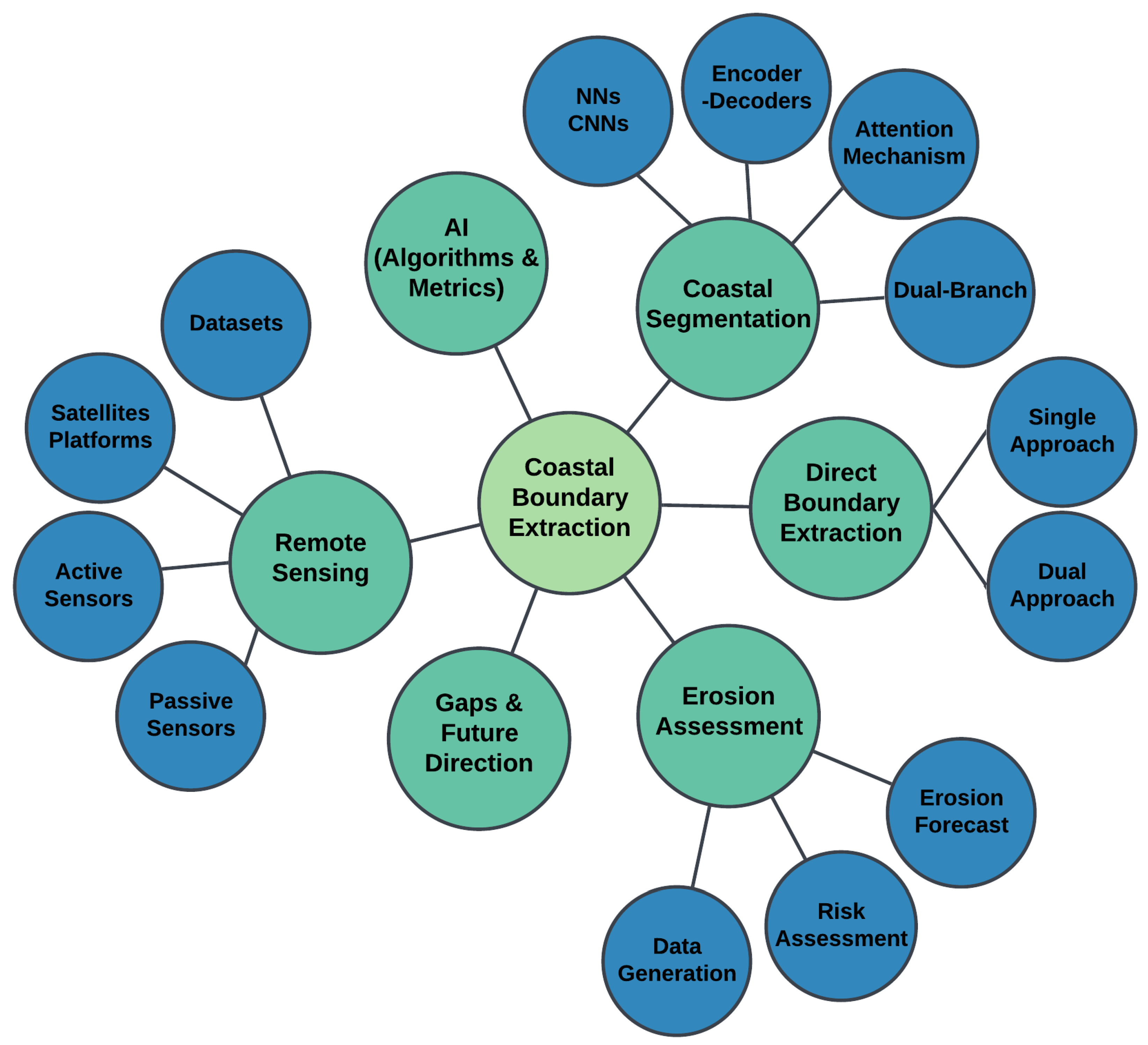
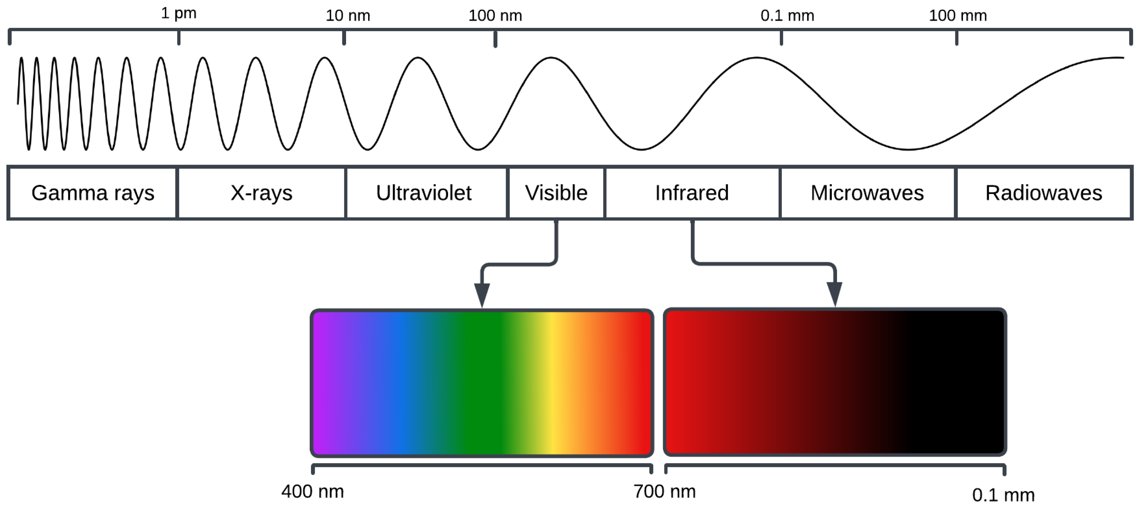
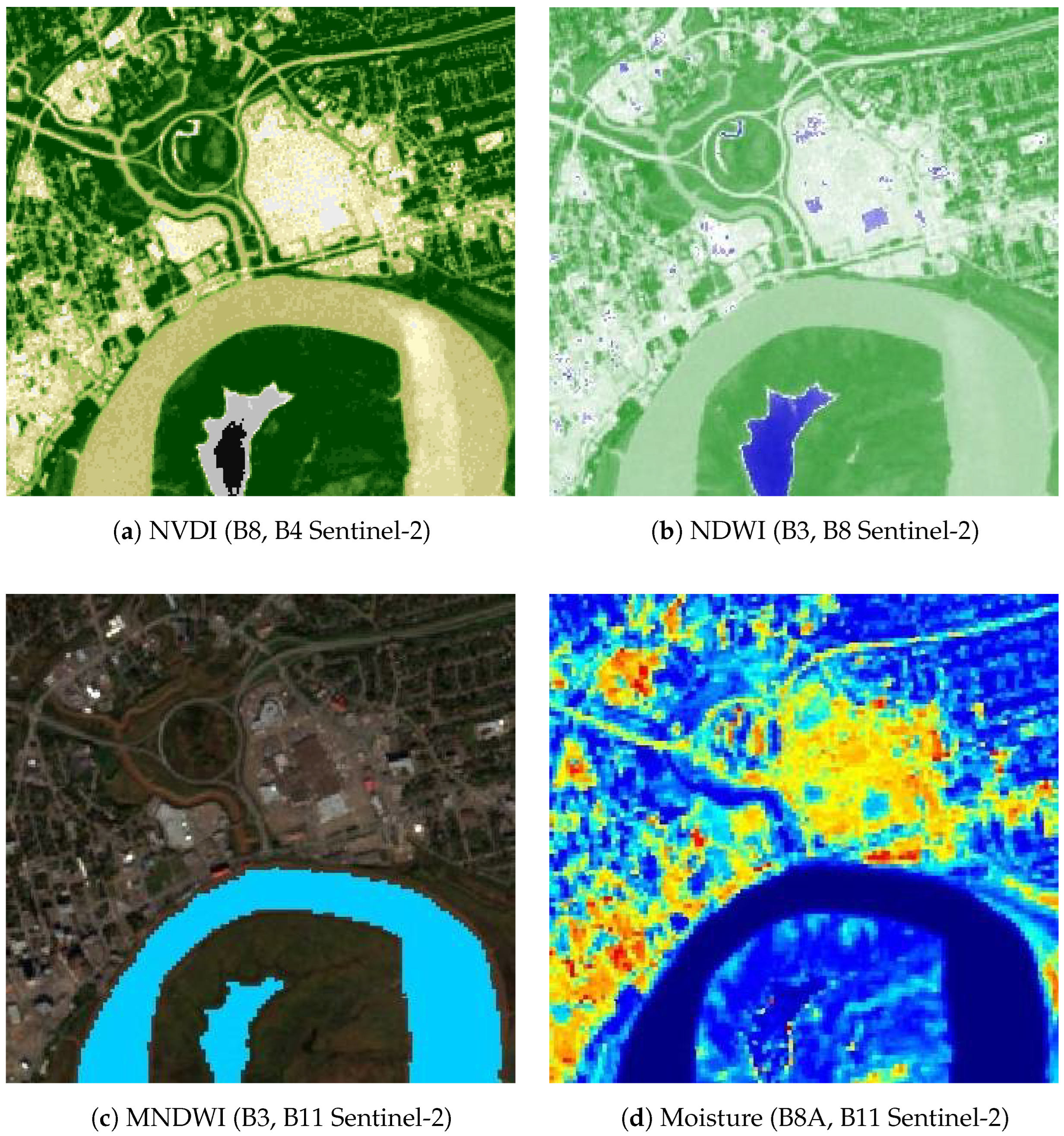
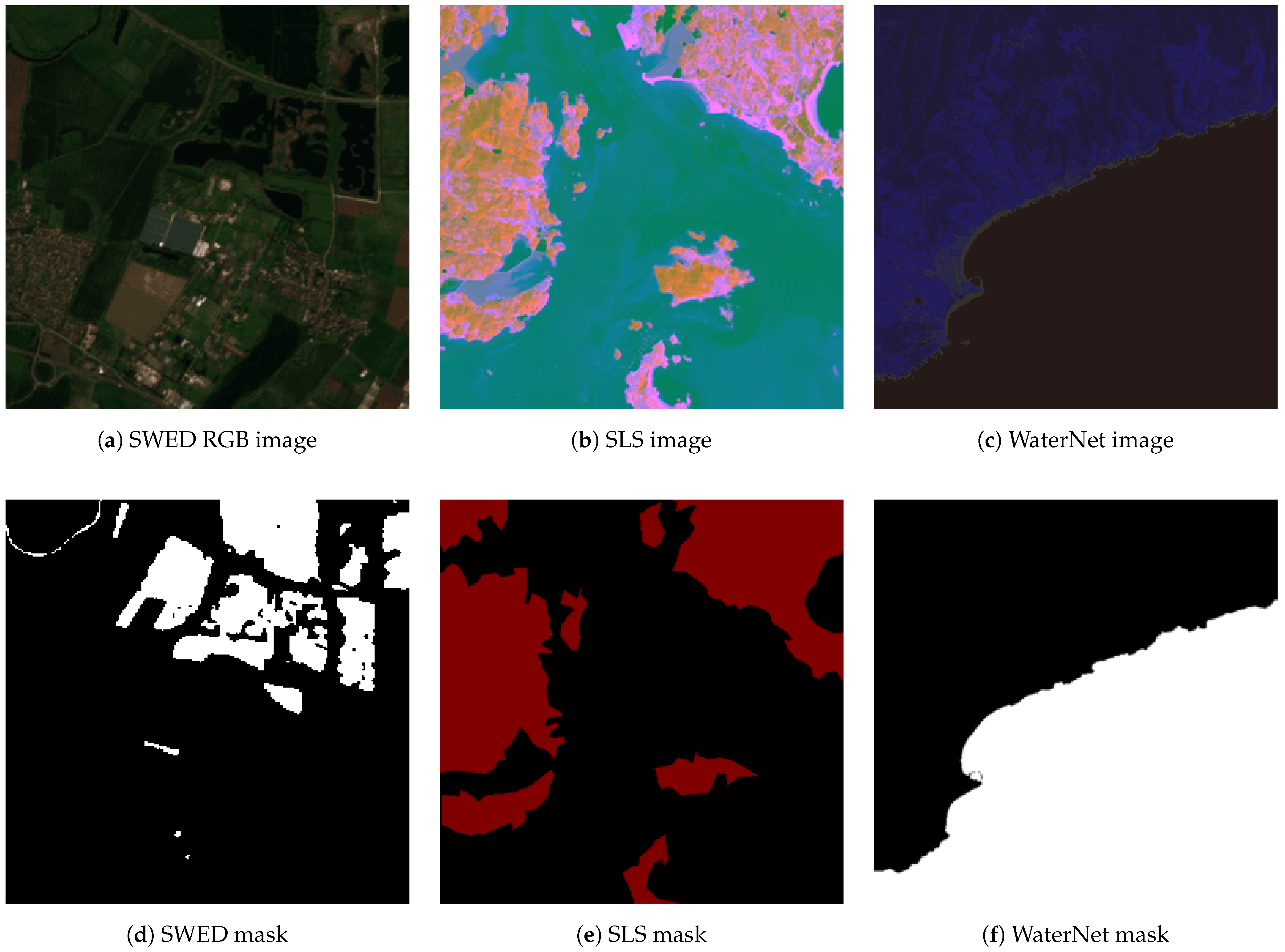
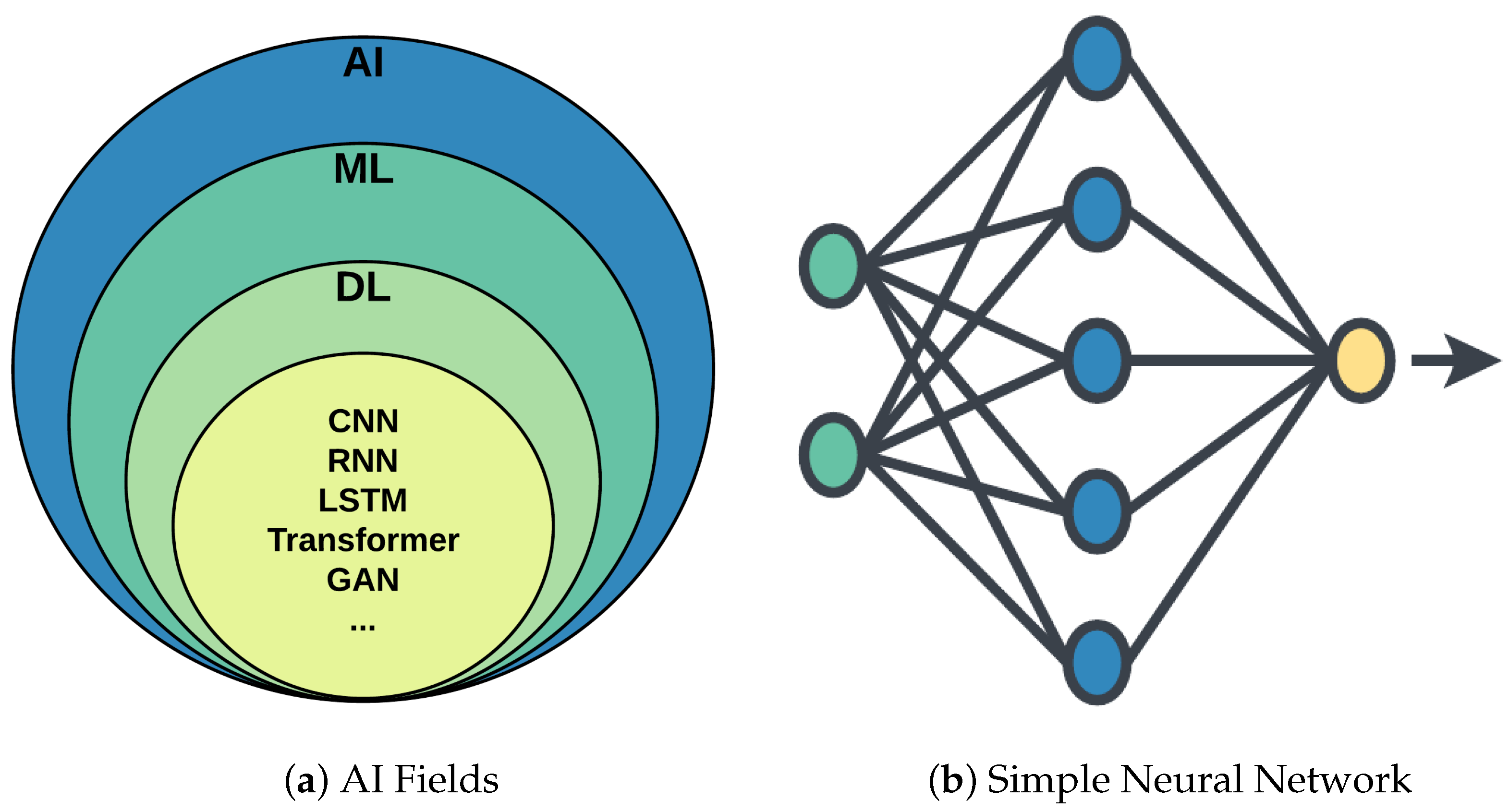
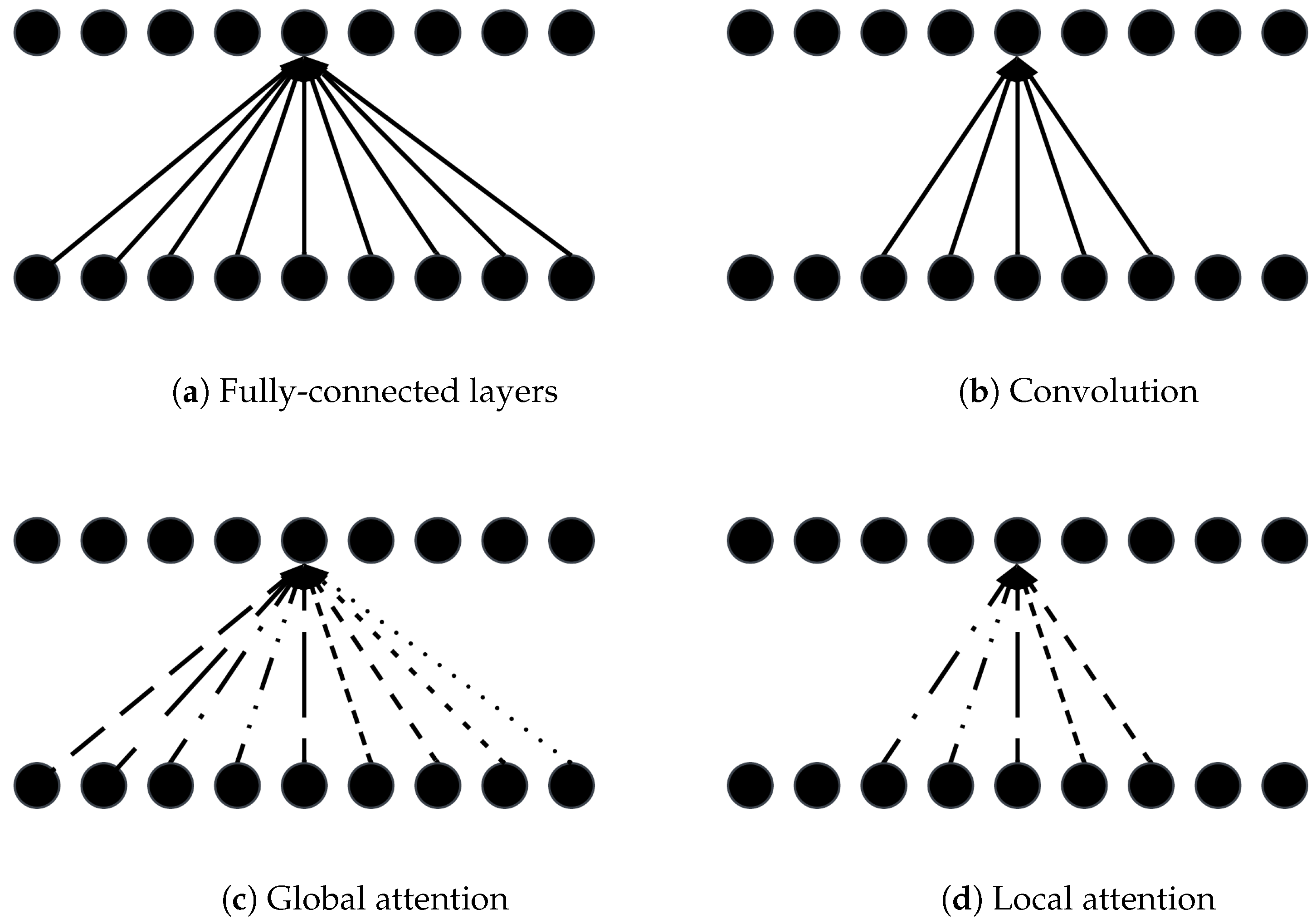
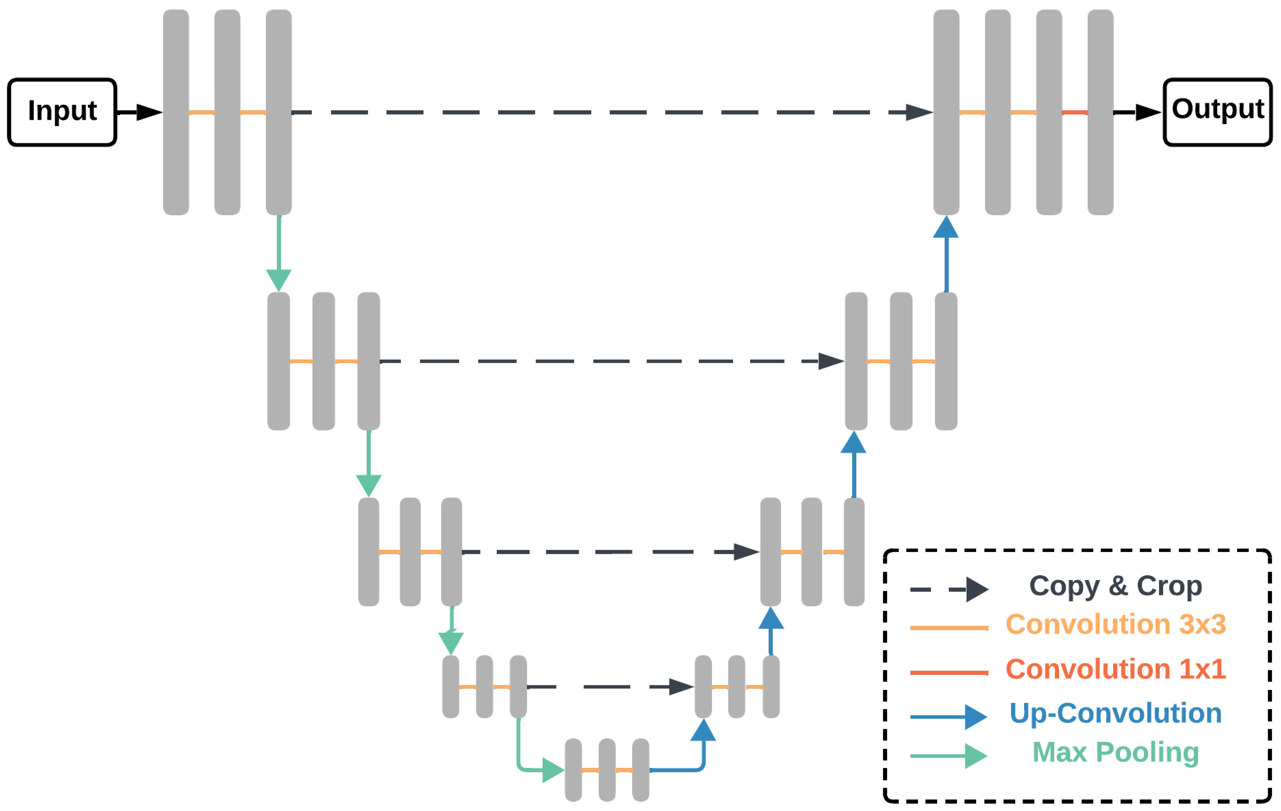
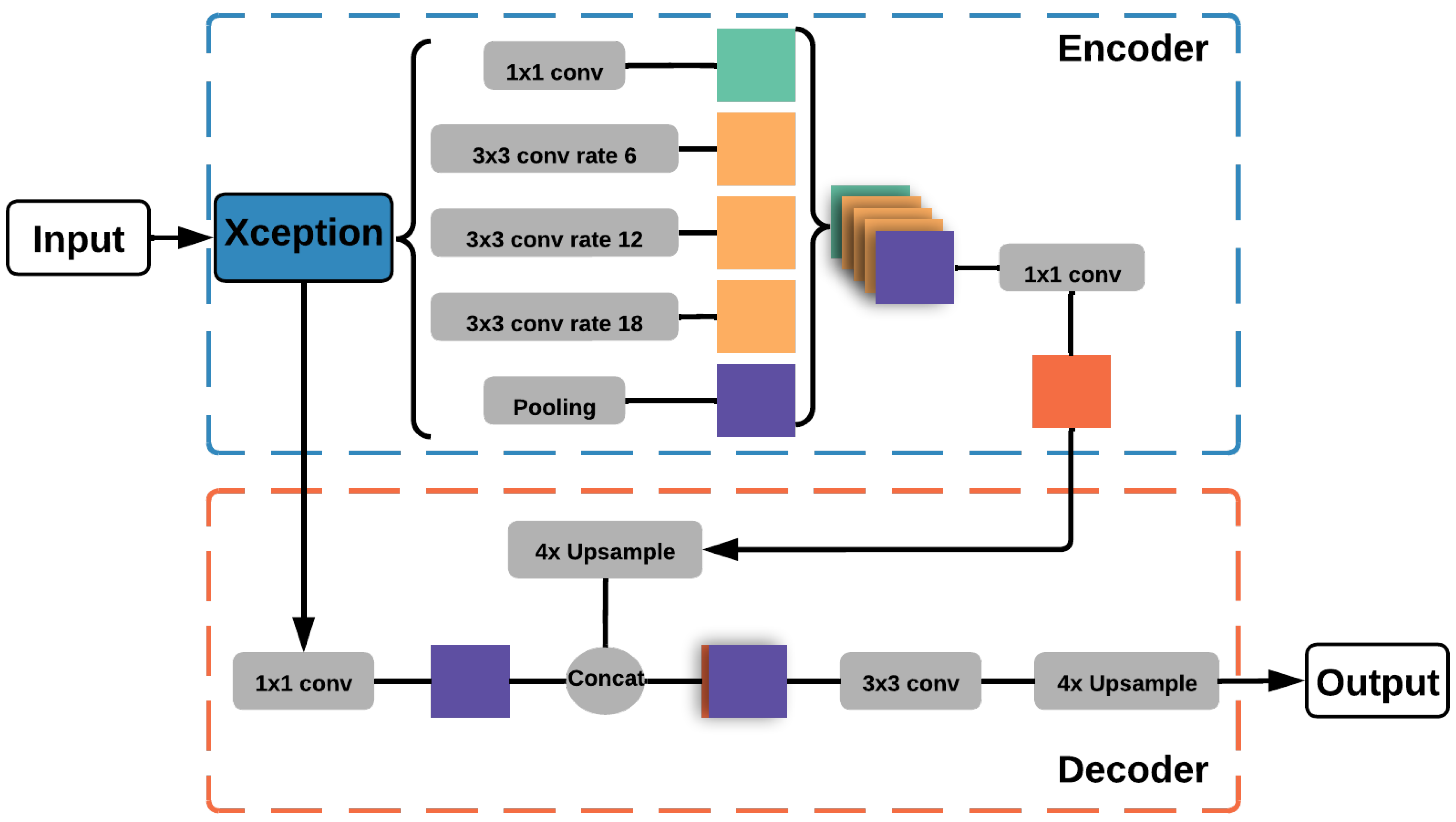
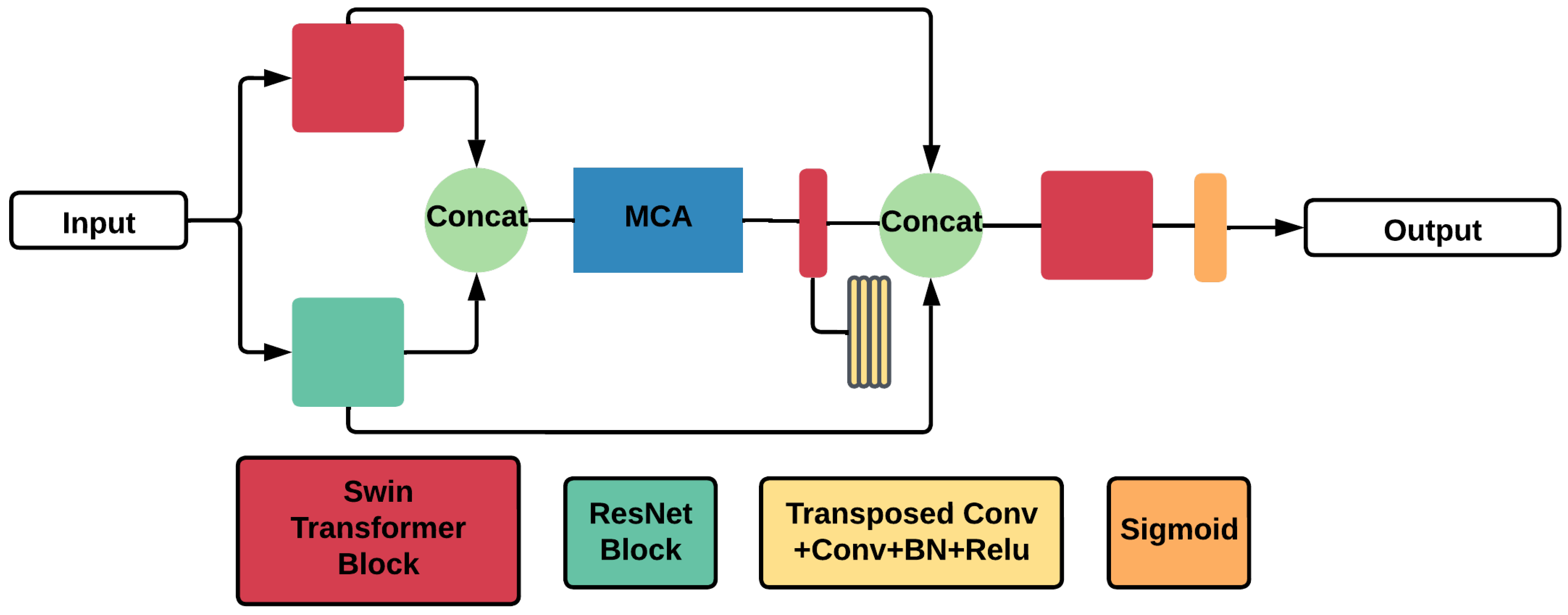
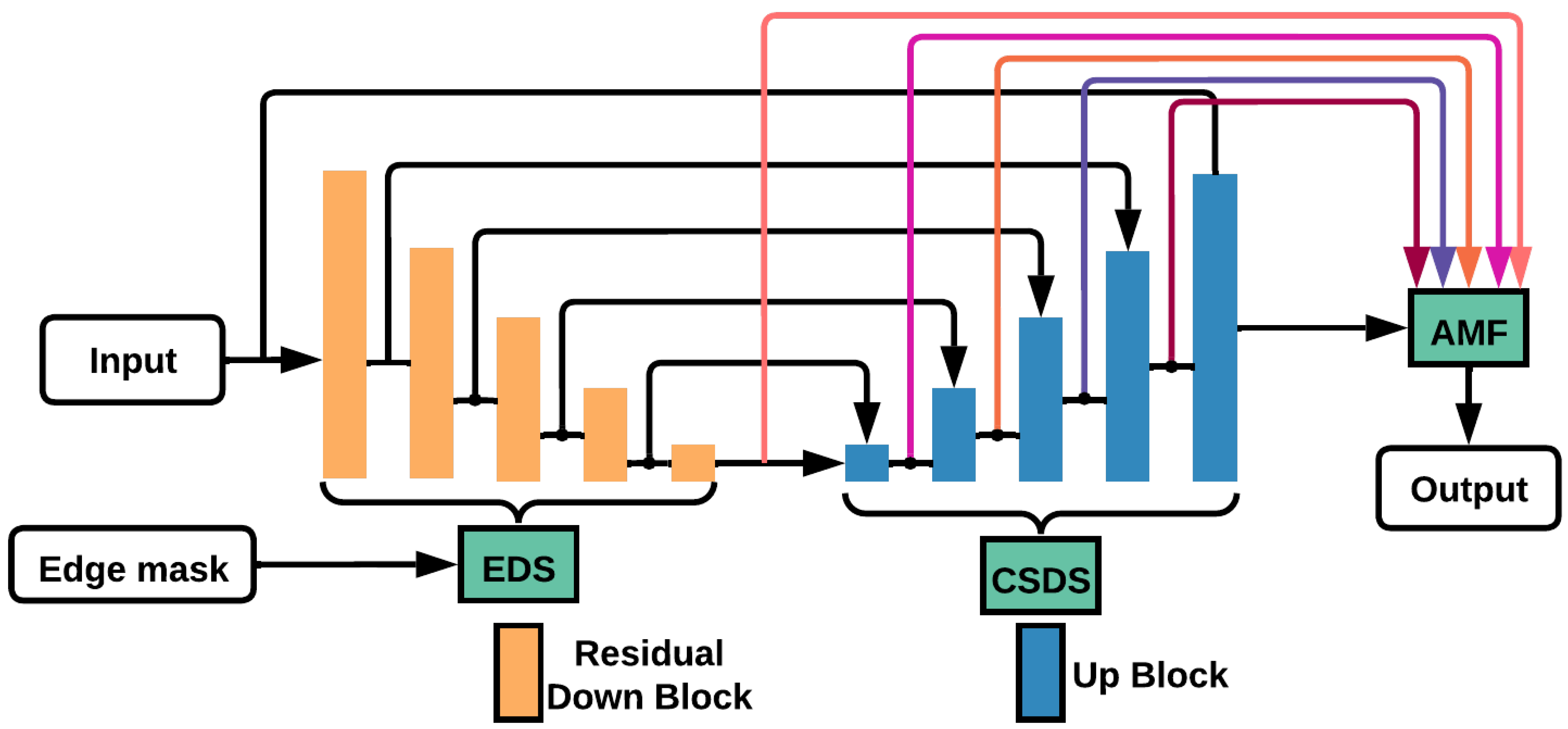
Figure 1. Overview of the review structure.
Geomatics 05 00009 g001
Figure 2. Electromagnetic spectrum.
Geomatics 05 00009 g002
Figure 3. Results of pan-sharpening.
Geomatics 05 00009 g003
Figure 4. Visualization of composites: FC1 (NIR, Red, Green), FC2 (NIR, SWIR2, Red) and true color (Red, Green, Blue).
Geomatics 05 00009 g004
Figure 5. Examples of indices for the same region.
Geomatics 05 00009 g005
Figure 6. Examples of datasets: RGB in the first row, the corresponding masks in the second.
Geomatics 05 00009 g006
Figure 7. (a) AI subsets showing the hierarchy of AI, ML and DL. (b) A simple neural network diagram explaining its components.
Geomatics 05 00009 g007
Figure 8. Differences in algorithms.
Geomatics 05 00009 g008
Figure 9. UNet structure.
Geomatics 05 00009 g009
Figure 10. DeepLabV3+ structure.
Geomatics 05 00009 g010
Figure 11. DANet-SMIW structure.
Geomatics 05 00009 g011
Figure 12. SRMA structure.
Geomatics 05 00009 g012
Figure 13. LaeNet structure.
Geomatics 05 00009 g013
Figure 14. CSAFNet structure.
Geomatics 05 00009 g014
Table 1. Spectral bands and their applications.
BandSpectral Range (nm)Applications and Uses
PAN400–700High spatial resolution monochromatic images; fine details about landscapes and terrain; often used with other bands (pan-sharpening).
Coastal (deep blue)400–450Monitors water quality; detects shallow water features, sediment levels and chlorophyll concentrations.
Blue400–500Monitors water quality and turbidity; detects shallow water features and water bodies.
Green500–600Differentiates land from water; supports plant health and land use mapping.
Yellow580–590Monitors specific crops, algae and water quality.
Red600–700Evaluates vegetation and crop health, soil condition and vegetation indices.
Red edge680–730Tracks plant stress and vegetation health.
Near-infrared (NIR)700–1300Monitors vegetation health, detects water bodies and maps land use and vegetation indices.
Short-wave infrared (SWIR-1)1300–2000Measures soil and vegetation moisture, assesses drought and identifies vegetation stress.
Short-wave infrared (SWIR-2)2000–2500Differentiates minerals, rocks and materials; detects fires; supports geological studies.
Mid-infrared (MWIR)3000–5000Monitors surface temperature, thermal variations and fires; identifies clouds and moisture levels.
Long-wave infrared (LWIR)8000–14,000Provides thermal imaging; monitors surface temperatures, urban heat and climate studies.
Table 2. Specifications of various passive sensor satellites used for remote sensing.
SatelliteBands and ResolutionsRevisit TimeAvailabilityAcquisition Range
Landsat-7PAN (15 m); RGB, NIR, SWIR1, SWIR2 (30 m); Thermal (30 m, resampled from 60 m)16 daysFree on EarthExplorerApril 1999–Present (Extended mission)
Landsat-8PAN (15 m); Coastal, RGB, NIR, SWIR1, SWIR2, Cirrus (30 m); TIRS1, TIRS2 (30 m, resampled from 100 m)16 days, 8 days (w/Landsat-9)Free on EarthExplorerMarch 2013–Present
Landsat-9Same as Landsat-816 days, 8 days (w/Landsat-8)Free on EarthExplorerOctober 2021–Present
Sentinel-2RGB, VNIR (10 m); VNIRs, SWIRs (20 m); Coastal, SWIRs (60 m)10 days, 5 days (constellation)Free on Copernicus HubJune 2015–Present
PRISMAPAN (5 m); VNIR/SWIR (30 m)VariableFree accessMarch 2019–Present
Gaofen-1/6PAN (2 m); RGB, NIR (8 m); WFV (16 m)4 daysCommercial, some research accessJuly 2013–Present (Gaofen-1); June 2018–Present (Gaofen-6)
WorldView-1PAN (0.50 m)1.7 daysCommercial, some research accessSeptember 2007–Present
WorldView-2PAN (0.48 m); Coastal, RGB, Yellow, Red-Edge, NIR1, NIR2 (1.48 m)1.1 daysCommercial, some research accessOctober 2009–Present
WorldView-3PAN (0.31 m); Coastal, RGB, Yellow, Red-Edge, NIR1, NIR2 (1.24 m); SWIR (8 bands at 3.7 m); CAVIS (12 bands at 30 m)<1 dayCommercial, some research accessAugust 2014–Present
WorldView-4PAN (0.31 m); RGB, NIR (1.24 m)<1 dayCommercial, some research accessNovember 2016–January 2019
SPOT-6/7PAN (1.5 m); RGB, NIR (6 m)1–3 days (alone), 1 day (constellation)Commercial, some research accessSeptember 2012–Present (SPOT-6); June 2014–Present (SPOT-7)
PlanetScopeCoastal, RGB, Yellow, Red-Edge, NIR (3–5 m)DailyCommercial, some research access2014–Present
Pleiades-1A/1BPAN (0.50 m); RGB, NIR (2 m)DailyCommercial, some research accessJanuary 2012–Present (Pleiades-1A); December 2012–Present (Pleiades-1B)
Pleiades-NeoPAN (0.30 m); Deep Blue, RGB, Red-Edge, NIR (1.2 m)Twice per dayCommercial, some research accessApril 2021–Present (Pleiades-Neo 3); December 2021–Present (Pleiades-Neo 4)
Terra & Aqua (MODIS)36-band optical-thermal range (2 bands 250 m, 5 bands 500 m, 29 bands 1 km)1–2 daysFree on EarthdataFebruary 2000–Present (Terra); July 2002–Present (Aqua)
Terra (ASTER)Green/Yellow, Red, NIR1, NIR2 (15 m), 6 SWIR bands (30 m), 5 thermal bands (90 m)1–2 daysFree on per requestFebruary 2000–Present
GeoEye-1PAN (0.41 m); RGB, NIR (1.65 m)2–8 daysCommercial, some research accessOctober 2008–Present
Beijing-3NPAN (0.30 m); RGB-NIR (1.20 m)1–5 daysCommercialAugust 2022–Present
Table 3. Specifications of various SAR satellites used for remote sensing.
SatelliteSensorRevisit TimeAvailabilityData Acquisition
Sentinel-1C-SAR: SM (5 m), IWS (5 m × 20 m), EWS (20 m × 40 m), WV (5 m).12 days (single); 6 days (constellation)Free via Copernicus Open Access HubApril 2014–Present
RADARSAT-1C-SAR: single polarization (HH); resolutions: fine (8 m), standard (30 m), ScanSAR (50–100 m).24 daysArchived data on EODMSNovember 1995–March 2013
RADARSAT-2C-SAR: full polarization; resolutions: 1–100 m.24 daysCommercial; some research dataDecember 2007 (Approximate)–Present
RADARSAT ConstellationC-SAR: single, dual, full, compact polarimetry; resolutions: 3 m (spotlight) to 100 m (ScanSAR).12 days (single); 4 days (constellation)Gov/research users onlyJune 2019–Present
Gaofen-3C-SAR: single, dual, full polarization; resolutions: spotlight (1 m), ultrafine (3 m), fine (5 m).29 daysLimited research accessAugust 2016 (Approximate)–Present
SAOCOML-SAR: single, dual, full polarization; SM (10 m), TopSAR narrow (10 m × 50 m), wide (10 m × 100 m).16 days (single); 8 days (constellation)Free via CONAEOctober 2018 (Approximate)–Present
ALOS (PALSAR)L-SAR: single/dual polarization; resolutions: fine (10 m), polarimetric (30 m), ScanSAR (100 m).46 daysArchived data via JAXAJanuary 2006 (Approximate)–12 May 2011
ALOS-2L-SAR: single, dual, full polarization; resolutions: spotlight (3 m × 1 m), ultrafine (3 m), fine (10 m), wide (60 m).14 daysCommercial/research dataJune 2014–Present
TerraSAR-XX-SAR: single polarization; resolutions: spotlight (1 m), SM (3 m), ScanSAR (40 m).11 daysCommercialJune 2007–Present
Capella SpaceX-SAR: single polarization; resolutions: spotlight (0.5 m), SM (3 m), ScanSAR (10 m).Hours (Constellation of 36 satellites)CommercialMarch 2019 (Approximate)–Present
ICEYEX-SAR: single polarization; resolutions: spotlight (0.5 m), strip (1 m), scan (3 m).Max 20 h (Constellation of 38 satellites)Commercial; some free dataJanuary 2018–Present
Table 4. Summary of available coastal datasets.
DatasetSourceResolutionDatesRegionsDescriptionImage–Mask Pairs
Scarpetta et al. [65]Sentinel-2 Level-1C10–60 mDec 2016–2022Hawai’i, NW/NE Continental USA, Great Lakes, Gulf of Mexico, Puerto Rico894 labeled tiles, 13 bands (RGB, NIR, SWIR) excluding Alaska and rivers, derived from NOAA’s CUSP.
SNOWED [66]Sentinel-2 Level-1C10–60 mJun 2015–2023USA coastal regions (Continental USA, Alaska, Hawaii, USA Virgin Islands, Pacific Islands, Puerto Rico)4334 labeled tiles, 13 bands (RGB, NIR, SWIR), derived from NOAA’s CUSP and automated labeling
Seale et al. (SWED) [60]Sentinel-210 m2017–2021Global, various high and low tide regions114 RGB image–mask pairs, 12 interpolated bands, semi-supervised clustering.
Yang et al. (SLS) [62]Landsat-8 OLI30 m2013–2018Chinese coastline1950 training and 1411 test patches, manually segmented using LabelMe.
YTU-WaterNet [64]Landsat-8 OLI10 m2017–2019Albania, Argentina, Bulgaria, England, Georgia, Greece, Ireland, Italy, Libya, Russia, South Africa, Spain, Turkey, USA824 training, 92 validation, 92 test images with segmentation maps from OpenStreetMap.
Coast-Train [67]Aerial, Satellite Images0.05–1 m (aerial), 10–15 m (satellite)2008–2021USA Pacific, Gulf of Mexico, Atlantic, Great Lakes502 training and 34 validation RGB images with detailed masks, up to 12 classes.
Pollard et al. [68]Environment Agency, UK0.10–0.25 m (aerial), 0.25–2 m (LiDAR)2001–2019 (aerial), 1999–2009 (LiDAR)UKHigh-resolution dataset combining aerial photography, LiDAR, field surveys; includes metadata for erosion monitoring.
Global Coastline Explorer [55]USGS30 m2014Global (5 continents, 21,818 large islands, 318,868 small islands)Over 4 million segments classified into 81,000 coastal units with ecological attributes.
GSHHG [57]NOAA, University of Hawai’i200 m–100 kmPre-1996GlobalSix shoreline types, five resolution levels; integrates three data sources (shorelines, lakes, rivers).
Natural Earth Data (NED) [58]Community-maintained10, 30, 100 mUnknownGlobalPhysical and cultural data for cartography and visualization.
OpenStreetMap (OSM) [59]Community-maintainedVaryingOngoingGlobalPolygons separating land and sea, widely accessible for remote sensing.
Table 24. Accuracy of sea–land segmentation using HED-UNet with different loss functions and optimizers.
ModelAdam + BCEAdam + FocalSGD + BCESGD + Focal
Val. Acc. (%)93.397.272.095.6
Test Acc. (%)91.598.359.793.1
Disclaimer/Publisher’s Note: The statements, opinions and data contained in all publications are solely those of the individual author(s) and contributor(s) and not of MDPI and/or the editor(s). MDPI and/or the editor(s) disclaim responsibility for any injury to people or property resulting from any ideas, methods, instructions or products referred to in the content.

